
Lesson Files | Lessons > Lesson_13 > 13_Starter Budget.xls Lessons > Lesson_13 > 13_Budget_End.numbers Lessons > Lesson_13 > 13_Draft.png |
Time | This lesson takes approximately 60 minutes to complete. |
Goals | Create a basic to-do checklist and a travel budget Work with templates in Numbers Understand key spreadsheet terms Convert a Microsoft Excel file into a Numbers spreadsheet Add header rows, header columns, and footer rows Format cell contents Format a table using styles Use formulas and functions to calculate cell values Add and resize a graphic object Size and print a spreadsheet Save a spreadsheet as a PDF or an Excel file |
Numbers is an easy-to-use spreadsheet program with a flexible, free-form canvas that you can use to organize data, manage lists, create tables and charts, insert graphics, and place text anywhere on the page. The program supports over 250 math functions that perform complex calculations with just a few mouse clicks.
If you’ve used other spreadsheet programs, such as AppleWorks or Microsoft Excel, Numbers will seem familiar from the moment you open it. The good news is, Numbers offers some innovative features that let you create great-looking spreadsheets with less work—features like intelligent tables, customizable checkboxes and sliders, 2D and 3D charts, and ready-made templates for home, education, and business uses.
In this lesson, you’ll use Numbers to create a simple to-do checklist and a travel budget. Along the way, you’ll learn spreadsheet essentials—the basics of working with data tables and calculations—as well as how to use templates and how to import, enhance, and export Microsoft Excel spreadsheets.
We’ll start by opening a blank Numbers spreadsheet. After exploring the Numbers interface, we’ll create a to-do checklist and use the inspectors and format bar to make adjustments to the rows, columns, and cells. Next, we’ll create a basic business travel budget and use the tools in Numbers to calculate expenses. We’ll also format the report to present the data in a clear and accurate way that helps make it more readable. Finally, we’ll save the completed budget as both Numbers- and Excel-compatible spreadsheets that you can share on the Internet.
You can open Numbers in three ways:
In your Applications folder, open the iWork ’09 folder and double-click the Numbers icon.
In the Dock, click the Numbers icon.
Double-click any Numbers document.
For this exercise, you’ll open Numbers using the first method.

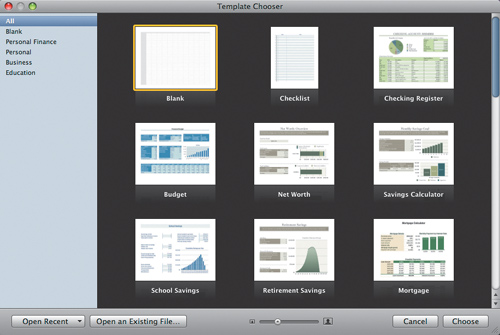
When you first open Numbers, you’ll see the Template Chooser, which lets you choose Apple-designed templates (along with any custom templates you’ve created and saved).
Choose File > New from Template Chooser to open the Template Chooser.
Templates are the quickest way to begin a project, because much of the formatting has already been done for you. They’re great starting points, with ready-made data, formulas, charts, and formatting that can save you loads of time and make data calculation easier (and even fun). You can edit templates to suit your content, modifying everything from font style and color to chart types and formulas.
Take a moment to browse through the various templates for home, work, and school by clicking each of the five categories. This will also give you a visual overview of some of the capabilities of Numbers.
Move the pointer over a thumbnail to preview each template.
Drag the resize slider at the bottom of the Template Chooser to see larger thumbnails.
Click the Open Recent button at the bottom of the Template Chooser to access recently opened documents with a single click.
Now let’s open a blank template and get started on a basic spreadsheet with a to-do checklist.
In the Template Chooser, click to select the Blank category, and then select the Blank template.
Click Choose to open a new document based on the Blank template.
Choosing the Right Template for the Job
The Template Chooser in Numbers is organized into five categories that make it easier to find the right template for your needs. Here’s a quick guide to some particularly useful and well-designed templates in Numbers.
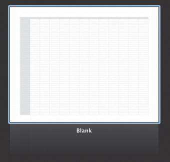
Only two templates are in this category, but both are useful. Blank is a standard spreadsheet with no formatting. Use it when you want to build your spreadsheet from scratch. Checklist is a good starting point for creating to-do lists, packing lists, order forms, or any other list-based data. These are the basic starting points for all custom spreadsheets.
</division>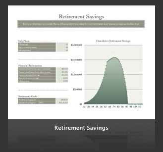
This category contains some great tools that can help you manage individual or household finances. Look here for financial management templates such as Budget, Checking Register, Mortgage, and Savings Calculator, as well as financial planning templates such as School Savings and Retirement Savings.
</division>
This category contains some beautiful project-planning forms for uses ranging from special events and dinner parties to garden and home improvement. Thanks to their rich graphics, these templates are great for personal and home improvement and offer easy starting points for organizing your life in an attractive way that can be easily shared. In particular check out Dinner Party, Home Improvement, and Travel Planner.
</division>
Designed primarily for small businesses, this category includes some great templates for standard business needs, like invoices and expense reports, along with some more complex financial analysis templates. Don’t miss Invoice, which helps you bill clients in a professional manner, and Financials, for analyzing your company’s performance.
</division>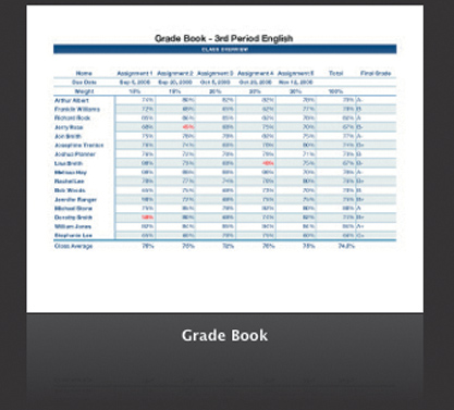
The Education category brings organization to the classroom. It includes two useful projects for elementary and high school science labs, which help students document their research with both data and graphics. Teachers will also find templates for generating grade books and math quizzes.
You can find even more templates created by the Apple community by visiting iWorkCommunity.com Template Exchange (www.iworkcommunity.com) and Numbers Templates (www.numberstemplates.com).
</division>Now let’s get to work on our starter spreadsheet and learn the basics of managing sheets, entering data, and formatting cells to best display the information. The first step is to understand how Numbers organizes information.
Each Numbers spreadsheet includes one or more sheets. Think of sheets as tabs or subdivisions within your document. Typically, sheets are used to organize the spreadsheet information into smaller, more manageable groups. For example, you might put all your raw data and assumptions on one sheet and, on a second sheet, present your final conclusions and charts.
Our blank spreadsheet opens with only one sheet. You can see a list of all the sheets in the document in the Sheets pane, located above the Styles pane in the upper left corner of the canvas. In this exercise, we’ll experiment with naming, adding, deleting, and reordering sheets.

To rename the sheet, double-click its name (currently Sheet 1).
Enter a new name that better describes what the sheet is about. For this example, type Expense Report, and press Return.
Let’s add a second sheet to the document.
To add a new sheet, click the Sheet button in the toolbar (or choose Insert > Sheet).
A second sheet, called Sheet 2, is added to the document. Notice that Numbers also added a second table on the new sheet. You’ll look at tables in the next section.
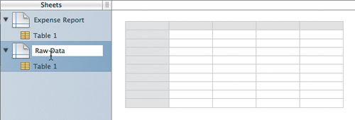
Rename the new sheet Raw Data.

You can reorder your sheets to change how the data is presented for printing or viewing.
In the Sheets pane, click to select the Raw Data sheet; then drag it to the top of the Sheets pane to make it first in the list.
As you add sheets in a document, the Sheets pane can become crowded; it’s sometimes useful to view just the sheets without their contents listed.
Hide the contents of both sheets by clicking the disclosure triangles to the left of each sheet’s name.
Tip
If you are using a laptop with Multi-Touch trackpad support, you can navigate between sheets with the three-finger swipe gesture (place three fingers on the trackpad and drag up or down).
That’s all it takes to manage sheets in your document. Being able to rename and reorder sheets is important as your spreadsheets grow in complexity. Next, let’s explore a table.
Within a single sheet you can have one or more tables. Tables are simple grids, with horizontal columns and vertical rows, used to organize, analyze, and present data.
Typically, when you build a spreadsheet, you spend most of your time working with tables. A unique feature in Numbers is the ability to use multiple tables and, on a single sheet, mix them with other media such as charts or graphics. Numbers lets you build and format tables in numerous ways, and lets you handle different types of data intelligently within your tables. You can sort, sift, categorize, and conditionally format your data quickly and easily.
Note
Many of the templates include preformatted tables that make it faster to set up tables with your own data and images.
Let’s take a moment to learn the “language” of tables. In this exercise, you’ll practice with Numbers using a blank spreadsheet. Later in the lesson, you’ll create a useful to-do checklist.
Click the middle of the Raw Data sheet on your canvas to select it.

Notice that numbers and letters appear at the edges of the table. These reference tabs help you identify and navigate the contents of your spreadsheet.
By clicking in the sheet, you have selected a cell A cell is an individual box within a table that can contain data.
Look across the top of the active sheet and click the letter C.
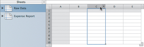
By clicking a letter, you have selected a column. Columns are a vertical array of cells that is one cell wide. Each column uses a letter in the reference tab for identification.
Look down the left edge of the active sheet and click the number 7.

By clicking a number, you have selected a row. Rows are a horizontal array of cells that is one cell tall. Each row is labeled with a consecutive number in the reference tab on the left edge of the table.
Now that you know how to identify individual rows and columns, let’s select a specific cell. A cell is identified by the intersection of its row and column.
Select cell B8.

This cell is located at the intersection of column B and row 8.
All sorts of tables are available to choose from in Numbers, so now let’s experiment with adding two specific kinds of tables to the spreadsheet: Basic and Checklist.
Click the disclosure triangle next to the Raw Data sheet to see all of its tables.
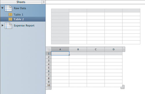
In the toolbar, click the Tables button and choose Basic from the pop-up menu.
Another table (called Table 2) is added to the sheet. This table is smaller than Table 1, but like all tables, it can be resized or repositioned to meet your needs.
You can also add tables using a menu command. Let’s create a to-do list by adding a Checklist table.
Choose Insert > Table > Checklist. Table 3 is added to the sheet.
Next, let’s add some text.
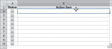
Click in cell A1 and type Status. Press Tab to switch to the next cell.
In cell B1, type Action Item, and press Return.
The table is looking clearer. But a to-do list should have some dates to help organize the information. Let’s add one more column to hold the date information.
In Table 3, the checklist table, click column B to select it.
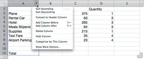
Click the reference tab pop-up on the upper right corner of column B and choose Add Column Before.
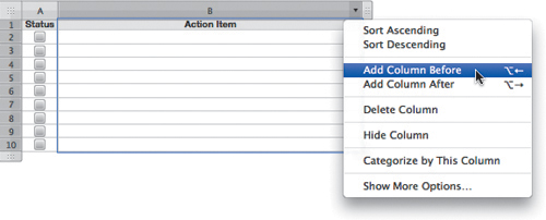
A third column is added to the sheet.
Label the newly created column B as Due Date.
To enter a date in the new column B, click in cell B2 and type 12/15/09. Press Return.

Numbers interprets the data as a date and displays Dec 15, 2009. This is the default format for displaying a date, but let’s say you want a different format for the dates in this checklist.
Click column B to select all the cells. By selecting the entire column, you can reformat all the cells to match.
In the format bar at the top of your screen, click the Cell Format pop-up menu. Choose Date & Time, and then choose from the list the display format that shows the full month, date, and year.
The date will be reformatted in the selected column.

Note
The date in the format menu will be based upon the current date and time. Your menu may look slightly different.
Next, let’s resize the date column so that it takes up less room in the table.
Place the pointer between columns B and C in the table until it changes to a double arrow.
Drag to the left to make column B narrower.

A width of 2.00 in allows plenty of room for the date but avoids wasted space.
Choose File > Close to close this practice spreadsheet.
Save the starter spreadsheet only if you want to use it to practice more on your own.
Now that you know how to work with sheets, tables, rows, and columns, you can say good-bye to your starter spreadsheet and move on to the fun stuff: formulas, functions, and more sophisticated formatting of complex documents.
In this exercise, we’ll create and work with a business travel budget. To save you from having to type in the data, we’ll start by importing a basic spreadsheet that already has the data entered. We’ll then use Numbers to make the report more attractive, more readable, and more functional.
And to make it more interesting, the spreadsheet we’ll import is a Microsoft Excel document. If you’ve worked with spreadsheets before, you’ve probably used an Excel workbook, a common format. Numbers has excellent support for opening, working with, changing, and saving Excel files, so it’s easy to share documents with Microsoft Office users.
Note
Numbers can import data from several other common formats, including files saved in comma-separated value (CSV) format, tab-delimited format, Open Financial Exchange (OFX) format, and AppleWorks 6. Numbers supports Microsoft Excel 2008 and earlier formats for both Mac and PC.
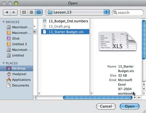
Choose File > Open and navigate to the Lesson_13 folder.
Choose 13_Starter Budget.xls and click Open.
Numbers opens the Excel spreadsheet and imports it to a Numbers file. The new Numbers document has three sheets, each with a table. However, the second two sheets are blank, so let’s go ahead and delete them now.
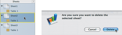
Select Sheet 2 and click Delete. Numbers asks you to confirm that you want to delete the selected sheet. Click Delete.
Choose File > Save.
In the Save As field, name the file 13_Starter Budget.numbers.
If your file folder isn’t visible in the Where pop-up menu, click the disclosure triangle to the right of the Save As field.
Specify a location (such as the chapter folder) in which to store the file.
Click Save to save the file to your hard drive.
When you save a Numbers spreadsheet, all of the graphics and formatting are stored within the document so that it can be easily transferred to another computer.
Now that the data is imported to your spreadsheet, let’s format the table to help us calculate and analyze the data.
To improve the readability of your tables, you can use formatting tools to stylize the cells and layout. Although you may think this is done only for aesthetic reasons, remember that in most instances, it’s important to make your information easy to read. There are three primary ways to access formatting tools:
By using a header row and column, you can add a label that describes the contents of a table’s rows and columns. Header rows and columns are usually formatted so that they stand out. A footer row can also call out data that has been totaled.
A header row uses the topmost cell of each column.
A header column is the leftmost column in the table.
Note
A major benefit of using header rows and columns is that they appear on each page when you print a table. This information ensures that your data is clearly labeled and makes the table easier to read.
In this exercise, you’ll add a header row, header column, and footer row to your table:
In the canvas, select the table by clicking it.
You will know a table is selected when the column and row labels appear.
Click the reference tab for column A to select the leftmost column.
Position your pointer over the reference tab of column A to display its disclosure triangle. Click the triangle, and from the pop-up menu, choose Convert to Header Column.
Click the reference tab for row 1 to select the topmost row.
Pause your pointer over the reference tab of row 1 to display its disclosure triangle. Click the triangle, and from the pop-up menu, choose Convert to Header Row.

The table is already much easier to read because the information has been visually organized. Now you’ll add a footer row to draw attention to the bottom row of the table. By formatting the Total row, you’ll make your totals stand out more clearly.
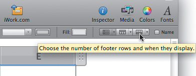
With the table selected, click the Footer button in the format bar to add one. A new footer is added to the bottom of the table.
Click cell A11 to select it.
Choose Edit > Cut to move the selected text to the Clipboard.
Click cell A12 to select it.
Choose Edit > Paste and Match Style to write the text to the new cell but retain the formatting of the target cell.
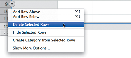
Drag across rows 9, 10, and 11 to select them.
Pause your pointer over row 9. When the disclosure triangle appears, click it, and from the pop-up menu, choose Delete Selected Rows.
Press Command-S to save the changes to your document.
By formatting cells in a table, you display data in specific ways. For example, in this table, you can designate data in the Cost column as monetary values and display those values with a currency symbol (such as $, £, or ¥).
Note
When formatting cells, you are only setting the display characteristics of the cells (not changing their data). When a cell is used in a formula, its actual value is used.
There are two easy ways to define cell formats:
Use the format bar to access the most common controls.
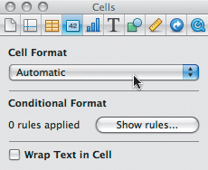
Use the Cell Format pop-up menu in the Cells inspector.
Note
Even empty cells can be formatted. When you add text to a formatted cell, it displays according to the cell’s formatting. Deleting text from a formatted cell removes that value from the cell but retains the cell formatting.
Click the reference tab for column C to select the column.
In the toolbar, click the Currency Format button.
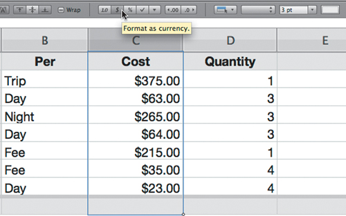
The cells with number values now have $ symbols and display two decimal places, which is standard with this type of currency.
Click the reference tab for column E to select it.
This column will be used as a subtotal column.
In the toolbar, click the Currency Format button.
Click cell E1 and type Subtotal to label the cell.
The data is formatted correctly but it’s not as easy to read as it might be. To improve the readability, you’ll now center some of the data in the cells.
Click the reference tab for row 1 to select all of the column labels in the header row.
In the format bar, click the Center Alignment button to center the labels on these columns.
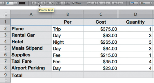
Choose Edit > Select All to select the entire table. Then, in the format bar, click the “Align text to the bottom of a table cell, text box, or shape” button to align the text labels to the bottom of the rows.

Click the reference tab for column B to select the column.
Command-click column D to add it to the selection. Pressing the Command key while clicking lets you select multiple items that are not adjacent.
In the format bar, click the Center Alignment button to center the text in these columns.

Press Command-S to save your travel budget.
Numbers offers powerful and flexible table styles to quickly change a table to a predefined visual format. By applying styles, you can ensure that tables are formatted consistently across your document. Numbers includes several default styles, but you can also create and save your own custom styles.
A table style can define the following attributes:
The table’s background (including color or image) and its opacity
The stroke, color, and opacity of a body cell’s outside border
The outside borders of the header row, header column, and footer row
The background (color or image and opacity) of table cells
The text attributes of table cells
In this exercise, you’ll apply and modify a table style to suit your travel budget.
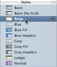
On the canvas, select the current table.
In the Styles pane, click Beige; then try the various styles to see how the table changes as they are applied.
Note
Because you previously formatted cells in the table, those cells retain their formatting. Changes made to an individual part of a table are called overrides. Applying a table style respects these overrides. To clear overrides, place your pointer near the style’s name; then click the arrow to the right of the style you want to apply and choose Clear and Apply Style. For this exercise, you’ll leave the overrides in place.
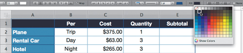
Choose the Blue Headers style to apply it to the table.
Click the reference tab for row 1 to select it.
In the format bar, click the Fill button and choose a dark blue fill color.
Some of the text is being clipped because the cells aren’t big enough. Numbers can fix this problem quickly.
Click a cell in row 9 where the text is clipped. Open the Table inspector and click the Fit Row Height button to automatically adjust the height of the table’s cells to fit the new style.
Now that you’ve created a new table style, you can save it for later use.
Choose Edit > Select All.
With the table selected, move the pointer over any existing style in the Styles pane. Click the arrow to the right of any style and choose Create New Style.
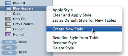
Name the style Blue Two Tone and click OK.
The style is added to the Styles pane of the document. You can easily reuse it on any future tables that you add to this document.
Note
Custom table styles are stored only with the document in which they were created. To store a style for use in other documents, you must create a template from your document. To do so, choose File > Save As Template. Do not save this report as a template because you are not yet finished formatting it with formulas and functions.
Press Command-S to save the changes to your document.
Now that the table is formatted, you can finish it by using formulas to apply mathematical functions to the cell data.
When you use formulas to calculate values based on your table data, you unleash the true power of Numbers. When you enter a formula into an empty table cell, it will display a new (and constantly updated) value in the cell that’s the solution to that formula. In your example spreadsheet, formulas can be used to calculate a budget estimate.
Numbers has several tools for working with formulas and functions:
The Formula Editor lets you create and modify formulas in the spreadsheet. To open the Formula Editor, select a table cell and press the = (equal sign) key.

The formula bar is always visible beneath the format bar and can be used to create and modify formulas.
You can also apply a function, which is a predefined operation that has a name (such as SUM, AVERAGE, or MEDIAN). Functions can be accessed using the Function Browser, or you can find the most common functions already calculated for you beneath the Styles pane.
Now you’ll create some formulas to fill the Subtotal column in your travel budget:
In the canvas, select the table by clicking it.
Click cell E2 to make it active.
Press the = (equal sign) key to open the Formula Editor.
You will create a formula to multiply the cost of each item by its quantity and calculate a subtotal cost for each item.
Click cell D2.
You’ll notice that the formula reads Quantity Plane. The Formula Editor uses the labels from your headers to make formula editing much easier.
Press the * (asterisk) key to indicate that these values will be multiplied.
+ Plus
- Minus
* Multiply
/ Divide
Click cell C2.
Numbers inserts the text Cost Plane into the formula. The formula now reads = Quantity Plane * Cost Plane.
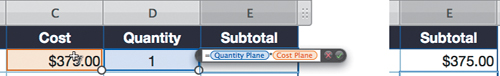
Press Return to apply the formula.
Numbers calculates the correct value of $375.
You can also write formulas in Numbers using only the keyboard, without a mouse or trackpad. Let’s give it a try.
Click cell E3. Press the = (equals) key to open the Formula Editor.
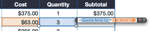
Hold down the Option key while in the Formula Editor to reference cells with arrow keys. Press the Left Arrow to select the adjacent cell.
Press the * (asterisk) key to add a multiply calculation.
Hold down the Option key and press the Left Arrow key twice to select the next adjacent cell.
The formula now reads Quantity of Rental Car * Cost of Rental Car.
Press Return to apply the formula.
You can reuse this formula on similar cells in the spreadsheet.
Click cell E3.
Place your pointer over the fill handle in the lower right corner of cell E3.
The pointer changes to a crosshair.

Drag the fill handle downward to apply the formula to other cells in the column. Drag through cell E8 to apply the formula to calculate all subtotal values in column E.
Now that accurate subtotals exist, we can add all of the subtotals together to create a total budget number. Let’s use a function.
Drag through cells E2 to E8 to select them. These are the numbers you’ll want to add.
From the area below the Styles pane, drag the SUM function to cell E9.
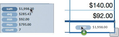
Numbers calculates a correct value of $1,998.00 for the budget estimate. Now you can review your calculations for accuracy.
In the toolbar, click the Formula List button to view a complete list of every formula in your spreadsheet.

Look at each formula to ensure accuracy.
You should see that the Quantity and Cost values are matched (that is to say, Quantity of Hotel * Cost of Hotel).
In the toolbar, click the Formula List button hide the list of formulas.
Press Command-S to save the changes to your document.
Although Numbers is a spreadsheet application, it offers the same robust graphics capabilities as Keynote and Pages. The Numbers document is a free-form graphics canvas that provides great flexibility in arranging your information and graphics on the page:
You’ll find useful layout and graphics tools, including alignment guides; rulers; and Instant Alpha, masking, and drawing tools. These features are explored in the Keynote and Pages lessons of this book, as well as in the online help.
You can add floating text boxes by clicking the Text Box button in the toolbar. These boxes can contain any text and be positioned anywhere on the canvas.
You can add preset shapes or draw your own custom shapes in the spreadsheet.
The iLife Media Browser lets you access photos, movies, and sounds stored on your hard drive, and drag them directly into your Numbers canvas.
Thanks to Numbers’ free-form canvas, you have great visual control over your spreadsheet. To make use of it, let’s add a graphic element and position it on the page:
In the Sheets pane, choose the sheet by clicking its name.
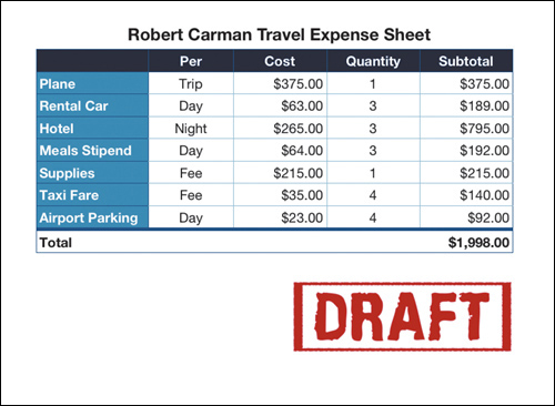
Choose Insert > Choose to choose a file to insert into the sheet.
Navigate to the Lesson_13 folder that you copied to your computer. Choose the file 13_Draft.png and click Insert.
The graphic is added to the page, but it’s a little large, so let’s scale it down.
Click the image to select it. Then drag its selection handle until the image is about 3.5 inches wide. (You can see the width and height displayed next to the image as you drag.)

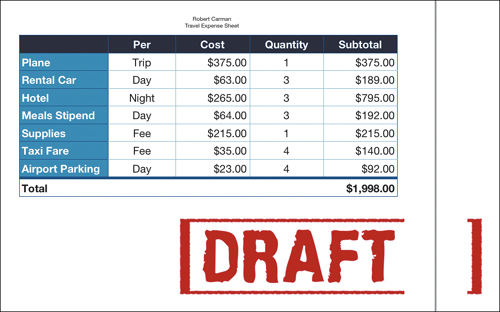
Position the image on the page using the figure for guidance.

The blue alignment guides are useful for positioning the graphic on the page. You’ll make minor adjustments to the image size and position in the next section.
Press Command-S to save the changes to your spreadsheet.
A unique feature of Numbers is its interactive Print View, which makes it easy to prepare your spreadsheet for printing or sharing. Whenever you want to print a sheet or make a PDF for online review, you can use Print View to check the layout.
In the Sheets pane, choose the sheet you’d like to print.
In the toolbar, click the View button and choose Show Print View.
Notice that the page icon at the bottom of the document window is selected. You can toggle Print View on and off by clicking this button.
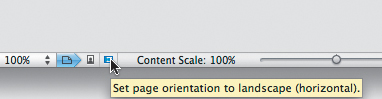
Next to the Print View button you’ll find two buttons for page orientation. Currently, this document is set to portrait (vertical) orientation. Because this table is wider than it is tall, you should switch to Landscape orientation.
Click the Landscape (horizontal) button to change the page layout.
Now that the page is properly oriented, you’ll notice that it doesn’t fill the page as well as it could. Let’s resize the content to get as large a printout as possible.
Drag the Content Scale slider to the right until its value is 175%.
This sizes the table as large as possible while still fitting it all onto one page. You’ll notice, however, that the spreadsheet will print to as many as four pages because the red DRAFT graphic still is wrapping to other pages.
Click the DRAFT graphic and size it by dragging its selection handles.
A new width of about 2.5 inches will work well.
Reposition the graphic by dragging it so that it doesn’t wrap to any additional pages.

Because you are in Print View, elements such as the page header are visible. The current text appears a bit small and could be better formatted for readability.
Click in the header to edit the text.
Delete the hard return between the two lines of text so that the page title appears on one line. Click at the start of the text Travel Expense Sheet and press Delete to remove the gap.
Let’s add a single space between the words Carman and Travel.
Drag though the text to select it.
In the format bar, change the header text to Helvetica Neue Bold at 24-point size, as in the following figure.

Press Command-S to save the changes to your document.
Now that you’ve completed the spreadsheet and set the optimum print size, you can print the document.
When you are ready to print, choose File > Print.
From the Printer pop-up menu, choose the printer you’d like to use.

If the full print window is not visible, click the disclosure triangle next to the Printer field.
In the Copies field, type the number of copies you want to print.
Note
In the print window, you can choose to print all sheets or just the current sheet. This makes it easy to print only the pages you want. Additionally, you can select the “Include a list of all formulas in the document” checkbox to print additional pages that will show all of the calculations performed.
Click Print.
Because spreadsheets are generally used collaboratively, it’s useful to be able to export your Numbers spreadsheet to a variety of formats. Numbers files can also be easily emailed or posted to iWork.com for sharing over the Internet.
The Portable Document Format (PDF) is an industry-standard format that can be viewed using applications such as Preview on a Mac or Adobe Reader on a Mac or PC.
PDF files are compatible with most computer platforms and are an easy file format to use for document sharing. Many portable devices, such as handheld computers and iPhones, can display PDF files. You can also password-protect a PDF file against editing, which makes it a good choice when you want to retain a document, such as a budget, in its original form.
Choose Share > Export to open the Export controls.
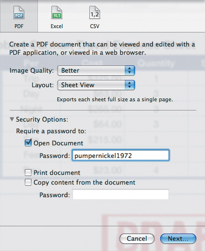
Because you want to export a PDF file, click the PDF button.
Choose an option from the Image Quality pop-up menu.
Good quality is acceptable for email attachments. Choose Better or Best for printing.
In the Layout pop-up menu, specify how you want to print each sheet.
Choose Sheet View so that the PDF will look identical to its Print View.
Click the disclosure triangle next to Security Options to choose options that make the document secure for sharing.
Select the Open Document checkbox to require a password to open the PDF.
Enter the password pumpernickel1972.
Click Next.
Specify a location in which to save your file.
You can target the chapter folder for temporary storage.
Click Export to save the PDF file.
If you want to share your spreadsheet with Microsoft Excel users, Numbers makes it easy to export your spreadsheet as an Excel document.
To make it easy to share iWork documents and collaborate with others, Apple created iWork.com. It’s essentially a web-based document-sharing service, but what it means to the iWork user is that you now have an easy way to post documents for review with a few clicks. This service is currently in beta, which means it’s still being developed, but is open to public trial. The service is currently free, and it allows others to view, comment on, or download your spreadsheet.
Choose Share > Share via iWork.com.
If this is your first time using the service on this computer, you’ll have to sign in.
Note
If you already have an Apple ID—from the iTunes Store, MobileMe, or the Apple Discussions forums—you can use that ID on iWork.com. If not, you must click Create New Account to sign up for a free Apple ID.
If necessary, enter your Apple ID and Password and click Sign In.

A new dialog opens and prompts you for important information required to share the file.
Note
You must be connected to the Internet to share a document with iWork.com Public Beta. You must also have a Mail account configured on your computer to send invitations to view the document.
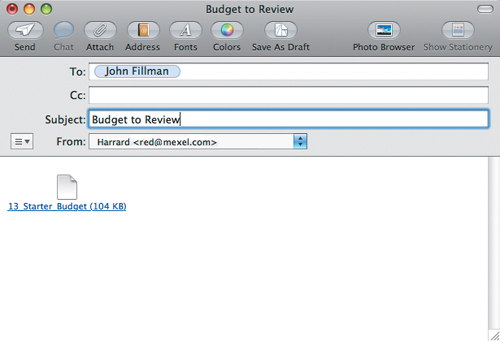
In the To and Message fields, enter the email addresses and any message you want to deliver to the recipients of the spreadsheet.
Modify the Subject field as necessary.
In the From pop-up menu, choose an email address to use for sending the invitation.
To enable viewer comments and downloads, keep the “Leave Comments” and “Download the document” checkboxes selected.
Tip
To set specific options for uploading and downloading files, click the Show Advanced button at the bottom of the sheet. Here you can choose which file formats to make available for download. The Upload options also let you specify the filename to be posted. If you are reposting a previously shared document, you can choose either to overwrite the old file or to enter a new name in the “Copy to iWork.com as” field.
Click Share.
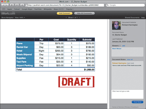
A copy of your spreadsheet is published to iWork.com. Unique invitations are sent to each individual you specified. The viewer can choose to leave comments and notes, or to download your spreadsheet.
You now know how to create and work with Numbers spreadsheets, as well as send them via email and share them via the Web.