The following figure shows a simple relational data model of a stock quote application:

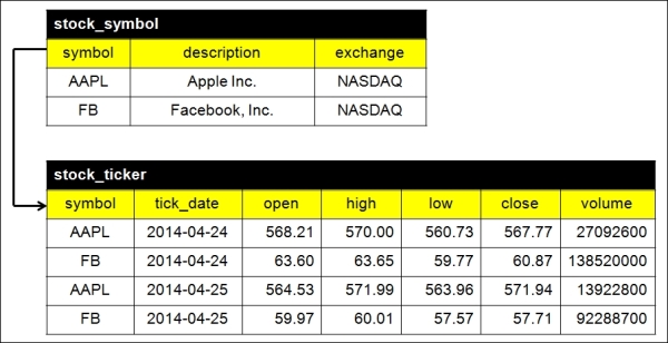
The relational data model of a stock quote application (Source: Yahoo! Finance)

The stock_symbol table is an entity representing the stock master information such as the symbol of a stock, the description of the stock, and the exchange that the stock is traded. The stock_ticker table is another entity storing the prices of open, high, low, close, and the transacted volume of a stock on a trading day. Obviously the two tables have a relationship based on the symbol column. It is a well-known one-to-many relationship.

The following is the Data Definition Language (DDL) of the two tables:

CREATE TABLE stock_symbol (
symbol varchar PRIMARY KEY,
description varchar,
exchange varchar
);

CREATE TABLE stock_ticker (
symbol varchar references stock_symbol(symbol),
tick_date varchar,
open decimal,
high decimal,
low decimal,
close decimal,
volume bigint,
PRIMARY KEY (symbol, tick_date)
);

Consider the following three cases: first, we want to list out all stocks and their description in all exchanges. The SQL query for this is very simple:

// Query A
SELECT symbol, description, exchange
FROM stock_symbol;

Second, if we want to know all the daily close prices and descriptions of the stocks listed in the NASDAQ exchange, we can write a SQL query as:

// Query B
SELECT stock_symbol.symbol, stock_symbol.description,
stock_ticker.tick_date, stock_ticker.close
FROM stock_symbol, stock_ticker
WHERE stock_symbol.symbol = stock_ticker.symbol
AND stock_symbol.exchange = ''NASDAQ'';

Furthermore, if we want to know all the day close prices and descriptions of the stocks listed in the NASDAQ exchange on April 24, 2014, we can use the following SQL query:

// Query C
SELECT stock_symbol.symbol, stock_symbol.description,
stock_ticker.tick_date, stock_ticker.open,
stock_ticker.high, stock_ticker.low, stock_ticker_close,
stock_ticker.volume
FROM stock_symbol, stock_ticker
WHERE stock_symbol.symbol = stock_ticker.symbol
AND stock_symbol.exchange = ''NASDAQ''
AND stock_ticker.tick_date = ''2014-04-24'';

By virtue of the relational data model, we can simply write different SQL queries to return different results with no changes to the underlying data model at all.

Now let us turn to Cassandra. The DDL statements in the last section can be slightly modified to create column families, or tables, in Cassandra, which are as follows:

CREATE TABLE stock_symbol (
symbol varchar PRIMARY KEY,
description varchar,
exchange varchar
);

CREATE TABLE stock_ticker (
symbol varchar,
tick_date varchar,
open decimal,
high decimal,
low decimal,
close decimal,
volume bigint,
PRIMARY KEY (symbol, tick_date)
);

They seem to be correct at first sight.

As for Query A, we can query the Cassandra stock_symbol table exactly the same way:

// Query A
SELECT symbol, description, exchange
FROM stock_symbol;

The following figure depicts the logical and physical storage views of the stock_symbol table:

The Cassandra data model for Query A

The primary key of the stock_symbol table involves only one single column, symbol, which is also used as the row key and partition key of the column family. We can consider the stock_symbol table in terms of the SortedMap data structure mentioned in the previous section:

Map<RowKey, SortedMap<ColumnKey, ColumnValue>>

The assigned values are as follows:

RowKey=AAPL
ColumnKey=description
ColumnValue=Apple Inc.
ColumnKey=exchange
ColumnValue=NASDAQ

So far so good, right?

However, without foreign keys and joins, how can we obtain the same results for Query B and Query C in Cassandra? It indeed highlights that we need another way to do so. The short answer is to use denormalization.

For Query B, what we want is all the day close prices and descriptions of the stocks listed in the NASDAQ exchange. The columns involved are symbol, description, tick_date, close, and exchange. The first four columns are obvious, but why do we need the exchange column? The exchange column is necessary because it is used as a filter for the query. Another implication is that the exchange column is required to be the row key, or at least part of the row key.

Remember two rules:

In a distributed system backed by Cassandra, we should minimize unnecessary network traffic as much as possible. In other words, the lesser the number of nodes the query needs to work with, the better the performance of the data model. We must cater to the cluster topology as well as the physical storage of the data model.

Therefore we should create a column family for Query B similar to the previous one:

// Query B
CREATE TABLE stock_ticker_by_exchange (
exchange varchar,
symbol varchar,
description varchar,
tick_date varchar,
close decimal,
PRIMARY KEY (exchange, symbol, tick_date)
);

The logical and physical storage views of stock_ticker_by_exchange are shown as follows:

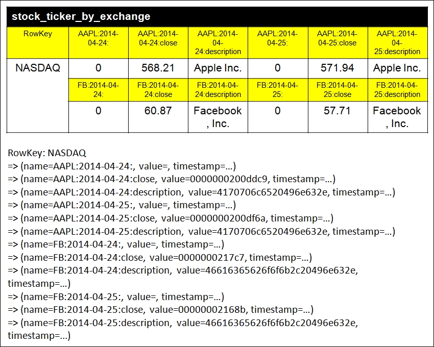
The Cassandra data model for Query B

The row key is the exchange column. However, this time, it is very strange that the column keys are no longer symbol, tick_date, close, and description. There are now 12 columns including APPL:2014-04-24:, APPL:2014-04-24:close, APPL:2014-04-24:description, APPL:2014-04-25:, APPL:2014-04-25:close, APPL:2014-04-25:description, FB:2014-04-24:, FB:2014-04-24:close, FB:2014-04-24:description, FB:2014-04-25:, FB:2014-04-25:close, and FB:2014-04-25:description, respectively. Most importantly, the column keys are now dynamic and are able to store data in just a single row. The row of this dynamic usage is called a wide row, in contrast to the row containing static columns of the stock_symbol table—termed as a skinny row.

Whether a column family stores a skinny row or a wide row depends on how the primary key is defined.

In either case, the first column in the primary key definition is the row key.

Finally, we come to Query C. Similarly, we make use of denormalization. Query C differs from Query B by an additional date filter on April 24, 2014. You might think of reusing the stock_ticker_by_exchange table for Query C. The answer is wrong. Why? The clue is the primary key which is composed of three columns, exchange, symbol, and tick_date, respectively. If you look carefully at the column keys of the stock_ticker_by_exchange table, you find that the column keys are dynamic as a result of the symbol and tick_date columns. Hence, is it possible for Cassandra to determine the column keys without knowing exactly which symbols you want? Negative.

A suitable column family for Query C should resemble the following code:

// Query C
CREATE TABLE stock_ticker_by_exchange_date (
exchange varchar,
symbol varchar,
description varchar,
tick_date varchar,
close decimal,
PRIMARY KEY ((exchange, tick_date), symbol)
);

This time you should be aware of the definition of the primary key. It is interesting that there is an additional pair of parentheses for the exchange and tick_date columns. Let's look at the logical and physical storage views of stock_ticker_by_exchange_date, as shown in the following figure:

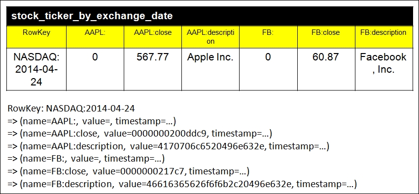
The Cassandra data model for Query C

You should pay attention to the number of column keys here. It is only six instead of 12 as in stock_ticker_by_exchange for Query B. The column keys are still dynamic according to the symbol column but the row key is now NASDAQ:2014-04-24 instead of just NASDAQ in Query B. Do you remember the previously mentioned additional pair of parentheses? If you define a primary key in that way, you intend to use more than one column to be the row key and the partition key. It is called a composite partition key. For the time being, it is enough for you to know the terminology only. Further information will be given in later chapters.

Until now, you might have felt dizzy and uncomfortable, especially for those of you having so many years of expertise in the relational data model. I also found the Cassandra data model very difficult to comprehend at the first time. However, you should be aware of the subtle differences between a relational data model and Cassandra data model. You must also be very cautious of the query that you handle. A query is always the starting point of designing a Cassandra data model. As an analogy, a query is a question and the data model is the answer. You merely use the data model to answer the query. It is exactly what modeling by query means.