
Most Likely Inference
Abstract
This chapter reviewed the connection of RELR to maximum entropy and maximum likelihood estimation methods. In particular, RELR was reviewed with respect to the principle of Jaynes which has origins in statistical mechanics. This Jaynes principle views the goal of estimation in complex systems to generate most likely inference given the available certain constraints measurements. RELR extends this principle to most likely inference given most likely constraints on measurements. This chapter reviewed how RELR's error modeling is a form of errors-in-variables regression which assumes that error exists in both independent and dependent variables. RELR's error modeling was then reviewed which makes three critical assumptions in addition to the assumption of independent observations. These assumptions concerned the existence of extreme value logit error, the equal probability of positive and negative errors across independent variable features, and that positive and negative error probabilities are unbiased across even and odd polynomial features. These assumptions were argued to be reasonable and allow the direct estimate of the logit error that standard logistic regression ignores.
Keywords
Bias; Binary variables; Boltzmann entropy; Cluster-specific effects; Correlated observations; Cross-sectional data; Cubic; Discrete choice; Dummy coded missing status variables; Errors-in-variables regression; Even polynomial features; Extreme value error; Extreme value type 1 distribution; Fixed effects; Gumbel distribution; Imputation; Continuous variables; Ratio variables; Interval variables; Jaynes Principle; Linear; Log likelihood; Logistic distribution; Logit error; Longitudinal data; Mixed logit; Most likely inference; Negative error; Normalization; Odd polynomial features; Ordinal variables; Panel data; Pearson correlation; Polynomial; Positive error; Power series; Probit regression; Pseudo-observations; Quadratic; Quartic; Random effects; Ranked variables; Ratio variables; RELR error model assumptions; Shannon entropy; Spearman correlation; Standardized variables; Statistical mechanics; Student's t; Taylor series; Transitional model; Welch's t
“A given system can never of its own accord go over into another equally probable state but into a more probable one…”
Ludwig Eduard Boltzmann, “The Second Law of Thermodynamics”, 1886.1
Contents
1. The Jaynes Maximum Entropy Principle
2. Maximum Entropy and Standard Maximum Likelihood Logistic Regression
3. Discrete Choice, Logit Error, and Correlated Observations
Boltzmann's concept of the Second Law of Thermodynamics necessarily assumed the existence of atoms. As a result, he spent much of his career arguing with the majority of his peers like fellow Austrian physicist Ernst Mach who vehemently disputed the existence of atoms. Boltzmann committed suicide in 1906 at the low point of atomic theory acceptance. Ironically, in just a few years after Boltzmann's death, experimental evidence was finally produced that led to the undeniable conclusion that atoms existed.2 Yet, it took many years after that for the atom to become part of the paradigm theory in normal science education. My father went to high school in a small town in the Midwest of the United States in the early 1940s where his elderly science teacher still taught that the existence of atoms was a controversial idea.
The Second Law of Thermodynamics is one of the great achievements of modern science. The modern understanding of this law is somewhat different from Boltzmann's understanding quoted above. It is that ergodic3 physical systems when isolated should be determined by laws of probability and be most likely to exist in maximum probability states. So, in the current understanding, a system may of its own accord go into other states besides a maximum probability state, but the maximum probability state is substantially more likely in complex physical systems with many particles such as ideal gases. The central concept of the second law is entropy as the most probable state is maximum entropy. The Boltzmann entropy expression is as follows:
![]() (2.1)
(2.1)
where S is the entropy, k is a scaling constant, and W describes the number of ways that particles can be arranged in terms of positions and momenta in space and time according to basic laws of combination. A system with greater entropy has more possible arrangements, so with greater entropy there is less information or more uncertainty in the actual arrangement.
In the middle of the twentieth century, Shannon was able to show that uncertainty is generally measured by an equation that has the same form as Boltzmann's entropy.4 Using the base e logarithm, the discrete form of Shannon's entropy H for a probability distribution p takes the form:
![]() (2.2)
(2.2)
where p(j) is the probability of an event across C possible outcome categories. So, in the case of a coin flip, C would be equal to 2 as these are just two possible outcomes. In that case, it is easy to verify that H(p) would be maximal when p(j) is equal to 0.5 for each of these two possible outcomes where the sum is constrained to equal 1. In that fair coin case where each of the two possible outcomes has equal probability, H(p) = 0.693. On the other hand, H(p) = 0.325 when one p(heads) = 0.1 and p(tails) = 0.9 or vice versa in biased coins. In general, H(p) is always less than 0.693 when p(heads) differs from p(tails). So, there is a maximal value of uncertainty H(p) about the outcome in a single coin flip when a head and a tail are equal in probability which makes sense. Shannon realized that with less uncertainty, there is always more information. Shannon's entropy expression is one of the cornerstones of information theory.
1 The Jaynes Maximum Entropy Principle
Soon after Shannon, Edmund Jaynes came to believe that because maximum entropy also reflects maximum probability, this suggests a very fundamental principle. In essence, he reversed the statistical mechanics problem that assumed that maximum entropy would be the most reasonable solution under assumptions about ergodic behavior in isolated systems and simply asked “what is the most probable behavior of a system given our historical observations and known constraints?” The answer Jaynes gave was:
… we take entropy as our starting concept, and the fact that a probability distribution maximizes the entropy subject to certain constraints becomes the essential fact which justifies the use of this distribution for inference.5
But Jaynes argued that this maximum entropy inference has much more general application than just in statistical mechanics, as he believed that the same principle always should be applied in every well-reasoned inference. In this general sense, Jaynes proposed that maximum entropy inference is always as much about the uncertainty that we have about our world than about anything else. Even to the extent that we can be certain in our constraints, we also must accept that there are other uncertainties related to what we do not know. So our measurements are likely to be incomplete because they are based upon finite data or do not include all constraints and thus there will be uncertainty in our knowledge. Yet, by maximizing entropy subject to certain constraints, this allows a most probable solution given incomplete information. The fundamental assumption is that all observations must be independent. This general principle of inference is now called the Jaynes maximum entropy principle.6
An understanding of this principle can be found in the simple example of inference that is possible in the case of the behavior of water molecules. Say that you have a closed container with liquid water at equilibrium where we measure the temperature. Now say that we open the system and add heat until the temperature reaches boiling, and the system is then closed again and at equilibrium. The added heat has caused molecules on average to increase in velocity, but we cannot say that any individual molecule has increased in velocity. This is due to the variability at any one point in time because some molecules might even be stationary as they stop momentarily when they run into each other. But at least in this case, one can characterize the most probable behavior of molecules by seeking the maximum entropy solution given the heat energy. We can develop probabilistic models that predict on average how an independent causal variable like heat may impact the probability that a given molecule may have specific behavior. This characterization only will be probabilistic and apply to average group behavior and not to individual molecules with certainty. But this can be even a causal inference under well-controlled comparison conditions that hold everything constant except for one changing causal factor. The tremendous insight of Jaynes was that this same principle could apply very generally to give most likely inference in all situations where uncertainty exists, and this even would include open systems and human behavior if applied correctly.
A naïve understanding of entropy assumes that a maximum entropy solution subject to all known constraints is necessarily a highly disordered pattern. But snowflakes are examples of a maximum entropy distribution of molecules subject to constraints. In snowflakes, a static maximum entropy distribution is frozen on the way to thermodynamic equilibrium that obeys constraints related to interactions between molecules and rate of freezing.7 In this case, these constraints impose strikingly low-entropy or high-information structure upon the resulting maximum entropy configuration. This low-entropy pattern is seen in the simple whole number harmonic ratios such as 2:1, 3:1, and 4:3 in the relative counts of the spikes and/or sides of the various embedded figures (Fig. 2.1).

Figure 2.1 One of the snowflakes photographed by Wilson Bentley. Notice the simple whole number harmonic ratios such as 2:1, 3:1, and 4:3 in the relative counts of the spikes and/or sides of the various embedded figures.8
Snowflakes are formed in open systems where entropy in molecular configurations is forced to decrease due to local environmental constraints. Biological systems like neural systems are also open systems, although like snowflakes they also can be assumed to exhibit stable maximum entropy phases subject to known constraints. For example, the Boltzmann maximum entropy distribution equation describes how the concentration gradient in the distribution of a charged molecule across the neural membrane is related to an electrostatic potential gradient in Hodgkin and Huxley's original explanation of the resting potential behavior of the neuron.9 Like the snowflake, this effect can be understood as a mechanism that maximizes entropy subject to known constraints. Like the snowflake, this is a clear example of the Jaynes principle that gives a most probable inference that explains a physical phenomenon.
In the neuron, most probable entropy decreases well beyond what would be expected in random behavior also can be represented as due to fundamental constraints in a maximum entropy inference system. For example, the membrane potential changes at the axon hillock that are graded potentials and change the probability of axonal spiking are caused by highly targeted synaptic and dendritic effects. Later in this book, it will be seen that these effects can be modeled as constraints in a maximum entropy formulation that is the RELR neural computation model. When these constraints are stable in the sense that the input features are fixed, the system will be most likely to produce the maximum entropy state subject to these input constraints. Later in this book, it also will be seen that very high information, small whole number frequency ratios of oscillating neural ensemble patterns can arise temporarily in the human brain during explicit cognition. These high information patterns are analogous to the low-entropy patterns of snowflakes.
In physical systems such as snowflakes and vibrating musical strings, simple harmonic relationships are easily understood as arising from stable orthogonal components in whole number frequency ratio relationships and easily analyzed with simple tools that assume that the harmonic frequencies fit perfectly within very regular analysis windows. But in complex systems that produce cognition and behavior, the problem is that perfect harmonic relationships are much more transient if they even exist. So, simple tools that force an assumption of stable low-entropy orthogonal relationships that fit perfectly within an analysis window like principal components analysis or Fourier analysis are not really effective and are more likely to force such relationships to exist when they are not in fact there. It is much better to use a method that does not force low-entropy structures that do not exist but will discover such structures if they do in fact exist, and the maximum entropy method is such a method.
2 Maximum Entropy and Standard Maximum Likelihood Logistic Regression
Although standard maximum likelihood logistic regression is probably the most popular approach in today's predictive analytics practice, many analysts do not know that it gives identical solutions to the maximum entropy subject to constraints method.10 Yet, the predictive features in standard logistic regression may be unlikely to be certain constraints unless determined through experimental means such as discrete choice methods. Thus, it probably would be a stretch to say that the widespread practice of standard logistic regression is always an application of the Jaynes principle of most likely inference.
In maximum likelihood logistic regression, observed outcomes in the form of binary dependent variable events are used to compute a function that estimates their probability of occurrence given the predictive features. This probability function is the joint probability that all observed outcome events occur. This is simply the product of the estimated probability of all observed outcomes just like the joint probability of independent coin flip trials is a product of the probability of all those individual outcome events. For example, the joint probability of two straight heads in a fair coin flip is 0.5 × 0.5 = 0.25, whereas the joint probability of three straight heads is 0.5 × 0.5 × 0.5 = 0.125. Again, this simple multiplicative joint probability rule does assume that the outcome events are independent events, so one event cannot cause or depend upon another event.
In software implementations, the logarithm of the likelihood is maximized in logistic regression because it is easier to compute. This Log Likelihood or LL of a probability distribution p is written as:
![]() (2.3)
(2.3)
where y(i,j) is the outcome for the ith observation in the jth category condition which is coded as “1” when an event occurs and “0” when an event does not occur. Similarly, p(i,j) is the estimated probability for the ith observation in the jth category condition. In a maximum likelihood solution, each p(i,j) is computed so that LL(p) is maximized. Notice that the log likelihood is simply the logarithm of the product or joint probability of all observed outcome events which are assumed to be independent.
For the binary case, there are two category conditions, so j = 2. So, with two coin flips, an instance of an event such as getting a head on a trial can be coded as “1” and a noninstance of an event such as not getting a head can be coded as “0”. If a head is observed on the first coin flip trial and a tail on the second, then the sequence is coded in terms of y(i,j) as 1, 0, or head/nontail for the first event and 0, 1 or nonhead/tail for the second event. In this case, then LL(p) = 1 × ln(0.5) + 0 × ln(0.5) + 0 × ln(0.5) + 1 × ln(0.5) = −1.386 because the maximum likelihood estimation would yield equal probability estimates p(i,j) for heads and tails. Unlike Shannon's entropy expression in Eqn (3.1) which always gives positive values, this log likelihood expression in Eqn (3.2) always gives negative values. Yet, just like the entropy measure, any probability estimates whereby p(heads) ≠ p(tails) would give lower log likelihood values. Because the probabilities that the maximum likelihood estimation generates are driven by empirical outcome event observations, they can be inaccurate in small or unrepresentative samples.
For a direct comparison to this log likelihood coin flipping example, in a binary outcome across N trials, Shannon's entropy can be written as:
![]() (2.4)
(2.4)
where p(i,j) is the outcome probability for the ith observation in the jth category condition. In a maximum entropy solution, each p(i,j) is computed so H(p) is maximized. If we take the case with two coin flips giving one head and one tail, we can compute the negative sum that gives the entropy as −0.5 × ln(0.5) + −0.5 × ln(0.5) + −0.5 × ln(0.5) + −0.5 × ln(0.5) = 1.386. So, notice that the entropy and log likelihood have the same magnitude, but opposite signs for the same probability distribution. This will be generally the case.
As in this example, it does not matter whether the entropy of the estimated probability distribution is maximized subject to constraints or the log likelihood is instead maximized. The very same estimated probability distribution simultaneously maximizes both objectives. With the exception of certain pathological cases, both maximum entropy and maximum likelihood logistic regression are also well-behaved optimization objectives where any local optimum is also a global optimum. One pathological condition is where perfect discrimination accuracy with zero error can be observed known as complete or quasi-complete separation, depending upon whether ties exist. In this case, there is no longer any unique optimal solution.11 Another pathological condition is that standard maximum likelihood logistic regression often fails to converge in the face of significant multicollinearity. We will see that RELR largely overcomes both of these pathological cases.
Whereas Shannon's entropy can be interpreted to measure uncertainty, a reasonable question is what does log likelihood measure in logistic regression? Since it is opposite in sign to uncertainty, log likelihood might be thought to be a goodness of fit measure which reflects the extent which a probability distribution matches the observed outcomes. Log likelihood gets greater or less negative as this match gets better and better. In general, a probability distribution which has a relatively higher or less negative log likelihood value would be a better match to data than one with a relatively lower or more negative log likelihood value. On the other hand, because entropy is opposite in sign to log likelihood, a higher value of entropy would be a poorer match to data and would be associated with greater uncertainty. So even though maximum entropy and maximum log likelihood generate the same probability distribution for the very same fixed set of predictive features, it is important to recognize that entropy and log likelihood have different meanings and will give different optimal values across changing predictive feature sets. For example, feature selection methods can be designed to discover the optimal objective function across many possible predictive feature sets, and the maximum entropy and maximum log likelihood solutions across these many possible feature sets normally would be different. In such feature selection optimization, both Implicit and Explicit RELR optimize maximum log likelihood functions for obvious reasons that are reviewed in the next chapter.
No matter whether it is computed through maximum log likelihood or maximum entropy, in logistic regression, the function that determines the estimated probability for each particular binary target outcome event follows a logistic distribution. That is, the probability of a binary outcome event at the ith observation and j = 1 and j = 2 categories is determined as follows:
 (2.5a)
 (2.5b)
where x(i,r) is the value of the rth feature at the ith observation, β(r) is the regression weight for the rth feature, and α is an intercept.12 The assumption that the distribution function is logistic is not the only way to get a maximum likelihood regression model with binary target outcomes. However, logistic regression is generally considered to be as accurate or more accurate and easier to compute than these other possibilities. Another older approach that is still sometimes used in econometrics is probit regression which assumes that this distribution function is normally distributed. Interestingly, probit regression and logistic regression give probability estimates that are almost indistinguishable,13 so standard logistic regression is usually used in this case simply because it is far easier to compute and much easier to interpret. Yet, logistic regression also has a basis in information theory through its equivalence to maximum entropy, and this might be its greatest theoretical advantage.14
The practical interpretation advantage of logistic regression is seen in the nice linear form of the logit or log odds, as probit regression has no comparable way to interpret odds so easily. From the probability value p(i,j), this logit or log odds of a binary event in the ith observation and jth category easily can be derived which is
![]() (2.6)
(2.6)
or for j = 1,
![]() (2.7)
(2.7)
This logit definition in Eqn (2.7) has the same form as an ordinary linear regression equation although there is no error term. Like linear regression, the features in the logit are independent variables that combine in a linear additive manner and also can be nonlinear and interaction effect terms, so a logit model that arises from logistic regression is not limited just in terms of linear main effect features. Like ordinary linear regression, a problem with standard logistic regression is that overfitting error and related multicollinearity error occur as more features are added, and this can be especially problematic with nonlinear and interaction effects. When overfitting and other related multicollinearity error occur in standard logistic regression applications, such error is a sign that the Jaynes principle that maximum entropy gives the most probable inference cannot be applied. This is because the Jaynes principle only applies to the case where certain constraints are entered into a model and overfitting error is clearly a case where unknown or unfounded independent variable constraints are entered in a model. In reality, there is almost always significant error in the logit estimate in standard logistic regression due to incorrect data values, multicollinearity, overfitting, omitted variables, missing data, sampling, outliers, and rounding. While this logit error is not a parameter that is ever estimated in standard logistic regression, it still has been intensively studied in one major application area. This is discrete choice modeling.
3 Discrete Choice, Logit Error, and Correlated Observations
Discrete choices are decisions involving two or more alternatives such as whether to vote for the Republican or Democratic candidate, whether to take a plane or ride a bus, or whether to take a job or not. While not all person attributes can be experimentally manipulated in a choice study, a researcher often can vary the attributes associated with a choice experimentally such as the price or quality of product to be purchased, and determine causal effects on the decisions. At least with these choice attributes where randomized experiments are possible, reasonably certain predictive features may be selected in a model in accord with the Jaynes principle. However, besides predictive features that a researcher can test and select experimentally, it is likely that other important unobserved constraints will have an impact. So, discrete choice models are subject to significant logit error problems due to unobserved constraints.
Discrete choices are most often assumed to be based upon a process whereby decision makers choose an alternative that maximizes their utility or net benefit given the attributes of a decision. One view known as causal decision theory is that such utility directly reflects causal determinants of behavior, whereas another evidential view is that it only reflects a conditional probability which is sometimes only correlational. Given the very same decision variables and historical learning, these two utility processes often generate the same optimal decisions. However, there are some interesting scenarios where the evidential theory would predict that you would do that which you would be happiest to learn that you have done, whereas the causal theory would predict that you would do that which is most likely to bring about good results.15 Causal decision theory is more consistent with decisions that are under conscious or explicit control. Evidential decision theory is more consistent with decisions that are not under conscious causal control. Still, unconscious or implicit choices might be immediately available to consciousness after they are made. The view of this book is that both explicit and implicit processes are important in all phases of human cognition including decisions, so the present view is that both causal and evidential decision theories may each reflect an aspect of decision processing. However, decisions that are guided by causal understanding would be viewed as better decisions and less risky, although there are certainly exceptions related to the need for speedy decisions in stable environments where causal understanding is not such an important factor.
Under either the causal or the evidential theory, if a person is given a choice between taking a plane or riding a bus to a distant city, and if the person is poor and only has the money for a bus ride and also has the time to ride the bus because they are unemployed, the utility associated with the bus alternative would be likely to be higher than that associated with the plane. So, if a researcher observed such a person's decision and also was certain of their employment status and savings, then one could predict that the bus alternative would have greater utility than the plane alternative. The problem arises when factors that determine a decision are not observed, as there may be error in the model's prediction due to unobserved factors.
Since the pioneering work of Nobel Laureate Daniel McFadden,16 discrete choice has been traditionally modeled through standard logistic regression where the alternatives are response categories and the choice and decision maker attributes are predictive features. The utility or U(i,j) that the ith decision maker assigns takes the identical form of the logit17 so for the j = 1 binary category alternative in a discrete choice model, this becomes
![]() (2.8)
(2.8)
This is exactly the same form as Eqn (2.7) and the indices have similar meaning, but there is the addition of the error term ε(i,1). In the most general form that still maintains the linear additive characteristics of each individual feature value x(i,r) being multiplied by a regression weight β(r) and then summed, the features in the choice model given by the vector x may be attributes of a choice, attributes of a person, along with interactions and nonlinear effects. In the binary discrete logit choice model with just two categories, the error term ε(i,1) is not estimated directly and is treated as random just like how ordinary linear regression does not estimate its error term and treats it as random. It represents the errors associated with the jth (j = 1) binary alternative relative to the reference alternative (j = 2) for the ith decision maker. As suggested above, standard logistic regression discrete choice modeling assumes that such modeling error would arise due to the failure to include certain constraints, or what may be called unobserved factors that influence an outcome, along with other forms of measurement error. There is almost always uncertainty because the discrete choice probability estimates seldom match the actual choice responses closely for all observations, so the error term ε(i,1) is designed to represent this uncertainty formally. Figure 2.2 shows a standard logistic regression model's probability estimates p(i,j) for the j = 1 binary alternative across i = 1 to N observations, along with the actual binary choices 0 or 1. There is a nontrivial amount of error in the logistic regression model's probability estimates for these choices, as the regression model only provides a best or maximum likelihood fit.

Figure 2.2 Example of substantial error that is usually seen in logistic regression models. The gray curve reflects the probability of the responses, whereas the black curve reflects binary (0, 1) responses across 14 consecutive trials in simulated data. The error that is defined in discrete choice modeling is represented by the difference between these two curves.
A critical assumption in discrete choice standard binary logistic regression modeling is that the modeling error that results from unobserved factors in the j = 1 alternative is independent from that in the j = 2 alternative.18 This assumption that the error is independent in the j = 1 and j = 2 binary choice alternatives would seem realistic in cases where only one observation is measured from each decision maker in a sample of independent decision makers who have no influence upon one another. In such a case, unobserved factors would be present and independent across the two observed binary outcomes because all observations would be independent.
This assumption of independent error might be problematic in other situations where observations are not entirely independent such as when multiple responses are sampled from the same individual decision makers over time. For example, it might be that later responses tend to be only in one alternative versus another due to a drifting response bias where error in one alternative is not independent of error in another alternative. So in standard logistic regression binary choice modeling, the assumption of independent error can be restrictive in situations where there are unobserved causal factors that produce significant serial correlation in response data as reviewed by Kenneth Train.19
Unfortunately, the attempts to control for correlations in observations without any sense of causal relations can lead to incorrectly specified and problematic models. For example, the Generalized Estimating Equation (GEE) method has been used as a way to handle correlated observations in logistic regression in what are termed population average models in the biostatistics literature.20 Yet, this method requires that a researcher specifies the correlation structure between observations, or it will automatically generate such correlation structure with a resulting unwieldy number of parameters with many likely spurious correlations. Because of such large number of parameters, many researchers prefer to specify this correlation with very simple structures that are constant over time. It has been argued that incorrectly specified correlations in GEE will hurt the efficiency of the model, yet it is also argued that the model will still be consistent in the sense that with enough data, the solution will be the same as that which would be obtained with correctly specified correlation structure. Still, there is no guidance on how much data is needed for such consistency. In fact, there can be suspicious problems in GEE in epidemiological studies which are likely due to incorrectly specified time varying covariates.21
Other popular methods to deal with error due to correlated observations in standard logistic regression involve some aspect of fixed effect or random effect designs. In these cases, assumptions must be made about whether to treat error due to correlated observations across repeated measures as fixed versus random with strict assumptions involved in each case. When fixed effects are assumed, intercepts or equivalent differencing must be introduced to account for correlated errors due to the distinct clustering units such as stores, schools, and hospitals. These estimated effects along with their interactions can have substantial error. Even more problematic is that fixed effect designs do not allow the estimation of between-subject explanatory effects. For example, between-subject effects like gender effects cannot be assessed as fixed effects in a longitudinal study of observations from the same persons over time because fixed effects are only sensitive to within-person effects that change over time in such a design. In fact, only within-subject effects that change significantly over time can be estimated. But, within-subject effects typically do not have the same variability as between-subject effects, and this makes their estimation more difficult.
As is commonly used, a random effects design usually means that a normally distributed random intercept with a mean of 0 and standard deviation of 1 is forced to occur across higher level clustering units such as schools, although any distribution is theoretically possible.22 When random effects are assumed in logistic regression modeling, lower level between-person explanatory effects like related to characteristics of students can be estimated but only with the very restrictive assumption that these effects are uncorrelated with the random effects used to model higher level clustering units such as schools. Otherwise, bias will be present. These biased estimates are also not consistent, so they would not be corrected with larger samples that approach the population. This random effects assumption can be quite controversial. Yet, mixed effects designs which require researchers to assume aspects of both fixed and random effects are frequently used with observation data even when the random effects assumption is dubious. This is probably because there have been no other good options.23
Kenneth Train comments that the assumption in discrete choice models of independent errors over time often has severe restrictions.24 To avoid this assumption, he proposes that one may consider using probit or mixed logit designs in discrete choice models. While probit regression often can lead to reasonable estimates, Train warns that the assumption of normally distributed error can lead to wrong signs in certain types of variables such as price. Train also suggests that the proposed probit computation that potentially allows correlated errors over time is complex, so researchers have more recently simply made the assumption that errors are independent over time in probit models. In contrast, he suggests that the mixed logit does not require special computation that is more complex than other aspects for models that assume that error is not independent. Yet, mixed logit is a random effects model and requires the same assumptions as detailed above and also requires a researcher to specify a probability distribution to characterize the error.25 Because of this, mixed logit has been described as being best suited for high-quality data26 which presumably would always have to be experimental data. In addition, there is quite a long list of model specifications in mixed logit necessarily under the control of the researcher that can have a very large effect on model quality,27 and these could be influenced by human biases.
In many cases, Train argues that unobserved factors that produce serial correlation can be modeled correctly in standard logistic regression with completely independent observations. For example, one binary dependent variable outcome that leads another by one observation or y(i − 1,j) may be introduced into a model and be a putative causal attribute for observed serial correlation such as related to habit formation in the case of positive serial correlation or a variety seeking personality in the case of negative correlation. In the biostatistics literature, these kinds of models are called transitional models, which are based upon longitudinal studies where previously measured outcomes can be used as covariates in new cross-sectional or cohort samples where all observations are still independent.28 These transitional models do not allow the degree of control that is possible with experimentally manipulated factors in randomized controlled experiments. So even in the most controlled situation in discrete choice experiments, some reliance on less controlled observation factors might be necessary if one wishes to avoid unobserved factors. The larger problem is that the error due to unobserved factors is really just one of many possible types of measurement errors that could have a major effect on the quality of the model.
4 RELR and the Logit Error
There is a long tradition in linear regression research on the effect of measurement error in both independent and dependent variables.29 The error-in-variables problem was also first extended to logistic regression many years ago.30 This work showed that in realistic scenarios where measurement error would be expected in both dependent and independent variables and unobserved effects are present, both standard linear and logistic regression models would produce biased regression coefficients that do not reflect true regression coefficients even when the constraints that are considered are certain and independent observations are present. This work also showed that such bias would not be alleviated by larger samples. So regression coefficient estimates are not consistent under realistic scenarios where not all independent variable constraints are measured or where measurement error exists in both dependent and independent variables even with perfectly independent observations.
How does this square with the Jaynes principle? It suggests that there are limits to what we can know with standard regression methods even when we know a subset of the true constraints with certainty because our regression estimates will still be biased unless the error is uncorrelated with the measured known independent variable constraints. Like the discrete choice modeling research, these derivations and simulations on error-in-variable effects do not even consider all sources of error. However, this work does include measurement error due to sampling, underfitting error due to unobserved factors, and multicollinearity error in the sense that an unobserved factor can bias regression coefficients in observed factors.31 Yet, overfitting error is another obvious other source of error, as well as multicollinearity error in measured independent variables. So the news is not good for standard regression modeling in respect to the Jaynes principle because the most likely inference still may not be a very good inference even with perfectly independent observations and certain independent variable constraints in the face of other significant sources of error. The only occasion where standard regression methods might avoid these problems would be where there are orthogonal independent variables and little measurement error in both independent and dependent variables.
In binary logistic regression or ordinal logistic regression with very few ordinal categories, measurement error in the dependent variable is much less of a problem because there are very few dependent variable values. This dependent variable error can be expected to subside approximately as an inverse square root function of the sample size, and is reflected by intercept error.32 So at least with a large enough sample so that variation in the proportion of target responses in different response categories can be expected to be small, one can ignore intercept error as a significant source of error in logistic regression. Yet with all other sources of error, one needs to assume that the aggregate effect of all error will be uncorrelated with estimated regression effects. Effectively, this assumes that the error will sum to zero in standard logistic regression.
This assumption of no error in independent variable effects is very unrealistic. A much more realistic regression model would estimate parameters which reflect error in the independent variable effects as a component of the regression. Yet, standard error-in-variables methods must make reasonable assumptions about error, or else the models will become an artifact of those assumptions. For example, one problem with common error-in-variables methods in linear regression is that an assumption of the ratio of error in the dependent variable to the error in each independent variable is required.33 But, this is not usually knowable. So, realistic assumptions that are knowable need to be at the heart of any error-in-variables method like RELR.
As an error-in-variables method, RELR starts with a more realistic assumption than standard logistic regression that significant error always will be present due to a wide variety of unknown error sources, but it specifies error modeling parameters designed to estimate the probability of this error. In fact, standard logistic regression can be considered to be a special case of RELR when all error that RELR models is zero. That is, as reviewed in the RELR formulation presented in Appendix A1, the log likelihood expression for RELR can be written as follows:
![]() (2.9)
(2.9)
where this log likelihood combines two probability distributions p and w.34 The first component is reflected by the left most set of summations in Eqn (2.9) involving the outcome probability distribution p. This is called the “observation log likelihood” or OLL, as it reflects the log likelihood corresponding to the observed dependent variable outcome events y(i,j) across the i = 1 to N observations and j = 1 to C categories. This first component is identical to the log likelihood expression in standard maximum likelihood logistic regression shown in Eqn (2.3). The second component in RELR is the second set of summations across the error probability distribution w. This component is unique to RELR, and is called the “error log likelihood” or ELL. It reflects the portion of the RELR model that relates to error modeling. The entire LL(p,w) expression in Eqn (2.9) can be called the RLL or the “RELR log likelihood”. The observations indexed as y(l,j,r) in the RELR error model are pseudo-observations designed to reflect inferred error across the l = 1 to 2 positive and negative error conditions, j = 1 to 2 error modeling categories and r = 1 to M independent variable feature constraints.35 As reviewed in Appendix A1, the number of categories C in the left hand summations would only be different from 2 in the case of when RELR models ordinal category dependent variables, but summation across the error modeling categories in the right hand summations always should be for j = 1 to 2. This is because RELR's ordinal regression is similar to proportional odds ordinal regression, which has identical properties to binary logistic regression except for multiple intercepts. The proportional odds assumption is required in RELR's ordinal regression.
This RELR error model is in the spirit of the Jaynes principle which assumes that the inclusion of known constraints can greatly aid in reducing uncertainty and thus lead to a more likely inference. The basic idea that motivates RELR is that the constraints that determine the error in the logit are known at least in an aggregate sense. These constraints dictate that one need not be concerned about error in the dependent variable or intercept error which can be assumed to be negligible with a large enough sample. So RELR does not attempt to estimate intercept error, as the error modeling in RELR can be assumed to reflect error related to all sources other than intercept error. Both positive and negative errors are inferred always to be present to some degree. In this formulation, parameters that capture the effect of error are now directly estimated. As derived in Appendix A2, the RELR logit for the j = 1 binary outcome at the ith observation can be derived from consideration of the joint probability of this outcome and all errors in variables across all r = 1 to M features and can be written as follows:
![]() (2.10)
(2.10)
where it is recognized that the far left hand summations involving the error terms cancel to zero given the definition of the error probabilities provided in the appendix. This is comparable to the standard logistic regression logit defined in Eqn (2.7) except that the logit error is now estimated for the l = 1 and two positive and negative errors across the r = 1 to M independent variable features, so RELR will almost always return different regression coefficients β(r) due to this error-in-variables adjustment. The utility U in Eqn (2.8) is also a logit with an error term similar to RELR's logit in Eqn (2.10), but this error in binary discrete choice utility modeling ε(i,1) is undefined and not estimated. So RELR decomposes and estimates this logit error for each dependent variable category in terms of positive and negative error components that exist for each independent variable feature, whereas discrete choice has traditionally viewed this error as a quantity that cannot be estimated.
A very key assumption in RELR is identical to that in standard maximum likelihood logistic regression. This is that all observations are independent, so dependent variable responses in one observation cannot cause or depend upon dependent variable responses in another observation. Normally great care must be taken to ensure that this assumption is fulfilled though proper sampling design. RELR's error modeling deals effectively with multicollinearity error in dummy coded variables that represent clusters of correlated observations. Still, in all cases it must be assumed that one outcome observation cannot cause or depend upon another outcome observation. This assumption is not often the case in longitudinal data, but transitional models are possible where covariate effects may be based upon outcomes from previous samples, and an example will be shown in Chapter 4. Because RELR allows very small sample models due to its error modeling, knowledgeable researchers and statisticians can find ways to fit models within RELR's independent observations requirements.
Along with this independent observations assumption, RELR's error modeling directly results from the following three assumptions concerning the logit error that is shown in Eqn (2.10):
1. Across independent variable features, positive and negative logit errors are independent and identically distributed Extreme Value Type I random disturbances with the expected positive and negative errors for each independent variable feature being inversely proportional to t.
2. Across independent variable features, the probability of positive and negative errors is equal.
3. Across independent variable features, the probability of positive and negative errors is not biased by whether features have an odd or even powered exponent in a polynomial expression.
In the first assumption, t is a t-ratio statistic that describes the reliability of the correlation of the rth independent variable feature with the dependent variable. This expected error that is inversely proportional to t for each feature is scaled by the sum of all such t values across all M independent variable features and multiplied by 2 to reflect independent positive and negative error estimates as shown in Appendix A1. This scaling has the effect of normalizing the inverse expected error which becomes the expected proportional effect so that the sum across positive and negative errors for all features is simply unity. The expected logit error serves as a naïve prior error, as the actual estimated error may differ substantially from this expected error. The 1/t expected error gives extreme expected values of error when t is small in magnitude, so it is consistent with the Gumbel or Extreme Value type 1 error that has been shown to characterize the logit error in standard maximum likelihood logistic regression discrete choice derivations.36,37 This logit error arises from the demonstration that the difference between two Gumbel extreme value distributed measures is distributed logistic.38 In the case of RELR, the positive and negative estimated errors in the logit then can be thought to be the two Gumbel extreme value measures that give rise to a difference which is the actual error which is distributed logistic.
In fact, this 1/t expected error fits all known relationships between the Student's t distribution, the logistic distribution, and the Gumbel extreme value distribution to a very good approximation. For example, the choice of t in the RELR error model is not arbitrary, as the Student's t-distribution and the standardized logistic distribution are essentially the same distribution.39 In addition, as shown in Appendix A1, when the two RELR extreme value distributed variables—positive and negative logit errors for a given feature—have their expected error, their difference gives a standardized RELR logit coefficient for that given feature that is approximately proportional to Student's t.40 Hence, the choice of expected error as being proportional to 1/t across features gives all known relationships between extreme value error variables, the logistic distribution, and the Student's t-distribution. Another choice for the expected error such as 1/t2 would not preserve these known relationships and instead give an anomalous result such as a proportional relationship between standardized logit coefficients and t2 instead of t. This would be inconsistent with the result that the difference between two extreme value variables has a logistic probability distribution. Thus, the choice of 1/t in the RELR error model is not arbitrary, although it is only a good approximation given that the Student's t-distribution and the logistic probability distribution are only approximately equivalent.
Pearson correlations are used because they have general application across ratio, interval, ordinal and binary level measurements. For example with ordinal variables, Pearson correlations give identical correlations to Spearman correlations when ranked variables are employed, so the coding of ordinal variables into ranked values is the best practice prior to using such variables. Binary variables conveniently produce identical correlations whether they are interpreted as ordinal variables and coded to reflect a rank with Spearman correlation or ratio variables that reflect a probability of 0 or 1 as with Pearson correlation, so there is no need to code binary variables into ranked variables. RELR standardizes all independent variable features to have a mean of 0 and a standard deviation of 1, and missing values are imputed as 0 after the standardization and after dummy coded missing status variables are also employed. The t value that reflects the reliability of the Pearson correlation needs to be computed prior to imputation. When this is done, the 1/t expected error gives greater error for features with more missing values everything else being equal which has validity and is quite different from how mean-based imputation typically works. Note that RELR's handling of missing values does not force an assumption of values that are missing-at-random. Even though the mean-based imputation by itself is based upon this assumption with zero information added so the imputation which guards against incorrect guessing of values, the dummy coded missing status features would be sensitive to structurally missing data that are not missing at random. Thus, these dummy coded missing status features can adjust any associated imputed features accordingly if structural missing data have an effect in a model. In contrast to RELR's imputation, multiple imputation can generate significant error if missing-at-random assumptions are not true.
The t values that reflect the reliability of the Pearson correlation between an independent and a dependent variable are generally suited to the error modeling based upon combinations of ratio, interval, ordinal and binary variables. However, independent sample t-tests that compare mean differences in binary groups give almost identical values with balanced samples. Unless the training sample size is very small,41 a best practice is always to use balanced stratified samples where there are an equal number of nonreference and reference target observations. With such balanced samples, the independent samples t value is not dependent upon the variance estimate calculation, as independent samples Student's t and Welch's t values are identical and they are also approximately identical to the t values based upon the Pearson correlations. In fact, balanced stratified sampling has become a standard approach in logistic regression modeling where intercepts are corrected at the scoring stage to reflect actual estimated imbalance in the relative proportion of binary outcome responses. So the best RELR practice of sample balancing accords with this already existing standard approach in logistic regression modeling.
Actual positive and negative errors always cancel each other to some extent, but this net error that results from the difference between the estimated positive and negative errors is the quantity that can be estimated through the logistic distribution in RELR. These positive and negative errors are assumed to be random variables, so there should be no greater probability of positive versus negative error for a given set of features. So, the second assumption assumes that the probability of positive and negative error are equal across features in the training sample used to build the model.
The third assumption relates to how RELR defines features. In RELR, an input variable is standardized with a mean of 0 and a standard deviation of 1 to define the linear feature and then all higher order polynomial and interaction features are computed based upon this standardized linear feature and then also standardized. This produces very different nonlinear and interaction effects than what would be observed based upon raw variables that are not standardized. For example, because all RELR variables are defined on the same standardized scale, they are not subject to the marginality problems where predictions may change with interaction and nonlinear effects simply based upon the scaling when there is arbitrary relative scaling of features.42 Additionally, with raw unstandardized variables, features of the same input variable based upon polynomial terms with odd exponents are almost perfectly correlated to features based upon even exponents. Yet, there is almost no correlation between the odd and even polynomial features for the same input variable with the standardized features used in RELR. Thus, the reason that odd and even polynomial features are grouped separately in RELR is that these standardized linear and cubic features are very highly correlated as are standardized quadratic and quartic features where Pearson's r is typically >0.9 in each group, whereas correlations across groups are typically <0.1. This correlation grouping that separates standardized odd powered and even powered polynomial features is already obvious with as few as 10 observations in the simulated data shown in Fig. 2.3(a)–(c).

Figure 2.3 (a–c) Examples of correlation with as few as 10 observations between features of input variables in RELR's standardized variables. Standardized features with odd powered exponents (linear and cubic) are always highly correlated, whereas standardized features with even powered (quadratic and quartic) exponents are also highly correlated. These correlations average >0.9 in larger samples. However, odd power features do not correlate highly to even power features with correlations averaging below <0.1 in larger samples. An equal weighting of causal features in top panel and random noise signal that varied between −4 and 4 in the logit were used in a logistic regression forward model where any probability ≥0.5 = 1 and <0.5 = 0. Features in middle and bottom panels are spurious to this simulated binary outcome signal. See Fig. 2.4(a) for more details of simulation methods.
The third assumption in RELR's error model takes the second assumption of equal probability of positive and negative errors and applies it separately to odd (linear and cubic) versus even (quadratic and quartic) polynomial features. The result is that there is no bias to have a greater positive versus negative probability of error in independent variable features with even powered exponents compared to terms with odd exponents. This third assumption needs to be imposed as a constraint in the RELR model because there is naturally a tendency for correlations and t values to be larger for standardized polynomial features with even powered exponents compared to odd powered exponents, and this can have a biasing effect on the error model which is based upon t values which reflect correlations to the dependent variable.
Bias across polynomial effects has been reported previously in simulated datasets that have multicollinear relationships between independent variables.43 However, the precise pattern of bias will depend upon whether raw versus standardized features are used and how the standardization is performed. The pattern of bias in the expected 1/t error across RELR's standardized polynomial features can be inferred from Fig. 2.4(a) which shows how the t values vary across the four components (linear, quadratic, cubic, and quartic) in a binary logistic regression forward simulated model where the logit was composed of an equal mix of all four components. Quadratic and quartic features give larger magnitude t values than linear and cubic features. This difference is quite substantial being almost exactly two times larger on average, and very reliable across all 30 simulation trials with each trial composed of 1000 independent observations as shown in Fig. 2.4(a).
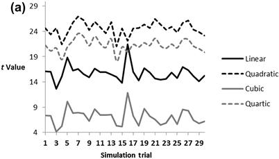
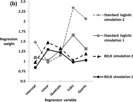
Figure 2.4 (a) Example of bias in t value patterns that is reliably observed across linear, quadratic, cubic and quartic t values created by employing a random number generator where signals varied between 0 and 1 to produce the linear feature x which was then mean centered and standardized. This is a representative sample of 30 trials of a simulation which consisted of an equal mix of each feature in a logistic regression forward simulated model where y = exp(xs + (xs2)s + (xs3)s + (xs4)s − ln(0.29))/(1 + exp(xs + (xs2)s + (xs3)s + (xs4)s − ln(0.29))) and where each polynomial feature is not a raw variable but instead is a standardized variable with a mean of 0 and a standard deviation of 1 and the subscript s is used to remind readers of this standardization and its order as the nonlinear features are each created from the standardized linear feature xs and then also standardized. In this simulation, a binary signal was created where any y value ≥0.5 was coded as 1 whereas any value <0.5 was coded as zero across 1000 observations similar to the simulation described in Fig. 2.3(a)–(c) but with a much larger sample and no random error signal was used here. The intercept of −ln(0.29) was used because it gave approximately equal numbers of 0 and 1 signals. This binary signal was then correlated to each particular polynomial feature that was an independent variable feature and the t values for each feature and each simulation trial was determined. Clearly, even polynomial features tend to produce larger t values. (b) Comparison of RELR models versus standard logistic regression models in two simulations across 1000 observations created exactly as described for Fig. 2.4(a) except that a random number generated noise signal that varied with equal probability between −2 and 2 was now added to the forward logistic regression described in Fig. 2.4(a) to ensure maximum likelihood convergence in standard logistic regression. Clearly, the RELR models have greater weight in linear and quadratic and lower weight in cubic and quartic signals, whereas this bias is opposite for standard logistic regression. There is also substantially more instability (greater variability across the two simulation samples) in the Standard Logistic Regression weights compared to the RELR weights.
Figure 2.4(b) shows two corresponding RELR and logistic regression models generated with simulated features described in Fig. 2.4(a) and with a random error signal designed to ensure that complete or quasi-complete did not occur so maximum likelihood convergence would occur. The RELR models do have a slight bias toward linear and quadratic effects relative to cubic and quartic effects, and this bias is reversed and more substantial in standard logistic regression models. However, the RELR models are more stable than the standard logistic regression models.
Without a nonbiased constraint to impose the third assumption, RELR's estimated expected error 1/t would be much higher on average for linear and cubic features. As a result, there would be a bias toward the selection of more false-positive effects in even power features relative to features that result from odd power exponents. RELR avoids this bias with the nonbiased constraint which forces the probability of positive and negative errors to be equally likely across features without any bias toward linear/cubic versus quartic/quadratic features.
With larger samples like the 1000 observations that were the basis of Fig. 2.4(a), another obvious pattern emerges. This is that there is a falloff in the sensitivity of t values with t values being more sensitive to linear features than cubic features and more sensitive to quadratic features than quartic features. The result is that RELR's expected error based upon inverse t values is biased to be lower with linear and quadratic effects than to cubic and quartic effects, so linear and quadratic effects would be more likely. This is especially true when the signs of the higher order cubic and quartic effects are reversed in simulations which only include causal linear and cubic features or only include causal quadratic and quartic features as shown in Fig. 2.5(a) and (b).
Figure 2.5 (a) and (b) Example of bias in t value patterns that is reliably observed across Linear, Quadratic, Cubic and Quartic t values in simulation which only included some features (causal) but estimated all features (noncausal features are labeled spurious). This simulation was also different from Fig. 2.4(a) in that the higher order cubic and quartic causal features were reversed in sign. The top figure is a representative sample of 30 trials of a simulation which consisted of an equal mix of each causal feature in a logistic regression forward simulated model where y = exp(xs − (xs3)s)/(1 + exp(xs − (xs3)s)) and where each polynomial feature is not a raw variable but instead is a standardized variable with a mean of 0 and a standard deviation of 1 and the subscript s is used to remind readers of this standardization and its order as the nonlinear features are each created from the standardized linear feature xs and then also standardized. In this simulation, a binary signal was created where any y value ≥0.5 was coded as 1 whereas any value <0.5 was coded as zero across 1000 observations similar to the simulation described in Fig. 2.4(a) but also notice sign reversal of causal features in simulation. This binary signal was then correlated to each particular polynomial feature that was an independent variable feature and the t values for each feature and each simulation trial was determined. The bottom figure was produced similarly but only even polynomial terms were causal, so y = exp((xs2)s − (xs4)s)/(1 + exp((xs2)s − (xs4)s)). Notice that lower order causal features—linear and quadratic—clearly give larger t-value effects.
RELR does not attempt to correct for this particular bias that favors lower order linear and quadratic effects to have greater magnitude. Bias always will be a part of quantitative descriptions of reality because there is no perfect filter which has equal sensitivity to all aspects of the world. Instead filters necessarily must focus on some aspects of the world while diminishing others. The hope is that quantitative filters result in predictions and explanations that are similar to how human brains work. Human brains prefer to think in terms of simpler effects. That is, linear effects are preferred over cubic effects, and quadratic effects are preferred over quartic effects. This is because the human brain has a much easier time understanding simpler quantitative relationships. Even if a causal effect is more accurately described with cubic or quartic effects, most scientists would prefer to report a linear or quadratic effect if they fit data approximately almost as well. That is exactly what RELR does with its natural bias toward simpler effects.
In full models where parsimonious feature selection is not attempted, RELR is incapable of resolving linear versus cubic effects or quadratic versus quartic effects as separate effects often, but will have a bias toward placing greater magnitude weights on the lower order polynomial effects. In parsimonious feature selection models, this will mean that RELR will be much more likely to select linear and/or quadratic effects. This bias might be considered to be an advantage to RELR as it seems similar to what the human brain would be most likely to communicate on its own. Of course, if there is a very strong cubic or quartic effect that drowns out the lower order polynomial power effect, then RELR will observe such an effect.
While current software implementations only include polynomial terms up to the quartic effect, it is obvious that RELR could be applied in applications which employ much higher order polynomial features. Many important functions like sine and exponential functions can be approximated by a series of polynomial terms that includes higher order features in a Taylor series expansion over a defined interval. In fact, the Taylor series to approximate a sine function on the interval between −π and π has as its first two terms x and −x3/6 which is exactly what RELR gives back from the simulation in Fig. 2.5(a) as its expected standardized effects which are in fact the t values as reviewed above. This is because the means prior to standardization are roughly zero, whereas the standard deviations prior to standardization are roughly twice for the cubic versus the linear RELR effect (Fig. 2.6(a) and (b)). On the other hand, t value effects are three times larger for positively weighted linear standardized versus negatively weighted cubic standardized variables (Fig. 2.5(a)). This implies that the −x3 variable is divided by twice the linear term, whereas its expected effects once standardized are one-third the linear term. So the value in the denominator becomes 3!, which implies that the term becomes −x3/6. So the effect of standardizing variables in RELR gives expected weights in the simulation of Fig. 2.5(a) which are exactly the first two terms of this Taylor series approximation to the sine function between −π and π.

Figure 2.6 Means (a) and standard deviations (b) of features (prior to standardization) in a representative sample of simulation trials that employed features constructed in identical methods as used in Fig. 2.5(a) and (b). This particular simulation occurred across 1000 observations with balanced binary observations. Notice that means of linear and cubic features are roughly zero. Notice that standard deviations of cubic features are roughly double those of linear features.
In general, RELR does offer a method to fit a logistic regression model composed of polynomial features that could approximate other well-known functions in terms of expected effects through Taylor series. However, well-known functions like exponential, sine and cosine functions rapidly drop in terms of relative weighting of higher order polynomial features in Taylor series expansions. For example, the next term in the Taylor series sine function is x5/5!, which is 1/120th the weight of the linear x term. Because of this, most of the higher level terms might not be resolved in the presence of noise even with RELR's error reduction capabilities. So RELR's current software implementations that just include the first few polynomial terms might be close to a best approximation for these well-known analytic functions.
5 RELR and the Jaynes Principle
RELR is designed to generate a most likely solution given the data and constraints. Unlike standard logistic regression, RELR takes into account uncertainty due to all sources of measurement error. Yet, the solutions that RELR produces cannot be said to be without error or bias, as clearly RELR's intercept and regression coefficients will be biased and will exhibit error. For example, intercept error and a greater weighting of lower order polynomial effects will exist in RELR. Yet, the most likely measurement error across all features will be expected to be estimated by the RELR error probability parameters. So, assuming that a minimal training sample is available so that intercept error also may be expected to be negligible, the RELR predictive probabilities may be expected to be relatively accurate. In fact, a fuller RELR model with many independent variable features does produce substantially reduced error in probability estimates. An example based upon real-world data is shown in Fig. 2.7.
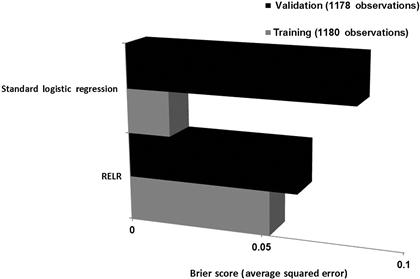
Figure 2.7 Accuracy comparison based upon Brier Score of Full RELR and Standard Logistic Regression models that have been previously reported44 based upon public domain survey data on the 2004 US Presidential Election Weekend survey that was provided by Pew Research. The identical 176 features that included interaction and nonlinear features were included in both the RELR and the Standard Logistic Regression model. Notice how RELR shows substantially less overfitting error than Standard Logistic Regression as suggested by the Brier Scores that were substantially more accurate in the Validation sample. The methods used to produce this comparison are described in detail in Appendix A1.
At its core, RELR is simply based upon the Jaynes idea that the most probable inference is the maximum entropy solution subject to all known constraints. This simple data-driven approach to evidence-based reasoning has been successfully applied to scientific inference since Boltzmann. As with standard logistic regression, RELR's constrained maximum entropy solution is identical to the maximum likelihood solution. Indeed, RELR simply generates the most likely inference when error probability constraints related to uncertainty in measurements are added to the standard logistic regression model.
Because of this ability to estimate error, RELR can model effects of higher level factors like schools or hospitals in correlated observations simply by including a dummy coded cluster indicator provided that the lowest observation level is composed of independent observations like persons. Any causal effects that exist at a higher cluster level such as related to specific schools or hospitals can be accounted for by the indicator variables, as RELR allows all levels of dummy coded indicator variables to be modeled without dropping a level to avoid multicollinearity error as must be done in standard logistic regression. This is one of the many advantages of RELR's ability to return stable regression coefficients due to its error modeling. Because of this error modeling, RELR has the ability to model uncertainty related to all measured and unmeasured constraints and return a most likely solution given that uncertainty. This goes beyond the Jaynes principle because the constraints that RELR uses to model error are not known with certainty but are instead only most likely constraints. Yet, RELR and its error modeling are still consistent with the overall Jaynes philosophy which is to arrive at a most likely inference.
In fact, RELR's explicit feature selection also can select parsimonious features that are not known with certainty in a causal sense, but are at least interpretable and consistent with causality until experimental data suggest otherwise. In addition, RELR's implicit feature selection can select a large number of features which are unlikely to be interpretable because of the complexity, but which are likely to generate a reasonable prediction provided that the predictive environment is stable. Alternatively, with a fixed set of features, RELR's sequential learning of longitudinal observations can detect the difference between a stable predictive environment versus an unstable and changing predictive environment and compute maximum probability weight changes accordingly. RELR's online learning has “memory” for previous observation episodes, which is not possible in standard logistic regression. Thus, RELR can model longitudinal data without violating independent observation assumptions. These maximum probability learning and memory abilities are reviewed in the next chapter.