
Mobile Cloud Offloading Models
A true capitalist does not have a job, because other people and other people's money work for them.
Robert Kiyosaki
Abstract
Mobile cloud offloading models are usually modeled as an application graph mapped to a surrogate network. An application is a directed acyclic graph, where vertexes are computation tasks and edges are data channels connecting tasks. The sites that run offloaded codes may be one surrogate or a network of devices. To offload the computation tasks to the surrogate network is to map the vertexes and edges from application graph to the surrogate network. In general, offloading objectives usually target saving mobile device's energy and decreasing application's execution time, and an optimal mapping may exist at a given time point. For a longer time span, a series of offloading mappings may exist to optimize an offloading objective function. In this chapter, we present a set of mobile cloud computing offloading decision models to demonstrate the mathematical construction to build one-to-one, one-to-many, and many-to-many offloading decision models. A preliminary set of evaluation results also presented to demonstrate the trade-offs of using offloading approaches with different system parameters' setup.
Keywords
Offloading mapping; One-to-one offloading; One-to-many offloading; Many-to-many offloading; Offloading objective; Surrogate; Service composition
Chapter 4 describes the mobile cloud service systems. Based on the mobile cloud system, many computation offloading strategies are developed. Yang et al. [285] studied the partitioning problem for mobile data stream applications, where the optimization focus is placed on achieving high throughput of processing the streaming data rather than minimizing the makespan (i.e., the total length of the schedule, that is when all the jobs have finished processing) of executions as in other applications. They designed a genetic algorithm for optimal computation partition. Abebe et al. [47] proposed a type of adaptation granularity which combines the efficiency of coarse level approaches with the efficacy of fine-grained adaptation. An approach for achieving this level of granularity through the dynamic decomposition of runtime class graphs was presented. Abebe et al. [48] presented a distributed approach to application representation in which each device maintains a graph consisting only of components in its memory space, while maintaining abstraction elements for components in remote devices. An extension to an existing application graph partitioning heuristic is proposed to utilize this representation approach. Giurgiu et al. [116] developed a system that dynamically adapts the application partition decisions. The system works by continuously profiling an applications performance and dynamically updating its distributed deployment to accommodate changes in the network bandwidth, devices CPU utilization, and data loads. Sinha et al. [249] and Mtibaa et al. [208] described algorithmic approaches for performing fine-grained, multisite offloading. This allows portions of an application to be offloaded in a data-centric manner, even if that data exists at multiple sites. Kovachev [170] presented Mobile Augmentation Cloud Services (MACS) middleware which enables adaptive extension of Android application execution from a mobile client into the cloud. MACS uses a dynamic partitioning scheme, and lightweight as extra profiling. Resource monitoring is performed for adaptive partitioning decision during runtime. Ra et al. [231] experimentally and analytically investigated the design considerations – which segments of the application are most efficient to be hosted on the low power processor, and how to select an appropriate low power processor using linear programming. Smit et al. [250] described an approach to partitioning a software application into components that can be run in the public cloud and components that should remain in the private data center. Static code analysis was used to automatically establish a partitioning based on low-effort input from the developer. Niu et al. [217] took the bandwidth as a variable to improve static partitioning and avoid high costs of dynamic partitioning. They proposed the Branch-and-Bound based Application Partitioning (BBAP) algorithm and Min-Cut based Greedy Application Partitioning (MCGAP) algorithm based on application Object Relation Graphs (ORGs) by combining static analysis and dynamic profiling. Verbelen et al. [266] designed graph partitioning algorithms that allocate software components to machines in the cloud while minimizing the required bandwidth. Their algorithms are not restricted to balanced partitions and take into account infrastructure heterogeneity. Besides the above work, [72][75][85][114][131][209][243][244] discussed the mobile cloud systems in specific areas.
This chapter first describes the general mobile cloud offloading setup in Section 5.1, then presents the offloading models including one-to-one case in Section 5.2 and many-to-many case in Section 5.3. Section 5.4 finally discusses the research challenges.
5.1 Mobile Cloud Offloading Setup
In mobile clouds, mobile devices and cloud resources compose a distributed mobile application running environment, where a mobile application may consume resources from both local and remote resource providers who provide computing, networking, sensing, and storage resource provisioning. Mobile devices can serve as either service consumers or service providers in the mobile cloud, in which the cloud boundaries are extended into the mobile domain [140]. Mobile applications may require a mobile device to interact with other mobile devices and cloud resource providers to achieve desired computing, storing, collaborating, or sensing features.
An ideal mobile cloud application running system should enable mobile devices to easily discover and compose cloud resources for its applications. From mobile resource providers' perspective, they may not even know what applications are using their resources and who may call their provisioned functions beforehand. In this way, the mobile application design should not be application-oriented; instead, it should be functionality-oriented (or service-oriented). For example, the video function of a mobile device should provide general interfaces that can be called by multiple local or remote functions in the runtime. To achieve this feature, we can consider these PFs as the fundamental application components in the mobile cloud, which can be composed by mobile cloud service requesters in the runtime. As a result, mobile cloud can significantly reduce the mobile application development overhead and greatly improve the agility and flexibility to build a personalized mobile cloud computing system that can be customized for each mobile user.
A simple vehicular video sensing example is used to illustrate the above described mobile cloud features. Alice is driving on the road and her smart phone, which is mounted on the front dashboard for navigation, has the basic video capture PF. Bob is driving next to Alice and is running an image processing PF on his phone and wants to utilize more video clips from the neighboring vehicles in order to reconstruct the road situations around his vicinity. Then, Bob can consume Alice's video PF to reconstruct the view of the entire road segment captured by their video cameras. Moreover, Bob wants to share his captured video clips to his friend Carol who is managing a traffic monitoring website that posts videos from smart phone users for the public to access the real-time road traffic information. As a result, Bob can share his augmented traffic view with Alice, i.e., through Carol's website. In this mobile application scenario, all participants have the basic PFs: (a) Alice, video capture; (b) Bob, video augmentation; and (c) Carol, video display. Note that a PF can be called by multiple other PFs for different application purposes, and they altogether can build several mobile cloud applications.
There are several challenges invoked by the application scenario described above. The first challenge is that knowing the status of mobile devices, e.g., online/offline and runtime information (such as battery, computing power, connectivity, etc.), is difficult due to the mobility of mobile users. The second challenge is that knowing the available PFs on each mobile device is not a trivial task. Currently, there is no such common framework allowing mobile devices for exchanging the available PFs information and running such a system in a distributed environment. The third challenge is to compose PFs crossing various hardware and software platforms, which demands a universal programming and application running environment with little compatibility issues.
5.1.1 Application-Surrogate Offloading Mapping
The mobile cloud offloading solves the partition problem to map the application components to the surrogate sites. The modular mobile applications are composed by a group of small components between which the data exchange happens. Some of the application components that can be moved to other places to run are the offloading subjects. The devices or the machines that can host these movable application components are surrogates. The offloading partition problem maps the application components to the surrogate sites as shown in Fig. 5.1.

The offloading mapping or the offloading topology decides code or task space distribution. Moreover, the offloading topology can change for the long time horizon. Based on the space and time attributes, we can categorize the mobile cloud offloading problem into 8 types as shown in Fig. 5.2. We will discuss the most simple category in Section 5.2 and the most complex category in Section 5.3. This section discusses the general offloading topology and offloading series.

Offloading Topology
Application components and the surrogate sites are the two sides of the offloading topology. While there can be one or multiple application components and there can be one or multiple surrogate sites, there are four total combinations. They are ![]() ,
, ![]() ,
, ![]() , and
, and ![]() topologies.
topologies.
If a Boolean matrix named E is used to describe the mapping and the rows corresponding to application components and the columns are corresponding to surrogate sites, the four topologies are ![]() ,
, ![]() ,
, ![]() , and
, and ![]() . For each row, there are at least one 1 since that application component has to find a surrogate to run. If there is more than one surrogate running an application component, that application component gets duplicate copies to be resistant to device or network failures.
. For each row, there are at least one 1 since that application component has to find a surrogate to run. If there is more than one surrogate running an application component, that application component gets duplicate copies to be resistant to device or network failures.
Offloading Series
The execution environment changes with time, thus the impact of one time offloading may diminish. In this scenario, the subsequent offloading may be applied to adjust the offloading topology and maintain the offloading benefit. Multiple offloading forms the offloading series. For each offloading topology above, there could be a series as shown in Fig. 5.2.
5.1.2 Offloading Objectives
In our framework, a mobile application is programmed based on component-based design, where components provide functionality via interfaces and may, conversely, consume functionality provided by other components via their interfaces [125]. The application can be presented as a graph ![]() where each vertex is a component
where each vertex is a component ![]() and an edge
and an edge ![]() represents the interaction between components [275].
represents the interaction between components [275].
In a multisite offloading scenario, some computation workload is offloaded from an original mobile device and distributed onto candidate surrogate sites. The original site and its candidate surrogate sites form an egocentric network ![]() , where a node is a site
, where a node is a site ![]() and a link
and a link ![]() represents a network connection between two sites.
represents a network connection between two sites.
The multisite offloading problem can be modeled to find a mapping from the application graph ![]() to the candidate network
to the candidate network ![]() to achieve a given optimization objective function. Let matrix E present this mapping, whose element
to achieve a given optimization objective function. Let matrix E present this mapping, whose element ![]() is set to either 1 when component i is assigned to site j or 0 otherwise. Matrix E has the following properties:
is set to either 1 when component i is assigned to site j or 0 otherwise. Matrix E has the following properties:
1. Let n be the order of all components ![]() and m be the order of all candidate sites
and m be the order of all candidate sites ![]() . Therefore, E is a matrix
. Therefore, E is a matrix ![]() . The relation of n and m is not strict, thus
. The relation of n and m is not strict, thus ![]() ,
, ![]() , and
, and ![]() are all valid.
are all valid.
2. Each component in the offloading application is assigned to exact one site, which means there is one and only one 1 in each row of E. As a result, ![]() for every row i.
for every row i.
3. In a mobile application, some components must be assigned to particular sites due to application requirements. For example, the human–machine interaction component must be put on the local mobile site. This requirement enforces that positions of some 1's in E are predefined and cannot be moved.
Based on E, four more mappings can be defined. Mapping ![]() implements a similar function as E, which maps component i to site j:
implements a similar function as E, which maps component i to site j: ![]() ,
, ![]() ,
, ![]() . Mapping
. Mapping ![]() is the reverse mapping of
is the reverse mapping of ![]() , which given site j outputs a set of components
, which given site j outputs a set of components ![]() coded as a vector i. Besides, mappings can also be defined between W and U. Mapping
coded as a vector i. Besides, mappings can also be defined between W and U. Mapping ![]() maps edge
maps edge ![]() to link
to link ![]() ; and similar to
; and similar to ![]() ,
, ![]() maps a link to a vector of edges. These four mappings can easily be expended to accept vectors as well.
maps a link to a vector of edges. These four mappings can easily be expended to accept vectors as well.
Execution Time
According to [269], at any time, the computation load for every component and the volume of data exchange for every edge in application graph is known based on a given task, or is predictable based on the application and user historical behavior. The workload is distributed on the application graph, which makes ![]() into a weighted graph. The computation load is presented as a weight value on each vertex: the component x is labeled with computation load
into a weighted graph. The computation load is presented as a weight value on each vertex: the component x is labeled with computation load ![]() and vector w is computation load of all vertexes. The data exchange amount is presented as a weight value on an edge: the edge
and vector w is computation load of all vertexes. The data exchange amount is presented as a weight value on an edge: the edge ![]() from
from ![]() to
to ![]() is labeled with data transfer load
is labeled with data transfer load ![]() and matrix
and matrix ![]() is data exchange load of all edges. The diagonal of F are all 0's because the component's interaction with itself does not count for intercomponent data exchange load; and
is data exchange load of all edges. The diagonal of F are all 0's because the component's interaction with itself does not count for intercomponent data exchange load; and ![]() if
if ![]() is false.
is false.
Meanwhile, the surrogates' capability is measurable, so the egocentric network ![]() is transformed into a weighted graph as well. The available computation capability on a candidate site s is labeled as a vertex weight
is transformed into a weighted graph as well. The available computation capability on a candidate site s is labeled as a vertex weight ![]() and vector u is the weights of all the sites. The network throughput on link
and vector u is the weights of all the sites. The network throughput on link ![]() from
from ![]() to
to ![]() is labeled as link weight
is labeled as link weight ![]() and matrix
and matrix ![]() is the weights of all the links. The diagonal of D are large values because data exchange in the same site can be considered negligible.
is the weights of all the links. The diagonal of D are large values because data exchange in the same site can be considered negligible.
In this article, we define the operator .⁎ as array inner multiplication that multiplies arrays or matrices in an element-by-element way, which is different from matrix multiplication. Let ![]() be the vector that satisfies
be the vector that satisfies ![]() where 1 is the vector whose elements are all 1's. Then the upper bound of total time spent for computation load is the sum of workload on every site over its processing capability:
where 1 is the vector whose elements are all 1's. Then the upper bound of total time spent for computation load is the sum of workload on every site over its processing capability:
Similarly, let ![]() be the matrix that satisfies
be the matrix that satisfies ![]() where
where ![]() is the matrix whose elements are all 1's. The transformation
is the matrix whose elements are all 1's. The transformation ![]() redistributes the communication load of
redistributes the communication load of ![]() into an
into an ![]() matrix where element positions are corresponding to
matrix where element positions are corresponding to ![]() . The upper bound of total time spent on networks for data exchange load is the sum of workload on every link over its throughput:
. The upper bound of total time spent on networks for data exchange load is the sum of workload on every link over its throughput:
where the ![]() function calculates matrix trace
function calculates matrix trace ![]() . So the upper bound of total time is the sum of the computation and communication times:
. So the upper bound of total time is the sum of the computation and communication times:
Energy Consumption
Energy consumption on mobile devices can be categorized according to hardware modules. The major categories are CPU, radio module (including WiFi and Cellular), display, audio device, GPS module, and vibration motor [153][245][286][289]. The components that involve modules, except CPU and radio, are hardware dependent components that have to run on the original mobile device and are not considered for offloading. Both CPU and radio power can be modeled as a linear model that consists of two parts: base consumption and dynamic consumption when hardware module is active [196][269]. The dynamic part of CPU power is proportional to the utilized processing capability according to [153][206][245][289]:
where ![]() is the coefficient vector for all sites, and the coefficients of nonmobile sites in
is the coefficient vector for all sites, and the coefficients of nonmobile sites in ![]() are 0's. Let's code E as e, then the dynamic part of radio module power is proportional to the outgoing packet rate [153][289]:
are 0's. Let's code E as e, then the dynamic part of radio module power is proportional to the outgoing packet rate [153][289]:

where ![]() is the coefficient vector for all sites, I is the identity matrix, and
is the coefficient vector for all sites, I is the identity matrix, and ![]() is the element of
is the element of ![]() corresponding to link l. The coefficients of nonmobile sites in
corresponding to link l. The coefficients of nonmobile sites in ![]() are 0's. Let
are 0's. Let ![]() be the static part of CPU power and
be the static part of CPU power and ![]() be the static power of radio module. Then the total power is the sum of the above four parts:
be the static power of radio module. Then the total power is the sum of the above four parts:
5.2 One-to-One Offloading Case
A mobile cloud consists of mobile devices and cloud. There is usually one-to-one mapping between mobile devices and virtual machines in the cloud [138]. A mobile cloud application is constructed as a set of components or bundles. Some components can run on either mobile devices or virtual machines, while the other components, such as user interface and sensors, have to run on mobile devices. The major offloading objectives are saving application execution time and energy consumption on mobile devices. Notation in the following discussion is summarized in Table 5.1 for convenience.
Table 5.1
Notation
| Terms | Meaning | Terms | Meaning |
| B | bundle set | b i | a bundle |
| e ij | service dependency from |
Bphone, Bcloud | bundle set for smart phone and cloud separately |
| t i | execution time of bi | c | partition configuration |
| t phone | application execution time in non-offloading mode | p(c) | offloading rate |
| q | how faster cloud is than smart phone | d ij | size of data transferred over |
| w | bandwidth | t(c) | total execution time |
| t′(c) | total execution time in unstable network | ξ, η | on state duration, off state duration |
| χ | cycle duration, χ = ξ + η | ρ | network availability, ρ = ξ/χ |
| PCPU(c), PRF(c) | energy consumption for CPU and RF separately | energy consumption in unstable network | |
| P(c) | total energy consumption on mobile device | P′(c) | total energy consumption in unstable network |
| P phone | energy consumption in nonoffloading mode | critical value for time and energy benefit | |
| ρ′(c) | circuital value for both time and energy benefit | Δt(c), ΔP(c) | time benefit, energy benefit |
| power of CPU and RF on smart phone |

5.2.1 Application Model and Ideal Network Model
The application is presented as a directed acyclic graph ![]() where every vertex is a bundle and every edge is the data exchange between bundles [117]. Each bundle has an attribute indicating whether it can be offloaded. The unmovable bundles are marked as local, which means these bundles cannot be offloaded due to application requirements. Let
where every vertex is a bundle and every edge is the data exchange between bundles [117]. Each bundle has an attribute indicating whether it can be offloaded. The unmovable bundles are marked as local, which means these bundles cannot be offloaded due to application requirements. Let ![]() be the total count of bundles in the application, then the initial bundle set is
be the total count of bundles in the application, then the initial bundle set is ![]() and the edge set is
and the edge set is ![]() where
where ![]() represents directed data transfer from
represents directed data transfer from ![]() to
to ![]() . Let n be the count of movable bundles and
. Let n be the count of movable bundles and ![]() . A configuration c [117] is defined as a tuple of partitions from the initial bundle set,
. A configuration c [117] is defined as a tuple of partitions from the initial bundle set, ![]() , where
, where ![]() has k bundles and
has k bundles and ![]() has s bundles. And they satisfy
has s bundles. And they satisfy ![]() and
and ![]() . The bundles that are marked as local are initially put in the set
. The bundles that are marked as local are initially put in the set ![]() and cannot be moved. An example is shown in Fig. 5.3 where unmovable bundles are marked as gray and dotted line indicates configuration. The bundles on the left side are
and cannot be moved. An example is shown in Fig. 5.3 where unmovable bundles are marked as gray and dotted line indicates configuration. The bundles on the left side are ![]() and the bundles on the right side are
and the bundles on the right side are ![]() .
.

Execution Time
For a given task, bundle ![]() has an attribute
has an attribute ![]() indicating its computation time on smart phone. And edge
indicating its computation time on smart phone. And edge ![]() is associated with an attribute
is associated with an attribute ![]() indicating the transferred date size from bundle i to bundle j. These values can be measured or estimated from collected application and device data. Total time of running the task only on the smart phone is
indicating the transferred date size from bundle i to bundle j. These values can be measured or estimated from collected application and device data. Total time of running the task only on the smart phone is

where data exchanges between bundles are not counted as they happen locally and cost little time compared to time of data exchange over the network. For a particular configuration c, offloading rate p [224] is defined as the proportion of offloaded task to all tasks in terms of computation time. The proportion of the task is the same as time proportion due to the same processing capability on the same mobile device ![]() , and
, and ![]() satisfies
satisfies ![]() . Then, the computation time on the smart phone is
. Then, the computation time on the smart phone is

Assume the cloud is q times faster than the smart phone, thus the time consumption in the cloud is q times less than the time spent on the mobile device [281], which is ![]() . The computation time in the cloud is
. The computation time in the cloud is

Thus the total computation time is

A typical offloading process works as follows: Initially, the application starts on the smart phone and all components run locally. Then, the application may offload some components to a remote virtual machine. These offloaded bundles run in the cloud remotely. However, they need to communicate with the bundles resident on the smart phone. Thus, they have to exchange data through the network. Assume that the network bandwidth is w, then the network delay is the sum of delays in both data transfer directions, namely

In an ideal network environment, the total execution time for a given configuration c is the sum of computation time and network delay, that is,
The offloading benefit of execution time comes from the trade of ![]() and
and ![]() . The computation part saves execution time because the cloud processing capability is greater than that of the mobile device. However, the offloading has to pay for network delay, which counteracts the computation time saving. For computation-intensive applications whose computation time saving is much larger than the network delay, the offloading benefit is obviously seen.
. The computation part saves execution time because the cloud processing capability is greater than that of the mobile device. However, the offloading has to pay for network delay, which counteracts the computation time saving. For computation-intensive applications whose computation time saving is much larger than the network delay, the offloading benefit is obviously seen.
Energy Consumption
Two hardware modules of the mobile device are involved in the energy consumption estimation: CPU and radio frequency (RF) module. Other modules like display, audio, GPS etc., are not considered because the components that interact with these modules have to run on the mobile device locally. The energy consumption on both CPU and RF modules can be further separated into the dynamic and static parts [269]. When the hardware module is in the idle state, the energy consumption is corresponding to the static part. When the hardware module is in the active state, more energy is consumed, which is corresponding to the dynamic part. Assume that the power of CPU in the idle state is ![]() and the power of CPU in the active state is
and the power of CPU in the active state is ![]() . The energy consumption of CPU is then
. The energy consumption of CPU is then
Similarly, let ![]() and
and ![]() be the power of RF module in the idle and active states separately. The energy consumption on radio frequency module is
be the power of RF module in the idle and active states separately. The energy consumption on radio frequency module is
Thus, the total energy consumption is
If offloading is not applied, only CPU consumes energy and its active period is the whole execution time. The total energy consumption of running tasks only on the smart phone is
The offloading influences energy consumption of the mobile device in two aspects. First, the mobile device may save energy because the mobile device does not pay for the energy consumption corresponding to the tasks that are offloaded and completed in the cloud. Second, the data exchanges between application components are now fulfilled by networking instead of local procedure invocation, which leads to energy cost for sending and receiving packets. Similar to the time benefit of offloading, the computation-intensive application may obtain an obvious energy benefit when computation tasks are offloaded as large CPU energy consumption is spared and network energy consumption is small.
5.2.2 Model and Impact of Network Unavailability
Connection between the mobile device and the cloud is usually not stable due to mobility of devices. When the mobile device moves out of wireless coverage, it loses connection to the cloud. The mobile device continues to make attempts to reconnect to the cloud when the network is unavailable. When it moves into coverage again, the connection resumes. As the mobile device moves, the connection state changes as on, off, on, off, …, which can be modeled as an alternating renewal process.
Fig. 5.4 shows how network availability changes along with time. The solid line represents that the network is available, while the dashed line represents that the network is unavailable. Two network states alternate with each other. One on duration and one off duration form a cycle. The on state duration is denoted as ξ and the off state duration is denoted as η. The variables ![]() are independent and identically distributed (i.i.d.), and so are
are independent and identically distributed (i.i.d.), and so are ![]() . And
. And ![]() and
and ![]() are independent for any
are independent for any ![]() , but
, but ![]() and
and ![]() can be dependent [228]. The cycle duration is denoted as χ, and
can be dependent [228]. The cycle duration is denoted as χ, and ![]() where
where ![]() . The proportion of on duration in any individual cycle is a random variable denoted as
. The proportion of on duration in any individual cycle is a random variable denoted as ![]() .
.

Execution Time
When the network is unavailable, the application has to wait because the phone cannot send input to the cloud and cannot retrieve output from the cloud either. The application resumes the execution after the network becomes available again. The total execution time is prolonged according to the proportion of ρ, namely

The offloading gives time benefit when ![]() . In an ideal network environment,
. In an ideal network environment, ![]() and
and ![]() .
. ![]() rises to infinity when ρ decreases from 1 to 0. At some point, the benefit finally disappears. We define this point as a critical value of ρ for the time benefit,
rises to infinity when ρ decreases from 1 to 0. At some point, the benefit finally disappears. We define this point as a critical value of ρ for the time benefit,

And the time benefit is
when ![]() .
.
Energy Consumption
During the time ![]() , the computation time
, the computation time ![]() and network time
and network time ![]() are the same as
are the same as ![]() and
and ![]() , respectively, in an ideal network environment because computation and data transfer only work properly when an ideal network is available. The CPU active time period is the same as that in an ideal network model because the given task is the same. However, the CPU idle time period is the whole execution time that is different from that in an ideal network model. Thus, the energy consumption for CPU is
, respectively, in an ideal network environment because computation and data transfer only work properly when an ideal network is available. The CPU active time period is the same as that in an ideal network model because the given task is the same. However, the CPU idle time period is the whole execution time that is different from that in an ideal network model. Thus, the energy consumption for CPU is
The RF module is active even when the network is unavailable because it continues scanning for the available network to resume connection. Thus, the active time period for the RF module is ![]() . The energy consumption for RF is
. The energy consumption for RF is
Thus, the total energy consumption is
The offloading gives energy benefit if ![]() . As ρ decreases, both
. As ρ decreases, both ![]() and
and ![]() increase. Similarly, the critical value of ρ for energy is defined as the point where the energy benefit disappears, i.e.,
increase. Similarly, the critical value of ρ for energy is defined as the point where the energy benefit disappears, i.e.,

And the offloading energy benefit is
when ![]() .
.
Problem Formulation
When network availability ρ is greater than the larger of the ![]() and
and ![]() , both time and energy benefits are obtained. We define the critical value of ρ as
, both time and energy benefits are obtained. We define the critical value of ρ as
The offloading problem with possible network unavailability is finding the application partition c to minimize ![]() :
:
while both time and energy benefits exist, i.e., when
where ρ is the current network availability estimated based on observations. The c satisfying (5.28) may not exist when ρ is too low. In this situation, the application should not offload any components to the cloud. The solution to (5.27) is the best partition that tolerates network unavailability, and it may give benefit when current network availability ρ gets worse.
5.2.3 Optimization Solution and Simulation Analysis
Bundle computation times ![]() form a vector t of dimension m. Data sizes
form a vector t of dimension m. Data sizes ![]() form a square matrix
form a square matrix ![]() . If there is no edge from
. If there is no edge from ![]() to
to ![]() , then
, then ![]() is set to 0.
is set to 0.
The configuration c can be represented as a vector x of dimension m where ![]() indicates whether
indicates whether ![]() should be offloaded.
should be offloaded. ![]() means that
means that ![]() should be offloaded to a remote cloud, and
should be offloaded to a remote cloud, and ![]() =0 means
=0 means ![]() should be kept on the smart phone locally. For
should be kept on the smart phone locally. For ![]() that cannot be offloaded,
that cannot be offloaded, ![]() is set to 0 initially and does not change. Vector x has m elements in which n elements are variables and the others are 0. For simplicity, all 0s are put at the end of x.
is set to 0 initially and does not change. Vector x has m elements in which n elements are variables and the others are 0. For simplicity, all 0s are put at the end of x.
Let 1 be a column vector whose elements are all 1s, then ![]() . Offloading rate
. Offloading rate ![]() is now
is now ![]() . And
. And ![]() is
is ![]() . Thus
. Thus ![]() is finally a function of x, which is
is finally a function of x, which is ![]() .
.
The objective of the offloading decision is to find a configuration x satisfying (5.27). This is a 0–1 Integer Programming (IP) problem.
Optimization Solution
The solution space for configuration x is ![]() , which means it costs a lot of time to search for the optimal solution. To find a proper x within acceptable time, we propose an Artificial Bee Colony (ABC) [157] based algorithm. The colony consists of three types of bees: employed bees, onlooker bees, and scout bees. A bee that goes to a food source visited by it before is named an employed bee. A bee that waits in the dance area to make a selection of the food source is called an onlooker bee. And a bee that carries a random search to discover a new food source is named a scout bee. The food source is a possible solution x, and every bee can memorize one food source. It is assumed that there is only one employed bee for each food source. The memory of employed bees is considered as the consensus of the whole colony, and the food sources found by onlooker or scout bees merge into employed bees' memory in the algorithm. Assume that the number of employed bees is N and the number of onlooker bees is M
, which means it costs a lot of time to search for the optimal solution. To find a proper x within acceptable time, we propose an Artificial Bee Colony (ABC) [157] based algorithm. The colony consists of three types of bees: employed bees, onlooker bees, and scout bees. A bee that goes to a food source visited by it before is named an employed bee. A bee that waits in the dance area to make a selection of the food source is called an onlooker bee. And a bee that carries a random search to discover a new food source is named a scout bee. The food source is a possible solution x, and every bee can memorize one food source. It is assumed that there is only one employed bee for each food source. The memory of employed bees is considered as the consensus of the whole colony, and the food sources found by onlooker or scout bees merge into employed bees' memory in the algorithm. Assume that the number of employed bees is N and the number of onlooker bees is M ![]() . And let MCN be the Maximum Cycle Number. The algorithm overview is shown in Algorithm 5.1.
. And let MCN be the Maximum Cycle Number. The algorithm overview is shown in Algorithm 5.1.

In the first step, the algorithm generates a random initial population X ![]() of N solutions where the population size is the same as the number of employed bees. Based on this initial generation, the algorithm starts to evolve the generation in cycles. The evolution repeats until the cycle number reaches the limit MCN. The algorithm outputs the best solution, denoted as
of N solutions where the population size is the same as the number of employed bees. Based on this initial generation, the algorithm starts to evolve the generation in cycles. The evolution repeats until the cycle number reaches the limit MCN. The algorithm outputs the best solution, denoted as ![]() , ever found in all cycles.
, ever found in all cycles.
In the cycle, three types of bees work in sequence. The details of various bees' actions are shown in Algorithm 5.2. Employed bees produce new solutions by two local search methods:
Flip when an employed bee randomly flips one element in the vector x.
Swap when an employed bee randomly flips two elements of different values in the vector x, which is equivalent to swapping two different elements in that vector.
Each employed bee evaluates the fitness of its original solution x, newly found ![]() , and
, and ![]() by (5.26). Then, each employed bee memorizes the best one of these three food sources and forgets the others.
by (5.26). Then, each employed bee memorizes the best one of these three food sources and forgets the others.

Onlooker bees watch employed bees dancing, and plan the preferred food source. Onlooker bees record critical values of all food sources and calculate the probability for the ![]() food source as follows:
food source as follows:

Intentionally, the lower the food source's critical value, the more likely the onlooker bee would like to go. The onlooker bees choose the food source y randomly according to its probability. Since ![]() , several onlooker bees may follow the same employed bee and choose the same food source. Then each onlooker bee applies the same local search methods used by employed bees previously to explore new neighbor solutions, and picks the best one of the three. After all onlooker bees update their solution, each employed bee compares its solution with its followers' solutions, and picks the best one as its new solution.
, several onlooker bees may follow the same employed bee and choose the same food source. Then each onlooker bee applies the same local search methods used by employed bees previously to explore new neighbor solutions, and picks the best one of the three. After all onlooker bees update their solution, each employed bee compares its solution with its followers' solutions, and picks the best one as its new solution.
In our algorithm, only one scout bee is used. This scout bee randomly generates a vector z and compares z to the worst solution of employed bees. If this randomly generated z is better than the worst solution of employed bees, the corresponding employed bee memorizes this new solution and forgets the old one.
Evaluation and Tuning
In this section, we evaluate ABC based partition algorithm, including algorithm tuning and impact of different mobile applications and the cloud. We evaluate our model and algorithms in MATLAB.
We generate 200 random application graphs as a base evaluation data set. The default parameter settings are shown in Table 5.2. We use a set of typical energy parameters K for a phone according to [269]. The cloud–phone processing ability ratio q varies in a large range from previous work [274][281]. We pick a medium value from the possible range as the default value and evaluate its impact to algorithm in Section 5.2.3. We evaluate the algorithm based on three aspects: bee colony, different applications, and cloud–phone relation.
Table 5.2
Default parameter setting
| Parameter | Default value | |
| Application | m | 10 |
| n | 8 | |
| Cloud [274][281] | q | 30 |
| Phone [269] |
|
2.5 |
|
|
5 | |
|
|
1.25 | |
|
|
1.25 | |
| Algorithm | N | 3 |
| M | 5 | |

Bee Colony and Algorithm Tuning
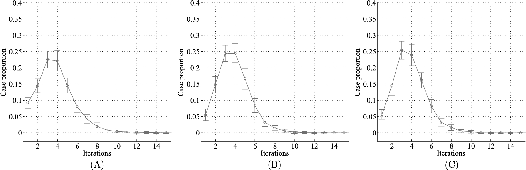
This experiment is based on 200 random application graphs (t and D). These application graphs are randomly generated, and at least one configuration of each graph is guaranteed to obtain both time and energy benefit in an ideal network environment. We evaluate the proposed algorithm performance with respect to different bee colony size. The results are shown in Fig. 5.5. The x-axis represents how many iterations the algorithm needs to reach ![]() , and the y-axis represents how many cases are needed to reach the solution of corresponding iterations. From the figure, we may draw the following guidelines for algorithm tuning:
, and the y-axis represents how many cases are needed to reach the solution of corresponding iterations. From the figure, we may draw the following guidelines for algorithm tuning:
• By increasing the onlooker bee number, the algorithm shows better convergence rate. For the same employed bee number (N), the more onlooker bees there are, the fewer iterations are obviously required to reach the optimal solution in all three situations (![]() ).
).
• While increasing the employed bee number improves convergence rate, the improvement is not as obvious compared to increasing the onlooker bee number. For the same onlooker bees of ![]() (Fig. 5.5B, Fig. 5.5D),
(Fig. 5.5B, Fig. 5.5D), ![]() (Fig. 5.5C, Fig. 5.5G), and
(Fig. 5.5C, Fig. 5.5G), and ![]() (Fig. 5.5F, Fig. 5.5H), the cases that have more employed bees have slightly better performance improvement, which is not as obvious as the improvement given by increasing onlooker bees. For
(Fig. 5.5F, Fig. 5.5H), the cases that have more employed bees have slightly better performance improvement, which is not as obvious as the improvement given by increasing onlooker bees. For ![]() figures, more than 0.05 cases reach the optimal solution in 7 iterations in Fig. 5.5C while there are only 0.05 cases that reach a solution in 7 iterations, which means more cases reach a solution in less than 7 iterations, in Fig. 5.5G. Similar phenomenon is found for
figures, more than 0.05 cases reach the optimal solution in 7 iterations in Fig. 5.5C while there are only 0.05 cases that reach a solution in 7 iterations, which means more cases reach a solution in less than 7 iterations, in Fig. 5.5G. Similar phenomenon is found for ![]() and
and ![]() figures.
figures.
• For the same total numbers of employed and onlooker bees, the algorithm prefers more onlooker bees slightly. For the same total bees of ![]() (Fig. 5.5C, Fig. 5.5D) and
(Fig. 5.5C, Fig. 5.5D) and ![]() (Fig. 5.5E, Fig. 5.5G), we can see that the overall performance is almost the same. But the iterations needed to get optimal solutions in the cases that have more onlooker bees are slightly concentrated on some iteration numbers. For
(Fig. 5.5E, Fig. 5.5G), we can see that the overall performance is almost the same. But the iterations needed to get optimal solutions in the cases that have more onlooker bees are slightly concentrated on some iteration numbers. For ![]() , the iterations in Fig. 5.5C are concentrated demonstrated by a higher summit at iteration 4, while they are diversely distributed from 1 to 8 in Fig. 5.5D. A similar situation occurs for
, the iterations in Fig. 5.5C are concentrated demonstrated by a higher summit at iteration 4, while they are diversely distributed from 1 to 8 in Fig. 5.5D. A similar situation occurs for ![]() .
.

Application Impact
To evaluate the algorithm performance for different applications, three experiments are done for varying component number, unmovable component proportion, and computation–communication ratio separately. The experiment result for different component number is shown in Fig. 5.6. For the same bee colony, the iterations to find the solution increase along with the component number. For the large applications that have many components, the algorithm may use a large bee colony to assure small number of iterations.

We evaluate the impact of unmovable component proportion of application in the second experiment, and the result is shown in Fig. 5.7. From the figure, we find that more iterations are required to get the solution when the movable component number increases. The trend is very like that in Fig. 5.6, which implies that the unmovable component number does not play a significant role in the algorithm performance. This is because the algorithm always considers the movable components and ignores the unmovable component when generating new solutions in each cycle. The total component size increase in Fig. 5.6 leads to the increase of movable component number, which is like what this experiment does in Fig. 5.7. Besides, we also found in this experiment that a higher movable proportion results in the robust solution that can work under low network availability ![]() situations. This is because the high movable proportion provides more candidate partition options so that a more robust solution may be achieved.
situations. This is because the high movable proportion provides more candidate partition options so that a more robust solution may be achieved.

We generate another two sets of application graph data for different computation load. The data sets used in previous experiments are used as the reference data set. Then we adjust the computation task to half and double of the reference data set in the application graph generation process. The network task remains the same, thus the computation–communication ratio is adjusted to half and double in the new data sets. The experiment results for these three data sets are shown in Fig. 5.8. From the figure, we can see that the iterations, distributed at ![]() , and 6, are almost the same, which implies the computation proportion of the given task does not influence the algorithm performance. This is because the computation proportion in the task influences the time and energy benefits in the same direction. In the experiment, we also find that the computation proportion impacts the
, and 6, are almost the same, which implies the computation proportion of the given task does not influence the algorithm performance. This is because the computation proportion in the task influences the time and energy benefits in the same direction. In the experiment, we also find that the computation proportion impacts the ![]() , because a larger computation proportion leads to a larger offloading benefit and the possible solution is more resistant to network unavailability.
, because a larger computation proportion leads to a larger offloading benefit and the possible solution is more resistant to network unavailability.
Cloud Impact
We evaluate the algorithm performance under different cloud speedup ratios shown in Fig. 5.9. The figure shows that the iteration number does not depend on the cloud processing capability. The cloud processing capability influences the execution time considered in the algorithm, which is similar to the computation proportion impact. And similarly, the higher cloud processing capability results in a more robust partition configuration.

5.3 Many-to-Many Offloading Case
Nowadays, many mobile cloud applications adopt a multisite service model [189][249]. To maximize the benefits from multiple service providers, the research focuses on how to compose services that have been already implemented on multiple service providers. Here, we do not differentiate between application functions and services since our model can be applied to both. A simple example can be used to highlight the application scenario: a mobile device calls a video capturing function from multiple remote mobile devices at a congested road segment, an image processing function uses this to recognize vehicles on the road segment from the cloud, and then the requesting mobile device uses its local UI to display the road traffic with identified lanes and vehicles. Compared to the traditional approach where users upload captured videos to the cloud and the requester downloads the processed videos from the cloud, the presented application scenario does not require a presetup application scenario to each function. This approach is very flexible in terms of ad hoc application composition, and it can maximally improve the resource utilization. For example, the video capturing function of mobile devices can be shared by multiple users for different purposes, e.g., congestion monitoring, road events detection, vehicle identification and tracking, etc.
Besides the flexibility of the service/function composition using multisite service composition, it also introduces benefits in reducing execution time and energy consumption of mobile devices; however, at the same time, it brings more management issues as well. The multisite service composition paradigm involves multiple surrogate sites in the service composition process, and the application running environment changes demand a decision model in the service composition decision processes to consider the application running environment changes related to network connectivity, delay, device resource consumption, energy usage, etc. Moreover, due to the mobility, the benefits of service composition may not be consistent during the entire application execution time period. To adapt to the application running environment changes, we need to study the service reconfiguration strategy by modeling the service composition as a service-topology mapping (or reconfiguration) problem that is illustrated in Fig. 5.10. Relying on a cloud service framework, once the mobile application running environment state changes, a new service-topology reconfiguration is decided, and then the application components are redistributed to the surrogate sites through the cloud. In this way, the service composition is adaptive to gain the maximum service benefits during the entire execution time period [276].

To address the above mobile cloud service composition problem, many existing approaches (e.g., [117] [160] [274]) only focus on solving the one-time service composition topology configuration without considering a sequence of service composition due to the application running environment changes (e.g., due to the mobility of nodes). When considering multiple service composition decisions, one decision may impact other service mapping decisions at an upcoming service mapping. This demands that the topology reconfiguration decision must not only consider the current environment state but also predict future environment changes, and thus, the service-topology reconfiguration issue can be modeled as a decision process issue. To address the above described issues, we model the service composition topology reconfiguration as a five-element tuple system and we present three algorithms to solve these decision process problems for three mobile cloud application scenarios: (1) finite horizon process where the application execution time is restricted by a certain time period, (2) infinite horizon process where there is no clear boundary of the application execution time, and (3) large-state situation where the large numbers of many-to-many service mappings demand a parallel computing framework to compute the service mapping decision.
The offloading as a service and service composition in mobile cloud computing achieve three essential tasks: First, the mobile application components, which can be offloaded, are partitioned into several groups. Second, the surrogate sites are picked from candidate sites that are usually virtual machines in cloud. Third, the component groups in the first task are mapped to surrogate sites in the second task, and then computation is offloaded. The service composition is not a one-time process. Instead, the mapping in the third task should be dynamically changed to adapt to the system and environment changes, especially in mobile cloud computing where mobility adds to the environment variation.
This section first describes the normal service composition system, and then models the players in the system including mobile application and surrogate network, and finally formulates the service composition topology reconfiguration process.
5.3.1 Service Composition System
The Service composition system consists of three parts shown in Fig. 5.11, which can be emulated as human decision processes. The Monitor represents the human's eyes watching both the mobile applications and infrastructure, and notifying the Service composition topology reconfiguration about their states' changes. The Service composition topology reconfiguration is the human's brain thinking about how to put application components onto which surrogate sites. The Service composition executor represents the human's hands that enforce the component–surrogate mapping and make sure a mobile device and its surrogates work together properly. These three interdependent modules can be deployed in a cloud computation platform to provide offloading-as-a-service, which exposes http REST API for mobile applications and the infrastructure to interact with. The infrastructure registers itself to the service and pushes the state information to the Monitor. The mobile application as well registers itself to the service and receives the execution command from the Service composition executor.
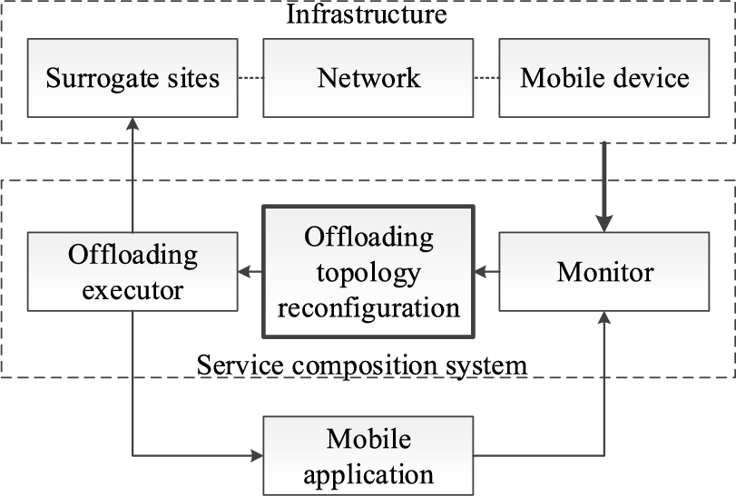
Besides the Service composition system, the Mobile application and Infrastructure are involved in the service composition process, and they form a loop where the Mobile application and the Infrastructure share a part of the loop in parallel. The Service composition system initiates the service composition operations that stimulate the Mobile application and the Infrastructure. The Mobile application and the Infrastructure integrate the service composition impacts and the variances form the outside, such as user inputs to the application and the device load variance, and feedback to the Service composition system. Then, the Service composition system based on the feedback makes the service composition operation.
The Mobile application is the objective of the Service composition system. The Infrastructure consists of the three players that are involved in the service composition process: the Mobile device, the Surrogate sites, and the Network between them; they are modeled in the following subsections.
Application Graph
A modern mobile application is usually guided by component oriented design. Components provide functionality via interfaces and may, conversely, consume functionality provided by other components [277]. The application can be presented as a graph ![]() where the vertexes are the components and the edges show the interaction between components.
where the vertexes are the components and the edges show the interaction between components.
To be extensible, the application graph is not limited to present only one application. The application graph can be extended to contain several applications and even the connections between applications.
Surrogate Network
In a multisite service composition scenario, some computation workload is offloaded from the original mobile device and distributed onto the chosen surrogate sites from candidate sites. The original site and its candidate sites form an egocentric network ![]() , where the node is the site and the link is the network connection between sites.
, where the node is the site and the link is the network connection between sites.
Component–Surrogate Mapping
The service composition mapping is a mapping from the application graph ![]() to a surrogate network
to a surrogate network ![]() , where vertexes are mapped to nodes and the edges are mapped to links correspondingly. Let matrix X present this mapping, whose element
, where vertexes are mapped to nodes and the edges are mapped to links correspondingly. Let matrix X present this mapping, whose element ![]() is set to either 1 when component i is assigned to site j or 0, otherwise. Matrix X has the following properties:
is set to either 1 when component i is assigned to site j or 0, otherwise. Matrix X has the following properties:
1. Let n be the component number, ![]() , and m be the candidate site number,
, and m be the candidate site number, ![]() . Then, E is
. Then, E is ![]() . The relation of m and n is not strict, which means
. The relation of m and n is not strict, which means ![]() ,
, ![]() , and
, and ![]() are all valid.
are all valid.
2. The mapping is also not strict, which means several components may be mapped to the same surrogate site and some surrogate site may not host any components. However, each component in the application is assigned to exactly one site, thus, there is one and only one 1 in each row of E, i.e., ![]() for every row i.
for every row i.
3. In a mobile application, some components have to be assigned to particular sites due to application requirements. For example, human–machine interaction components and sensor components have to be put on the original mobile device because they use mobile device hardware that is not available on surrogate sites. This requirement enforces the positions of some 1's in some rows of E to be predefined and not to be moved. These rows are put at the bottom of E. Except for these rows, the rest of E is the effective matrix ![]() , which corresponds to the movable components.
, which corresponds to the movable components.
Based on E, four more mappings can be defined for easy expression in the following sections. Mapping ![]() implements a similar function as E, which maps component i to site j:
implements a similar function as E, which maps component i to site j: ![]() ,
, ![]() ,
, ![]() . Mapping
. Mapping ![]() is the reverse mapping of
is the reverse mapping of ![]() , which given site j outputs a set of components
, which given site j outputs a set of components ![]() coded as a vector i. Besides, mappings can also be defined between A and B. Mapping
coded as a vector i. Besides, mappings can also be defined between A and B. Mapping ![]() maps edge
maps edge ![]() to link
to link ![]() . And similarly to
. And similarly to ![]() , mapping
, mapping ![]() maps a link to a vector of edges.
maps a link to a vector of edges.
5.3.2 Model Statement
This subsection models several factors involved in the service composition topology reconfiguration, followed by model formulation in the end.
Decision Points
Decision points are the moments when the service composition topology reconfiguration decisions are made. At these moments in Fig. 5.11, the Monitor triggers the Service composition topology reconfiguration to generate a service composition topology. The moments are decided by the Monitor that is always observing the Infrastructure and the Mobile application states. The Monitor can trigger decisions periodically according to a predefined period Δt.
The decision points are a sequence that starts from the time when the application starts to the time when the application ends, ![]() . In some scenarios, the application termination time is not expected and the sequence is an infinite sequence,
. In some scenarios, the application termination time is not expected and the sequence is an infinite sequence, ![]() .
.
Measures
The Monitor measures the Infrastructure states. The node computation capability and link throughput are labeled on the surrogate network, which transforms ![]() into a weighted graph. The available computation capability on a candidate site s is labeled as a node weight
into a weighted graph. The available computation capability on a candidate site s is labeled as a node weight ![]() and vector u collects weights of all sites. The network throughput on link
and vector u collects weights of all sites. The network throughput on link ![]() from
from ![]() to
to ![]() is labeled as link weight
is labeled as link weight ![]() and matrix
and matrix ![]() contains weights of all links. The diagonal of D has large values because the delay in the same site can be considered negligible.
contains weights of all links. The diagonal of D has large values because the delay in the same site can be considered negligible.
The above measures may be continuous variables. They are manipulated by normalization and quantization to make them into discrete states. A relatively large value is picked and the observation is scaled to be in ![]() . Quantization precision determines the size of state space. The evaluation shows the results of different state space. The state space is denoted as S.
. Quantization precision determines the size of state space. The evaluation shows the results of different state space. The state space is denoted as S.
Service Composition Topology
The service composition topology is the effective component surrogate mapping ![]() . Each mapping corresponds to an action that enforces the mapping. The size of service composition topology space is
. Each mapping corresponds to an action that enforces the mapping. The size of service composition topology space is ![]() since each component has n choices and there are
since each component has n choices and there are ![]() components that make their choices independently. Let A be the corresponding action space from which the Service composition system in Fig. 5.11 acts – picking and enforcing the mappings. The output of the Service composition topology reconfiguration is a service composition topology. If the outputted service composition topology is different from the old one, reconfiguration is needed. “Reconfiguration” means that the components in the old service composition topology should be moved properly to satisfy the new service composition topology, which is fulfilled by the Service composition executor.
components that make their choices independently. Let A be the corresponding action space from which the Service composition system in Fig. 5.11 acts – picking and enforcing the mappings. The output of the Service composition topology reconfiguration is a service composition topology. If the outputted service composition topology is different from the old one, reconfiguration is needed. “Reconfiguration” means that the components in the old service composition topology should be moved properly to satisfy the new service composition topology, which is fulfilled by the Service composition executor.
Observation Learning
The Service composition topology reconfiguration in Fig. 5.11 counts the historical states and actions, and estimates the state transition probability ![]() where
where ![]() and
and ![]() . The transition probability satisfies
. The transition probability satisfies ![]() . This probability is updated at decision points. The Service composition topology reconfiguration maintains a buffer that keeps the count for valid observed states and the count of historical actions. At each decision point, it gets the current state j from the Monitor and, the last state i and the last topology decision a from its buffer. Then it calculates the state transition probability for every pair of states with every action. This transition probability that comes from the recent history is used to predict the probability of transition for the near future Δt period assuming the transition probability stays steady in a short time period.
. This probability is updated at decision points. The Service composition topology reconfiguration maintains a buffer that keeps the count for valid observed states and the count of historical actions. At each decision point, it gets the current state j from the Monitor and, the last state i and the last topology decision a from its buffer. Then it calculates the state transition probability for every pair of states with every action. This transition probability that comes from the recent history is used to predict the probability of transition for the near future Δt period assuming the transition probability stays steady in a short time period.
Service Composition Objective
One major service composition goal in mobile cloud computing is to save mobile device energy. Following the same procedures of equations from (5.4) to (5.7), the total power is calculated through the following equations:

When a topology is picked at a decision point, a reward value is calculated to indicate how good the decision is. The reward of choosing action a at state i depends on not only state i and action a but also the next state j. The reward is

where the reward of transition from state i to state j with action a is the expected delta power between two states i and j with the same action a, and
Model Formulation
The service composition topology reconfiguration process is modeled as a five element tuple:
This is a Markov decision process [188].
5.3.3 Optimization Solution
Based on the proposed service composition topology reconfiguration system and model, this section formulates the topology reconfiguration policy problem in both finite horizon scenario and infinite horizon scenario. The solutions in both scenarios are presented. Besides, the MapReduce based algorithms are discussed for large state count situations that are common in real world.
Topology Reconfiguration Policy
The service composition reconfiguration policy is a function π that maps states to actions ![]() . The function π can be stored in memory as an array whose index is the state and whose content of each element is the corresponding action.
. The function π can be stored in memory as an array whose index is the state and whose content of each element is the corresponding action.
Let ![]() and
and ![]() be the system state and the picked action at decision point t,
be the system state and the picked action at decision point t, ![]() . The sequence
. The sequence ![]() is a stochastic process depending on π. Let
is a stochastic process depending on π. Let ![]() , then the sequence
, then the sequence ![]() is a reward process depending on π.
is a reward process depending on π.
Finite Decision Points
At any decision point, the current period reward could be used as a decision goal, which, however, is shortsighted because the maximum current period reward does not guarantee that the sum of rewards in all periods is maximum. To make a proper decision on service composition topology, the total rewards of N periods should be considered as the goal:

where β is the confidence index. As the N periods' rewards are estimated future rewards, the degree of confidence on the reward sequence ![]() decreases with t. The confidence index presents this decreasing confidence trend. The service composition topology reconfiguration problem is to find the policy π that maximizes
decreases with t. The confidence index presents this decreasing confidence trend. The service composition topology reconfiguration problem is to find the policy π that maximizes ![]() .
.
Let ![]() be the reward sum from decision point t to N. There is backward recursive relation between
be the reward sum from decision point t to N. There is backward recursive relation between ![]() and t:
and t:


where ![]() is the state at time t. Equation (5.38) shows the reward sum from time t to N consists of the current period reward and the β scaled reward sum from time
is the state at time t. Equation (5.38) shows the reward sum from time t to N consists of the current period reward and the β scaled reward sum from time ![]() to N.
to N.
Let the superscript notation ⁎ represent the maximum value of the corresponding variable. To get the maximum rewards, the backward recursive relation formulation is

Algorithm 5.3 shows the algorithm to calculate the policy π. The main body of the algorithm repeats equation (5.40) N times. In the algorithm, line 5 and line 6 could share the intermediate result of equation (5.38), which means ![]() ,
, ![]() is calculated only once but used in both operations.
is calculated only once but used in both operations.

The algorithm requires storage for two arrays indexed by state, v and f. The ith element of the array v is ![]() where
where ![]() . The ith element of the array f is an action
. The ith element of the array f is an action ![]() that is the optimal action corresponding to state
that is the optimal action corresponding to state ![]() . The array f hosts one instance of π. The length of both v and f is
. The array f hosts one instance of π. The length of both v and f is ![]() .
.
At the end of the algorithm, v contains the discounted sum of the rewards to be earned on average from the corresponding initial state i: ![]() where
where ![]() . The policy is
. The policy is ![]() for N decision points. The array f contains
for N decision points. The array f contains ![]() when the algorithm ends. The action
when the algorithm ends. The action ![]() is the action that should be performed at the current decision point.
is the action that should be performed at the current decision point.
Infinite Decision Points
The previous discussion of the finite horizon scenario can be extended to the infinite horizon scenario. The objective function for the infinite horizon scenario can be achieved by pushing N to ∞ in equation (5.37), i.e.,
Similarly, the problem is to find the policy π that maximizes the total rewards ![]() . In the infinite horizon scenario, the recursive relation (5.38) is generalized by removing iteration subscript:
. In the infinite horizon scenario, the recursive relation (5.38) is generalized by removing iteration subscript:

Similarly, the recursive relation (5.40) changes to

which means the ![]() achieves to the maximum total rewards.
achieves to the maximum total rewards.
Algorithm 5.4 shows the algorithm to calculate the policy π. Compared to Algorithm 5.3, the iteration termination condition is changed to comparing the vector norm and tolerance. ε indicates the tolerance for the converging state. In line 6, ![]() is a vector norm that could be any type of
is a vector norm that could be any type of ![]() :
: ![]() ,
, ![]() , or
, or ![]() norm. In addition, a local improvement loop is added inside the main iteration. The sequence
norm. In addition, a local improvement loop is added inside the main iteration. The sequence ![]() consists of nonnegative integers that are used in each iteration as improvement depth;
consists of nonnegative integers that are used in each iteration as improvement depth; ![]() could be generated in many ways. For example, it may be constant, i.e.,
could be generated in many ways. For example, it may be constant, i.e., ![]() , or it may get more precise along with the iteration sequence number, i.e.,
, or it may get more precise along with the iteration sequence number, i.e., ![]() . When the algorithm ends, the policy is
. When the algorithm ends, the policy is ![]() that is stored in the array f.
that is stored in the array f.

The column vector ![]() and matrix
and matrix ![]() are defined to simplify expressions in the algorithm. The ith element of vector
are defined to simplify expressions in the algorithm. The ith element of vector ![]() is
is ![]() where
where ![]() . The size of
. The size of ![]() is
is ![]() . The
. The ![]() th element of matrix
th element of matrix ![]() is
is ![]() where
where ![]() . The size of
. The size of ![]() is
is ![]() . In the algorithm, lines 13 through 15 repeat the same operations as lines 3 to 5. Line 8 is the vector version of equation (5.42). Lines 5 and 15 are the vector version of equation (5.43). Lines 3 and 5 share the intermediate computation result. Similarly, lines 13 and 15 also share the intermediate computation result.
. In the algorithm, lines 13 through 15 repeat the same operations as lines 3 to 5. Line 8 is the vector version of equation (5.42). Lines 5 and 15 are the vector version of equation (5.43). Lines 3 and 5 share the intermediate computation result. Similarly, lines 13 and 15 also share the intermediate computation result.
Large State Space
To make a more accurate and agile decision, the real world measures usually lead to a large state space in Section 5.3.2. The large state space size results in a long responding time. To mitigate the response time in a large state space situation, MapReduce could be used. This section discusses the conversion from Algorithm 5.3 and Algorithm 5.4 to MapReduce algorithms.
Algorithm 5.5 and Algorithm 5.6 show the MapReduce algorithms for the finite horizon scenario. The input to the mapper function, which is also the output of the reducer function, is the state id i and an object Q that encapsulates the state information defined in Section 5.3.2. Besides encoded state information, two components ![]() and
and ![]() corresponding to the arrays v and f are also included in the state object. Moreover, a component
corresponding to the arrays v and f are also included in the state object. Moreover, a component ![]() corresponding to the state transition probability obtained in Section 5.3.2 is included in the state object as well. The state object is passed from the mapper to the reducer for calculating Equation (5.39). This is accomplished by emitting the state data structure itself, with the state id as a key in line 2 of the mapper. In the reducer line 3, the node data structure is distinguished from other values.
corresponding to the state transition probability obtained in Section 5.3.2 is included in the state object as well. The state object is passed from the mapper to the reducer for calculating Equation (5.39). This is accomplished by emitting the state data structure itself, with the state id as a key in line 2 of the mapper. In the reducer line 3, the node data structure is distinguished from other values.


The mapper function associates the current state with all backward states. The reducer function aggregates the reward sum of all forward states according to Equation (5.39), which is categorized by action. Then it picks the maximum reward sum and the corresponding action as the current reward sum and action according to Equation (5.40).
It is apparent that Algorithm 5.3 is an iterative algorithm, where each iteration corresponds to a MapReduce job. The actual checking of the termination condition must occur outside of MapReduce. Typically, execution of an iterative MapReduce algorithm requires a non-MapReduce “driver” program, which submits a MapReduce job to iterate the algorithm, checks to see if a termination condition has been met, and if not, repeats [187].
As presented in Section 5.3.3, just as the infinite horizon algorithm is obtained by extending the finite algorithm, the MapReduce based algorithm for the infinite horizon scenario can be obtained by extending the MapReduce based finite horizon algorithms. The mapper function could be used without modification in the infinite horizon algorithms. The improvement loop in the infinite horizon algorithm can be achieved by repeating lines 8 through 12 ![]() times. Besides the modification on the reduce function, a modification on the driver is required. The iteration termination condition in the driver is changed from a fixed number to a comparison of norm and coverage tolerance.
times. Besides the modification on the reduce function, a modification on the driver is required. The iteration termination condition in the driver is changed from a fixed number to a comparison of norm and coverage tolerance.
5.3.4 Evaluation
This section discusses the proposed models and presents the evaluations of the proposed algorithms including finite horizon, infinite horizon, and MapReduce based algorithms.
Evaluation Cases and Default Parameter Setting
We generate 200 test cases of the proposed model in Section 5.3.2. To make the mobile device profile based on solid ground, we pick up the mobile device profiling parameters obtained in a previous work [289]. The maximum dynamic power consumption values in each mobile CPU and RF components, ![]() and
and ![]() , are normally distributed with mean of 4.34 and 710, and variance of 1.46 and 48, respectively. The static power consumption values in each mobile CPU and RF components,
, are normally distributed with mean of 4.34 and 710, and variance of 1.46 and 48, respectively. The static power consumption values in each mobile CPU and RF components, ![]() and
and ![]() , are normally distributed with mean of 121.46 and 20, and variance of 9.20 and 4.86, respectively. To estimate the surrogate infrastructure, we pick up the cloud profiling parameters obtained in a previous experience report [81]. The CPU utility is uniformly distributed from
, are normally distributed with mean of 121.46 and 20, and variance of 9.20 and 4.86, respectively. To estimate the surrogate infrastructure, we pick up the cloud profiling parameters obtained in a previous experience report [81]. The CPU utility is uniformly distributed from ![]() to
to ![]() . The network throughput is uniformly distributed from
. The network throughput is uniformly distributed from ![]() to
to ![]() after normalization.
after normalization.
Besides the mobile device and cloud profiling, we use the default algorithm parameter values (see Table 5.3). These values may be changed in the experiments to show their impact on the algorithms.
Table 5.3
Default parameter setting
| Parameter | Default value | |
| application and cloud |
|
8 |
| n | 5 | |
| |S| | 100 | |
| finite horizon | N | 3 |
| β | 0.7 | |
| infinite horizon | L p | L 2 |
| m n | n | |
| ε | 1 | |
| large state space | |S| | 1000 |

Experiments on Finite Horizon
We first evaluate the norm of the reward sum trend along with the variance of forecast decision point number N for different confidence index β. Since the reward sum range of test cases vary, we normalize the reward sum against the maximum reward sum in the evaluation. The experiment result is shown in Fig. 5.12. The trend in the figure shows that the reward sum approaches the maximum reward sum as N increases. The approach follows a monotonically increasing trend. When the reward sum approximates a stable value (e.g., N is greater than 8 for ![]() ), we can claim that N is large enough to be considered as an infinite horizon scenario.
), we can claim that N is large enough to be considered as an infinite horizon scenario.
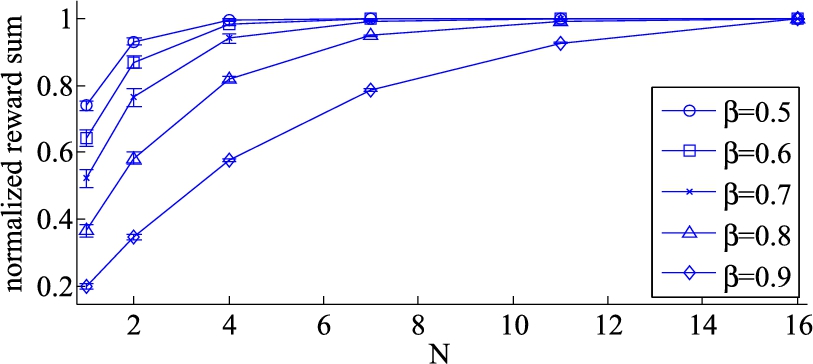
In Fig. 5.12, when the confidence index is small (![]() ), the reward sum converges after a short period (
), the reward sum converges after a short period (![]() ). When
). When ![]() , the value for the reward sum to converge (
, the value for the reward sum to converge (![]() ) is twice as that for
) is twice as that for ![]() . The higher the confidence index, the larger the decision point number to make the expected reward sum converge. Since the N values for convergence are related to the iteration times in the infinite scenario, we can infer that the smaller the confidence index, the fewer iterations are required in the infinite horizon scenario.
. The higher the confidence index, the larger the decision point number to make the expected reward sum converge. Since the N values for convergence are related to the iteration times in the infinite scenario, we can infer that the smaller the confidence index, the fewer iterations are required in the infinite horizon scenario.
We then evaluate the norm of the reward sum trend along with the variance of confidence index β. The experiment result is shown in Fig. 5.13. In the figure, the reward sum is normalized against the values of the default confidence index. The reward sum increases monotonically along with the confidence index. The higher the confidence index, the more reward values are added to the total considered reward, which leads to the higher norm value of the reward norm. The reward sum increases sharply when the confidence index approaches 1, which leads to a linear proportional relation between the reward sum and the forecast period N or an infinite horizon reward sum calculation failure. When the confidence index is small, the reward sum is steady because the reward sum mainly consists of rewards in several near future forecast periods.

Experiments on Infinite Horizon
In the infinite horizon algorithm, the main loop of the infinite horizon algorithm terminates using a condition controlled by the reward sum tolerance. We experiment with different tolerance and their corresponding main loop iteration cycles and show the results in Fig. 5.14. In the figure, the x-axis ranges from 1 times ε to 50 times ε, and the y-axis is the iteration cycle number that is normalized against the cycle number of the default ε situation. Obviously, the higher the tolerance, the sooner the iteration ends. A large tolerance means that larger reward sum values fall into the area of considered converged values, so fewer iterations may let the reward sum trend go into that area and terminate the iteration cycle. We also illustrate the reward sum of different ε in Fig. 5.15. Here, similar to Fig. 5.14, the x-axis ranges from 1 times ε to 50 times ε, and the y-axis is the reward sum that is normalized against the cycle number of the default ε situation. We can see that the reward sum decreases when the tolerance increases, which demonstrates the that the coverage area is enlarged by the large tolerance. In addition, the reward sum decreases proportionally to the tolerance variance, which is expected because the convergence area is enlarged by turbulence proportionally.


5.4 Evolving Mobile Cloud Computing
In the previous and this chapter, we saw how a mobile cloud system works. The world changes fast, as does the mobile cloud. In this section, we discuss several promising research areas of mobile cloud computing, hoping to inspire users explore future research ideas.
Semantic Compute Offloading
Information-centric networking (ICN) is initially conceptualized as a general form of communication architecture to achieve efficient content distribution on the Internet. ICN focuses on what (content) instead of where (host). This is to fulfill the primary demands that consumers are only interested in content itself, not its provenance, and publishers strive to efficiently distribute contents to consumers. To this end, ICN uses node or data attributes (e.g., content name, geo-location, or context) for routing rather than a specific node address (i.e., IP address). This decouples the content from the publishers. In this sense, content-based routing, geo-routing, and context-based routing can be classified into types of ICN [177].
Service discovery plays a key role in the computation offloading and service composition. The current mobile cloud offloading systems and strategies work based on the addresses. Thus, a system-wide central service registry or service broker is necessary to route the offloading request or to answer the service searching. When ICN is introduced to fulfill the service discovery of the mobile cloud offloading, the offloading architecture may be simplified and the service composition can be more flexible.
MicroService
A microservice [100] [179] [261] [214] is a minimal functional service module which is independently developed and deployed, and microservice architecture is an architecture of distributed software modules composed by a microservice which is rather an evolved software engineering pattern from successful field practice as opposed to an invented principle. The major characteristics of microservice include small, focused, self-contained service for componentization, loosely coupled architecture, clear boundary by contexts, autonomous and software architecture aligned development team, decentralized governance, design for failure, etc. These architectural characteristics bring many benefits such as capability of integration of heterogeneous technology, continuous delivery, resilience, scalability, and eventually a fast-evolutionary architecture.
Microservice patterns are mainly discussed in the context of large web based applications, while less focus has been on the IoT system. It is interesting to see that they actually share many similar characteristics [70] [172]. First, they have a similar loosely coupled architecture. A typical IoT system will integrate many devices and software components from different vendors, where each of them has its own life cycle. Second, most IoT systems need to integrate heterogeneous software components implemented on different hardware devices. To cope with the fast-evolving technology, some of them might be changed or updated without the influence of the other parts of the system. Third, communications among different software modules in an IoT system are usually based on well-defined message oriented interfaces, or REST API, which is similar to calling a service. Fourth, they both try to maintain minimum deployment and management effort in the field. The smaller the services, the easier it is to offload. Especially on the IOT devices, which are more resource constrained than smart phones, offloading the tasks to other devices might be necessary. Besides, the number of IOT devices may be much larger than that of phones, which leads to offloading scalability research topic.
Multistage Offloading
The present offloading model regards the mobile device and cloud as the only two layers in the model. However, more devices are involved in the mobile cloud system, such as IOT devices, vehicles, road site units, and mobile stations. These devices are equipped with computation and storage capability, which can host offloaded computation. The advantage of these devices compared to the Internet cloud is that they are closer to the user. Naturally, they can be candidate surrogates. A typical example is the vehicle cloud. When a smart phone connects to a vehicle, the computation can be offloaded from the phone to the vehicle, which is supposed to be faster than that offloaded to the Internet cloud due to network length. However, the computation and storage on the vehicle are still limited compared to the cloud. In some application scenarios, the vehicle cannot provide all the required resources and the vehicle may choose to offload the overload compute request to the road site unit or further Internet cloud. The cascading offloading for multistage offloading is more suitable in the present world where everything gets smart.