Chapter 1: Introduction to Sound

Sound is something most people take for granted. Our environment is full of noises, which we have been exposed to from before birth. What is sound, how does it propagate, and how can it be quantified? The purpose of this chapter is to introduce the reader to the basic elements of sound, the way it propagates, and related topics. This will help us to understand both the nature of sound and its behavior in a variety of acoustic contexts, and allow us to understand both the operation of musical instruments and the interaction of sound with our hearing.

1.1 Pressure Waves and Sound Transmission

At a physical level sound is simply a mechanical disturbance of the medium, which may be air, or a solid, liquid or other gas. However, such a simplistic description is not very useful as it provides no information about the way this disturbance travels, or any of its characteristics other than the requirement for a medium in order for it to propagate. What is required is a more accurate description which can be used to make predictions of the behavior of sound in a variety of contexts.

1.1.1 The Nature of Sound Waves

Consider the simple mechanical model of the propagation of sound through some physical medium, shown in Figure 1.1. This shows a simple one-dimensional model of a physical medium, such as air, which we call the golf ball and spring model because it consists of a series of masses, e.g., golf balls, connected together by springs. The golf balls represent the point masses of the molecules in a real material, and the springs represent the intermolecular forces between them. If the golf ball at the end is pushed toward the others then the spring linking it to the next golf ball will be compressed and will push at the next golf ball in the line, which will compress the next spring, and so on.

Figure 1.1 Golf ball and spring model of a sound propagating material.

Because of the mass of the golf balls there will be a time lag before they start moving from the action of the connecting springs. This means that the disturbance caused by moving the first golf ball will take some time to travel down to the other end. If the golf ball at the beginning is returned to its original position the whole process just described will happen again, except that the golf balls will be pulled rather than pushed and the connecting springs will have to expand rather than compress. At the end of all this the system will end up with the golf balls having the same average spacing that they had before they were pushed and pulled.

The region where the golf balls are pushed together is known as a “compression” whereas the region where they are pulled apart is known as a “rarefaction,” and the golf balls themselves are the propagating medium. In a real propagating medium, such as air, a disturbance would naturally consist of either a compression followed by a rarefaction or a rarefaction followed by a compression in order to allow the medium to return to its normal state. A picture of what happens is shown in Figure 1.2. Because of the way the disturbance moves—the golf balls are pushed and pulled in the direction of the disturbance’s travel—this type of propagation is known as a “longitudinal wave.” Sound waves are therefore longitudinal waves which propagate via a series of compressions and rarefactions in a medium, usually air.

Figure 1.2 Golf ball and spring model of a sound pulse propagating in a material.

1.1.2 The Velocity of Sound Waves

The speed at which a disturbance, of either kind, moves down the “string” of connected golf balls will depend on two things:

The mass of the golf balls: the mass affects the speed of disturbance propagation because a golf ball with more mass will take longer to start and stop moving. In real materials the density of the material determines the effective mass of the golf balls. A higher density gives a higher effective mass and so the propagation will travel more slowly.
The strength of the springs: the strength of the springs connecting the golf balls together will also affect the speed of disturbance propagation because a stronger spring will be able to push harder on the next golf ball and so accelerate it faster. In real materials the strength of the springs is equivalent to the elastic modulus of the material, which is also known as the “Young’s modulus” of the material. A higher elastic modulus in the material implies a stiffer spring and therefore a faster speed of disturbance propagation.

Young’s modulus is a measure of the “springiness” of a material. A high Young’s modulus means the material needs more force to compress it.

It is measured in newtons per square meter (N m⁻²).

For longitudinal waves in solids, the speed of propagation is only affected by the density and Young’s modulus of the material, and this can be simply calculated from the following equation:

where c =	the speed in meters per second (ms^–1)
ρ =	the density of the material (in kg m^–3)
and E =	the Young’s modulus of the material (in N m^–2)

A newton (N) is a measure of force.

However, although the density of a solid is independent of the direction of propagation in a solid, the Young’s modulus may not be. For example, brass will have a Young’s modulus which is independent of direction because it is homogeneous, whereas wood will have a different Young’s modulus depending on whether it is measured across the grain or with the grain. Thus brass will propagate a disturbance with a velocity which is independent of direction, but in wood the velocity will depend on whether the disturbance is traveling with the grain or across it. To make this clearer let us consider an example.

c is the accepted symbol for velocity, yes it’s strange, but v is used for other things by physicists. Density is the mass per unit volume. It is measured in kilograms per cubic meter (kg m⁻³).

This variation of the speed of sound in materials such as wood can affect the acoustics of musical instruments made of wood and has particular implications for the design of loudspeaker cabinets, which are often made of wood. In general, loudspeaker manufacturers choose processed woods, such as plywood or MDF (medium density fiberboard), which have a Young’s modulus that is independent of direction.

√ is the square root symbol. It means “take the square root of whatever is inside it.”

1.1.3 The Velocity of Sound in Air

So far the speed of sound in solids has been considered. However, sound is more usually considered as something that propagates through air, and for music this is the normal medium for sound propagation. Unfortunately air does not have a Young’s modulus so Equation 1.1 cannot be applied directly, even though the same mechanisms for sound propagation are involved. Air is springy, as anyone who has held their finger over a bicycle pump and pushed the plunger will tell you, so a means of obtaining something equivalent to Young’s modulus for air is required. This can be done by considering the adiabatic (meaning no heat transfer) gas law given by:

where P =	the pressure of the gas (in N m^–2)
V =	the volume of the gas (in m^–3)
and γ =	is a constant which depends on the gas (1.4 for air)

Example 1.1

Calculate the speed of sound in steel and in beech wood.

The density of steel is 7800 kg m⁻³, and its Young’s modulus is 2.1 × 10¹¹ N m⁻², so the speed of sound in steel is given by:

The density of beech wood is 680 kg m⁻³, and its Young’s modulus is 14 × 10⁹ N m⁻² along the grain and 0.88 × 10⁹ N m⁻² across the grain. This means that the speed of sound is different in the two directions and they are given by:

and

Thus the speed of sound in beech is four times faster along the grain than across the grain.

s⁻¹ means per second.

The adiabatic gas law equation is used because the disturbance moves so quickly that there is no time for heat to transfer from the compressions or rarefactions. Equation 1.2 gives a relationship between the pressure and volume of a gas which can be used to determine the strength of the air spring, or the equivalent to Young’s modulus for air, which is given by:

Pressure is the force, in newtons, exerted by a gas on a surface. This arises because the gas molecules “bounce” off the surface. It is measured in newtons per square meter (N m⁻²).

The molecular mass of a gas is approximately equal to the total number of protons and neutrons in the molecule expressed in grams (g). Molecular mass expressed in this way always contains the same number of molecules (6.022 × 10²³). This number of molecules is known as a “mole” (mol).

The density of a gas is given by:

where m =	the mass of the gas (in kg)
M =	the molecular mass of the gas (in kg mole^–1)
R =	the gas constant (8.31 J K^–1 mole^–1)
and T =	the absolute temperature (in K)

Equations 1.3 and 1.4 can be used to give the equation for the speed of sound in air, which is:

Equation 1.5 is important because it shows that the speed of sound in a gas is not affected by pressure. Instead, the speed of sound is strongly affected by the absolute temperature and the molecular weight of the gas. Thus we would expect the speed of sound in a light gas, such as helium, to be faster than that in a heavy gas, such as carbon dioxide, and, in air, to be somewhere in between. For air we can calculate the speed of sound as follows.

Example 1.2

Calculate the speed of sound in air at 0° C and 20° C.

The composition of air is 21% oxygen (O₂), 78% nitrogen (N₂), 1% argon (Ar), and minute traces of other gases. This gives the molecular weight of air as:

M = 21% x 16 × 2 + 78% × 14 × 2 + 1% × 18 M = 2.87 × 10⁻² kg mole⁻¹

and

γ = 1.4

R = 8.31 JK^–1 mole^–1

which gives the speed of sound as:

Thus the speed of sound in air is dependent only on the square root of the absolute temperature, which can be obtained by adding 273 to the Celsius temperature; thus the speed of sound in air at 0° C and 20° C is:

The reason for the increase in the speed of sound as a function of temperature is twofold. Firstly, as shown by Equation 1.4 which describes the density of an ideal gas, as the temperature rises the volume increases and, provided the pressure remains constant, the density decreases. Secondly, if the pressure does alter, its effect on the density is compensated for by an increase in the effective Young’s modulus for air, as given by Equation 1.3. In fact the dominant factor other than temperature affecting the speed of sound in a gas is the molecular weight of the gas. This is clearly different if the gas is different from air, for example helium. But the effective molecular weight can also be altered by the presence of water vapor, because the water molecules displace some of the air and, because they have a lower weight, this slightly increases the speed of sound compared with dry air.

Although the speed of sound in air is proportional to the square root of absolute temperature we can approximate this change over our normal temperature range by the linear equation:

where t =

the temperature of the air in °C

Therefore we can see that sound increases by about 0.6 ms⁻¹ for each °C rise in ambient temperature and this can have important consequences for the way in which sound propagates.

Table 1.1 gives the density, Young’s modulus and corresponding velocity of longitudinal waves for a variety of materials.

Table 1.1 Young’s modulus, densities and speeds of sound for some common materials

1.1.4 Transverse and other types of Wave

Once one has a material with boundaries that are able to move, for example a guitar string, a bar, or the surface of the sea, then types of wave other than longitudinal waves occur.

The simplest alternative type of wave is the transverse wave, which occurs on a vibrating guitar string. In a transverse wave, instead of being pushed and pulled toward each other, the golf ball (referred to earlier) is moved from side to side—this causes a lateral disturbance to be propagated, due to the forces exerted by the springs on the golf balls, as described earlier. This type of wave is known as a “transverse wave” and is often found in the vibrations of parts of musical instruments, such as strings, or thin membranes.

1.1.5 The Velocity of Transverse Waves

The velocity of transverse vibrations is affected by factors other than just the material properties. For example, the static spring tension will have a significant effect on the acceleration of the golf balls in the golf ball and spring model. If the tension is low then the force which restores the golf balls back to their original position will be lower and so the wave will propagate more slowly than when the tension is higher. This allows us to adjust the velocity of transverse waves, which is very useful for tuning musical instruments.

However, the transverse vibration of strings is quite important for a number of musical instruments; the velocity of a transverse wave in a piece of string can be calculated by the following equation:

This equation, although it is derived assuming an infinitely thin string, is applicable to most strings that one is likely to meet in practice. But it is applicable to only pure transverse vibration; it does not apply to other modes of vibration. However, transverse waves are the dominant form of vibration for thin strings. The main error in Equation 1.7 is due to the inherent stiffness in real materials, which results in a slight increase in velocity with frequency. This effect does alter the timbre of percussive stringed instruments, like the piano or guitar, and gets stronger for thicker pieces of wire. So Equation 1.7 can be used for most practical purposes. Let us calculate the speed of a transverse vibration on a steel string.

Example 1.3

Calculate the speed of a transverse vibration on a steel wire which is 0.8 mm in diameter (this could be a steel guitar string), and under 627 N of tension.

The mass per unit length is given by:

The speed of the transverse wave is thus:

This is considerably slower than a longitudinal wave in the same material; generally transverse waves propagate more slowly than longitudinal ones in a given material.

1.1.6 Waves in Bars and Panels

There are several different possible waves in three-dimensional objects. For example, there are different directions of vibration and in addition there are different forms, depending on whether opposing surfaces are vibrating in similar or contrary motion, such as transverse, longitudinal torsional, and others. As all of these different ways of moving will have different spring constants, they will be affected differently by external factors such as shape. This means that for any shape more complicated than a thin string, the velocity of propagation of transverse modes of vibration becomes extremely complicated. This becomes important when one considers the operation of percussion instruments.

There are three main types of wave in these structures: quasi-longitudinal, transverse shear, and bending (flexural)—the latter two are shown in Figures 1.3 and 1.4. There are others, for example surface acoustic waves, like waves at sea and waves in earthquakes, that are combinations of longitudinal and transverse waves.

Figure 1.3 A transverse shear wave.

Figure 1.4 A bending (flexural) wave.

Quasi-Longitudinal Waves

The quasi-longitudinal waves are so called because they do result in some transverse motion, due to the finite thickness of the propagating medium. However, this effect is small and, for quasi-longitudinal waves in bars and plates, the density and Young’s modulus of the material affect the speed of propagation in the same way as pure longitudinal waves. The propagation velocity can therefore be simply calculated from Equation 1.1.

A shear displacement is what happens if you cut paper with scissors, or tear it. You are applying a force at right angles and making one part of the material slip, or shear, with respect to the other.

Transverse Shear Waves

Transverse shear waves are waves that have a purely transverse (shear) displacement within a solid. It would be helpful to have a definition and/or description of “shear.” Unlike simple transverse waves on a thin string they do not rely on a restoring force due to tension, but on the shear force of the solid. Solids can resist static shear deformation and this is encapsulated in the shear modulus, which is defined as the ratio of shear stress to shear strain. The shear modulus (G) of a material is related to its Young’s modulus via its Poisson ratio (v). This ratio is defined as the ratio of the magnitudes of the lateral strain to the longitudinal strain and is typically between 0.25 for something like glass to 0.5 for something like hard rubber. It arises because there is a change in lateral dimension, and hence lateral strain, when stress is applied in the longitudinal direction (Poisson contraction). The equation linking shear modulus to Young’s modulus is:

Thus for transverse shear waves the velocity of propagation is given by:

“Phase velocity” is the correct term for what we have, so far, simply called velocity. It’s the speed at which a single frequency travels through the medium. It’s called phase velocity because it describes how fast a particular part of the sine wave’s phase, e.g., the crest or zero crossing point, travels through the medium. It is given a distinct name because in dispersive media the phase velocity varies with frequency. This gives rise to two different velocity measures: The phase velocity for the individual frequencies and the group velocity for the envelope of the signal.

This equation, like the earlier one for quasi-longitudinal waves, gives a phase velocity that is independent of frequency. Comparing Equations 1.1 and 1.9 also shows that the ratio of the two wave velocities is given by:

Thus the transverse shear wave speed is smaller than that of quasi-longitudinal waves. Typically the ratio of speeds is about 0.6 for homogeneous materials.

It is difficult to generate pure shear waves in a plate via the use of applied forces because in practice an applied force results in both lateral and longitudinal displacements. This has the effect of launching bending (flexural) waves into the plate.

Bending (Flexural) Waves

Bending (flexural) waves are neither pure longitudinal nor pure transverse waves. They are instead a combination of the two. Examination of Figure 1.4 shows that in addition to the transverse motion there is also longitudinal motion that increases to a maximum at the two surfaces. Also, on either side of the center line of the bar the longitudinal motions are in antiphase. The net result is a rotation about the midpoint, the neutral plane, in addition to the transverse component. The formal analysis of this system is complex, as in principle both bending and shear forces are involved. However, provided the shear forces’ contribution to transverse displacement is small compared to that of the bending forces (a common occurrence), the velocity of a bending wave in a thin plate or bar is given by:

The bending stiffness of a plate is:

where D =	the bending stiffness of the plate (in Nm)
h =	the thickness of the plate (in m)
E =	the Young’s modulus of the material in (Nm^–2)
and v =	the Poisson ratio of the material

Equation 1.11 is significantly different from that for quasi-longitudinal and transverse shear waves. In particular the velocity is now frequency dependent, and increases with frequency. This results in dispersive propagation of waves with different frequencies traveling at different velocities. Therefore waveshape is not preserved in bending wave propagation. One can hear the effect of this if one listens to the “chirp” sound emitted by ice covering a pond when hit by a thrown rock. The dispersion and the fourth root arise because, unlike quasi-longitudinal and transverse shear waves, the spatial derivatives in the wave equation are fourth order instead of second order because the bending wave is an amalgam of longitudinal and transverse waves.

A major assumption behind Equation 1.11 is that the shear contribution to the lateral displacement is small. This is likely to be true if the radius of the bend is large with respect to the thickness of the plate, that is, at long wavelengths. However, when the radius of the bend is of a similar size to the thickness, this condition is no longer satisfied and the wave propagated asymptotically approaches that of a transverse shear wave. This gives an upper limit on the phase velocity of a bending wave, which is equal to that of the transverse shear wave in the material. The ratio between the shear and bending contributions to transverse displacement is approximately:

From Equation 1.12 the contribution of the shear contribution is less than 3% when λ_bending > 6 h. So there is an upper frequency limit. Figure 1.5 shows a comparison of the velocity of the different kinds of waves as a function of frequency for an aluminum plate that is 6 cm thick.

Figure 1.5 Phase velocity versus frequency for different types of wave propagation.

From Figure 1.5 we can see that both the quasi-longitudinal and transverse shear waves in bars and plates are non-dispersive. That is, their phase velocity is independent of frequency. This means that they also have a frequency independent group velocity and therefore preserve the waveshape of a sound wave containing many frequency components.

However, bending waves are dispersive. That is, their phase velocity is dependent on frequency. This means that they also have a frequency dependent group velocity and therefore do not preserve the waveshape of a sound wave containing many frequency components.

1.1.7 The Wavelength and Frequency of Sound Waves

So far we have only considered the propagation of a single disturbance through the golf ball and spring model and we have seen that, in this case, the disturbance travels at a constant velocity that is dependent only on the characteristics of the medium. Thus any other type of disturbance, such as a periodic one, would also travel at a constant speed. Figure 1.6 shows the golf ball and spring model being excited by a pin attached to a wheel rotating at a constant rate. This will produce a pressure variation as a function of time that is proportional to the sine of the angle of rotation. This is known as a “sinusoidal excitation” and produces a sine wave. It is important because it represents the simplest form of periodic excitation. As we shall see later in the chapter, more complicated waveforms can always be described in terms of these simpler sine waves.

Figure 1.6 Golf ball and spring model of a sine wave propagating in a material.

Sine waves have three parameters: their amplitude, rate of rotation or frequency, and their starting position or phase. The frequency used to be expressed in units of cycles per second, reflecting the origin of the waveform, but it is now measured in the equivalent units of h ertz (Hz). This type of excitation generates a traveling sine wave disturbance down the model, where the compressions and rarefactions are periodic. Because the sine wave propagates at a given velocity, a length can be assigned to the distance between the repeats of the compressions or rarefactions, as shown in Figure 1.7. Furthermore, because the velocity is constant, the distance between these repeats will be inversely proportional to the rate of variation of the sine wave, known as its “frequency.” The distance between the repeats is an important acoustical quantity and is called the wavelength (λ). Because the wavelength and frequency are linked together by the velocity, it is possible to calculate one of the quantities given the knowledge of two others using the following equation:

Figure 1.7 The wavelength of propagating sine wave.

This equation can be used to calculate the frequency given the wavelength, wavelength given the frequency, and even the speed of sound in the medium, given the frequency and wavelength. It is applicable to both longitudinal and transverse waves.

Example 1.4

Calculate the wavelength of sound being propagated in air at 20°C, at 20 Hz and 20 kHz.

For air the speed of sound at 20° C is 344 ms⁻¹ (see Example 1.2); thus the wavelengths at the two frequencies are given by:

which gives:

and

These two frequencies correspond to the extremes of the audio frequency range so one can see that the range of wavelength sizes involved is very large!

In acoustics the wavelength is often used as the “ruler” for measuring length, rather than meters, feet or furlongs, because many of the effects of real objects, such as rooms or obstacles, on sound waves are dependent on the wavelength.

Example 1.5

Calculate the frequency of sound with a wavelength of 34 cm in air at 20° C.

The frequency is given by:

A radian is a measure of angle, equal to 180/π degrees, which is about 57.3°.

1.1.8 The Wavenumber of Sound Waves

Sometimes it is also useful to use a quantity called the wavenumber that describes how much the phase of the wave changes in a given distance. Again it is a form of “ruler” that is in units of radians per meter (rad m⁻¹); most physical objects need to have a phase shift of at least a radian across their physical size before they will really interact with a sound wave.

The wavenumber of a sound wave is given by:

This is especially useful as it encapsulates any dispersive effects, and changes in wave velocity with frequency, and can be used directly to calculate various aspects of wave propagation in, and acoustic radiation from, for example, plates.

As an example, the equations for wavenumber for transverse shear and bending waves in a plate are:

Two points are of note from Equations 1.15 and 1.16. The first is that the wavenumber of lateral shear waves is proportional to frequency, just as one would expect from a non-dispersive wave. However, for a bending wave the wavenumber rises only as the square root of frequency. In both cases the coefficient is inversely proportional to the phase velocity so a low slope implies a high phase velocity. It is often helpful to plot wavenumber versus angular frequency in a dispersion diagram. Figure 1.8 shows the dispersion curves for different wave types in an aluminum plate along with the dispersion curve for sound in air.

Figure 1.8 Wavenumber versus frequency for different types of wave propagation.

1.1.9 The Relationship between Pressure, Velocity and Impedance in Sound Waves

Another aspect of a propagating wave to consider is the movement of the molecules in the medium which is carrying it. The wave can be seen as a series of compressions and rarefactions which are traveling through the medium. The force required to effect the displacement—a combination of both compression and acceleration—forms the pressure component of the wave.

In order for the compressions and rarefactions to occur, the molecules must move closer together or further apart. Movement implies velocity, so there must be a velocity component which is associated with the displacement component of the sound wave. This behavior can be observed in the golf ball model for sound propagation described earlier. In order for the golf balls to get closer for compression they have some velocity to move toward each other. This velocity will become zero when the compression has reached its peak, because at this point the molecules will be stationary. Then the golf balls will start moving with a velocity away from each other in order to get to the rarefacted state. Again the velocity toward the golf balls will become zero at the trough of the rarefaction. The velocity does not switch instantly from one direction to another, due to the inertia of the molecules involved; instead it accelerates smoothly from a stationary to a moving state and back again. The velocity component reaches its peak between the compressions and rarefactions, and for a sine wave displacement component the associated velocity component is a cosine.

Figure 1.9 shows a sine wave propagating in the golf ball model with plots of the associated components. The force required to accelerate the molecules forms the pressure component of the wave. This is associated with the velocity component of the propagating wave and therefore is in phase with it. That is, if the velocity component is a cosine then the pressure component will also be a cosine. Thus, a sound wave has both pressure and velocity components that travel through the medium at the same speed.

Figure 1.9 Pressure, velocity and displacement components of a sine wave propagating in a material.

Air pressure acts in all directions at the same time and therefore for sound it can be considered to be a scalar quantity without direction; we can therefore talk about pressure at a point and not as a force acting in a particular direction. Velocity on the other hand must have direction; things move from one position to another. It is the velocity component which gives a sound wave its direction.

The velocity and pressure components of a sound wave are also related to each other in terms of the density and springiness of the propagating medium. A propagating medium which has a low density and weak springs would have a higher amplitude in its velocity component for a given pressure amplitude compared with a medium which is denser and has stronger springs. For a wave some distance away from the source and any boundaries, this relationship can be expressed using the following equation:

where p =	the pressure component amplitude
U =	the volume velocity component amplitude
and Z_acoustic =	the acoustic impedance

This constant is known as the “acoustic impedance” and is analogous to the resistance (or impedance) of an electrical circuit.

The amplitude of the pressure component is a function of the springiness (Young’s modulus) of the material and the volume velocity component is a function of the density. This allows us to calculate the acoustic impedance using the Young’s modulus and density with the following equation:

However, the velocity of sound in the medium, usually referred to as c, is also dependent on the Young’s modulus and density so the above equation is often expressed as:

m⁻² means per square meter.

Note that the acoustic impedance for a wave in free space is also dependent only on the characteristics of the propagating medium.

However, if the wave is traveling down a tube whose dimensions are smaller than a wavelength, then the impedance predicted by Equation 1.17 is modified by the tube’s area to give:

where S_tube =

the tube area

This means that for bounded waves the impedance depends on the surface area within the bounding structure and so will change as the area changes. As we shall see later, changes in impedance can cause reflections. This effect is important in the design and function of many musical instruments as discussed in Chapter 4.

1.2 Sound Intensity, Power and Pressure Level

The energy of a sound wave is a measure of the amount of sound present. However, in general we are more interested in the rate of energy transfer rather than the total energy transferred. Therefore we are interested in the amount of energy transferred per unit of time, that is, the number of joules per second (watts) that propagate. Sound is also a three-dimensional quantity and so a sound wave will occupy space. Because of this it is helpful to characterize the rate of energy transfer with respect to area, that is, in terms of watts per unit area. This gives a quantity known as the “sound intensity,” which is a measure of the power density of a sound wave propagating in a particular direction, as shown in Figure 1.10.

Figure 1.10 Sound intensity.

1.2.1 Sound Intensity Level

The sound intensity represents the flow of energy through a unit area. In other words it represents the watts per unit area from a sound source and this means that it can be related to the sound power level by dividing it by the radiating area of the sound source. As discussed earlier, sound intensity has a direction which is perpendicular to the area that the energy is flowing through; see Figure 1.10. The sound intensity of real sound sources can vary over a range which is greater than one million-million (10¹²) to one. Because of this, and because of the way we perceive the loudness of a sound, the sound intensity level is usually expressed on a logarithmic scale. This scale is based on the ratio of the actual power density to a reference intensity of 1 picowatt per square meter (10^–12W m⁻²). Thus the sound intensity level (SIL) is defined as:

where I_actual =	the actual sound power density level (in W m^–2)
I_ref =	the actual sound power density level (10^–12 W m^–2)

The symbol for power in watts is W.

The factor of 10 arises because this makes the result a number in which an integer change is approximately equal to the smallest change that can be perceived by the human ear. A factor of 10 change in the power density ratio is called the bel; in Equation 1.18 this would result in a change of 10 in the outcome. The integer unit that results from Equation 1.18 is therefore called the decibel (dB). It represents a change in the power density ratio, that is, a ratio of about 1.26.

Example 1.6

A loudspeaker with an effective diameter of 25 cm radiates 20 mW. What is the sound intensity level at the loudspeaker?

Sound intensity is the power per unit area. Firstly, we must work out the radiating area of the loudspeaker which is:

Then we can work out the sound intensity as:

This result can be substituted into Equation 1.19 to give the sound intensity level, which is:

1.2.2 Sound Power Level

The sound power level is a measure of the total power radiated in all directions by a source of sound and it is often given the abbreviation SWL, or sometimes PWL. The sound power level is also expressed as the logarithm of a ratio in decibels and can be calculated from the ratio of the actual power level to a reference level of 1 picowatt (10⁻¹² W) as follows:

where W_actual =	the actual sound power level (in watts)
and W_ref =	the reference sound power level (10^–12 W)

The sound power level is useful for comparing the total acoustic power radiated by objects, for example ones which generate unwanted noises. It has the advantage of not depending on the acoustic context, as we shall see in Chapter 6. Note that, unlike the sound intensity, the sound power has no particular direction.

1.2.3 Sound Pressure Level

The sound intensity is one way of measuring and describing the amplitude of a sound wave at a particular point. However, although it is useful theoretically, and can be measured, it is not the usual quantity used when describing the amplitude of a sound. Other measures could be either the amplitude of the pressure, or the associated velocity component of the sound wave. Because human ears are sensitive to pressure, which will be described in Chapter 2, and, because it is easier to measure, pressure is used as a measure of the amplitude of the sound wave. This gives a quantity which is known as the “sound pressure,” which is the root mean square (rms) pressure of a sound wave at a particular point. The sound pressure for real sound sources can vary from less than 20 micropascals (20 μPa or 20 × 10⁻⁶ Pa) to greater than 20 pascals (20 Pa). Note that 1 Pa equals a pressure of 1 newton per square meter (1N m⁻²).

Example 1.7

Calculate the SWL for a source which radiates a total of 1 watt.

Substituting into Equation 1.19 gives:

A sound pressure level of one watt would be a very loud sound, if you were to receive all the power. However, in most situations the listener would only be subjected to a small proportion of this power.

These two pressures broadly correspond to the threshold of hearing (20 μPa) and the threshold of pain (20 Pa) for a human being, at a frequency of 1 kHz, respectively. Thus real sounds can vary over a range of pressure amplitudes which is greater than a million to one. Because of this, and because of the way we perceive sound, the sound pressure level is also usually expressed on a logarithmic scale. This scale is based on the ratio of the actual sound pressure to the notional threshold of hearing at 1 kHz of 20 μPa. Thus the sound pressure level (SPL) is defined as:

where p_actual =	the actual pressure level (in Pa)
and p_ref =	the reference pressure level (20 μPa)

The pascal (Pa) is a measure of pressure; 1 pascal (1 Pa) is equal to 1 newton per square meter (1 Nm⁻²).

The multiplier of 20 has a twofold purpose. The first is to make the result a number in which an integer change is approximately equal to the smallest change that can be perceived by the human ear. The second is to provide some equivalence to intensity measures of sound level as follows.

The intensity of an acoustic wave is given by the product of the volume velocity and pressure amplitude:

where p =	the pressure component amplitude
and U =	the volume velocity component amplitude

Volume velocity is a measure of the velocity component of the wave. It is measured in units of liters per second (l s⁻¹).

However, the pressure and velocity component amplitudes are linked via the acoustic impedance (Equation 1.17) so the intensity can be calculated in terms of just the sound pressure and acoustic impedance by:

Therefore the sound intensity level could be calculated using the pressure component amplitude and the acoustic impedance using:

This shows that the sound intensity is proportional to the square of the pressure, in the same way that electrical power is proportional to the square of the voltage. The operation of squaring the pressure can be converted into multiplication of the logarithm by a factor of two, which gives:

This equation is similar to Equation 1.20 except that the reference level is expressed differently. In fact, this equation shows that if the pressure reference level was calculated as

then the two ratios would be equivalent. The actual pressure reference level of 20 μPa is close enough to say that the two measures of sound level are broadly equivalent: SIL ≈ SPL for a single sound wave a reasonable distance from the source and any boundaries. They can be equivalent because the sound pressure level is calculated at a single point and sound intensity is the power density from a sound source at the measurement point.

However, whereas the sound intensity level is the power density from a sound source at the measurement point, the sound pressure level is the sum of the sound pressure waves at the measurement point. If there is only a single pressure wave from the sound source at the measurement point, that is, there are no extra pressure waves due to reflections, the sound pressure level and the sound intensity level are approximately equivalent: SIL ≈ SPL. This will be the case for sound waves in the atmosphere well away from any reflecting surfaces. It will not be true when there are additional pressure waves due to reflections, as might arise in any room or if the acoustic impedance changes. However, changes in level for both SIL and SPL will be the equivalent because if the sound intensity increases then the sound pressure at a point will also increase by the same proportion. This will be true so long as nothing alters the number and proportions of the sound pressure waves arriving at the point at which the sound pressure is measured. Thus, a 10 dB change in SIL will result in a 10 dB change in SPL.

These different means of describing and measuring sound amplitudes can be confusing and one must be careful to ascertain which one is being used in a given context. In general, a reference to sound level implies that the SPL is being used because the pressure component can be measured easily and corresponds most closely to what we hear.

Let us calculate the SPLs for a variety of pressure levels.

Example 1.8

Calculate the SPL for sound waves with rms pressure amplitudes of 1 Pa, 2 Pa and 2 μPa.

Substituting the above values of pressure into Equation 1.20 gives:

1 Pa is often used as a standard level for specifying microphone sensitivity and, as the above calculation shows, represents a loud sound.

Doubling the pressure level results in a 6 dB increase in sound pressure level, and a tenfold increase in pressure level results in a 20 dB increase in SPL.

If the actual level is less than the reference level then the result is a negative SPL. The decibel concept can also be applied to both sound intensity and the sound power of a source.

1.3 Adding Sounds Together

So far we have only considered the amplitude of single sources of sound. However, in most practical situations more than one source of sound is present; these may result from other musical instruments or reflections from surfaces in a room. There are two different situations which must be considered when adding sound levels together.

Correlated sound sources: In this situation the sound comes from several sources which are related. In order for this to happen the extra sources must be derived from a single source. This can happen in two ways. Firstly, the different sources may be related by a simple reflection, such as might arise from a nearby surface. If the delay is short then the delayed sound will be similar to the original and so it will be correlated with the primary sound source. Secondly, the sound may be derived from a common electrical source, such as a recording or a microphone, and then may be reproduced using several loudspeakers. Because the speakers are being fed the same signal, but are spatially disparate, they act like several related sources and so are correlated. Figure 1.11 shows two different situations.
Uncorrelated sound sources: In this situation the sound comes from several sources which are unrelated. For example, it may come from two different instruments, or from the same source but with a considerable delay due to reflections. In the first case the different instruments will be generating different waveforms and at different frequencies. Even when the same instruments play in unison, these differences will occur. In the second case, although the additional sound source comes from the primary one and so could be expected to be related to it, the delay will mean that the waveform from the additional source will no longer be the same. This is because in the intervening time, due to the delay, the primary source of the sound will have changed in pitch, amplitude and waveshape. Because the delayed wave is different it appears to be unrelated to the original source and so is uncorrelated with it. Figure 1.12 shows two possibilities.

Figure 1.11 Addition of correlated sources.

Figure 1.12 Addition of uncorrelated sources.

1.3.1 The Level when Correlated Sounds Add

Sound levels add together differently depending on whether they are correlated or uncorrelated. When the sources are correlated the pressure waves from the correlated sources simply add, as shown in Equation 1.26.

Note that the correlated waves are all at the same frequencies, and so always stay in the same time relationship to each other, which results in a composite pressure variation at the combination point, which is also a function of time.

Because a sound wave has periodicity, the pressure from the different sources may have a different sign and amplitude depending on their relative phase. For example, if two equal amplitude sounds arrive in phase then their pressures add and the result is a pressure amplitude at that point of twice the single source. However, if they are out of phase the result will be a pressure amplitude at that point of zero as the pressures of the two waves cancel. Figure 1.13 shows these two conditions.

Figure 1.13 Addition of sine waves of different phases.

Therefore, there will be the following consequences:

If the correlation is due to multiple sources then the composite pressure will depend on the relative phases of the intersecting waves. This will depend on both the relative path lengths between the sources and their relative phases.
If the relative phases between the sources can be changed electronically, their effect may be different to a phase shift caused by a propagation delay. For example, a common situation is when one source’s signal is inverted with respect to the other, such as might happen if one stereo speaker is wired the wrong way round compared to the other. In this case, if the combination point was equidistant from both sources, and the sources were of the same level, the two sources would cancel each other out and give a pressure amplitude at that point of zero. This cancellation would occur at all frequencies because the effect phase shift due to inverting the signal is frequency independent.
However, if the phase shift was due to a delay, which could be caused by different path lengths or achieved by electronic means, then, as the frequency increases, the phase shift would increase in proportion to the delay, as shown in Equation 1.27.

As a consequence, whether the sources add in phase, antiphase, or somewhere in between, they will be frequency dependent: that is, at the frequencies where the sources are in-phase they will add constructively whereas at the frequencies where they are in antiphase they will add destructively. At very low frequencies, unless the delay is huge, they will tend to add constructively because the phase shift will be very small.

If the effective phase shifts are due to a combination of delay and inversion then the result will also be due to a combination of the two effects. For example, for the case of two sources, if there is both delay and inversion, then, at very low frequencies, the sources will tend to cancel each other out, because the effect of the delay will be small. However, as we go up in frequency, the sources will add constructively when the delay causes the sources to be in-phase; this will be at a lower frequency than would be the case if the sources were not inverted with respect to each other.
Changing the position at which the pressure variation is observed will change the time relationships between the waves being combined. Therefore, the composite result from correlated sources is dependent on position. It will also depend on frequency because the effective phase shift caused by a time delay is proportional to frequency.

As an example let us look at the effect of a single delayed reflection on the pressure amplitude at a given point (see Example 1.9).

1.3.2 The Level when Uncorrelated Sounds Add

On the other hand, if the sound waves are uncorrelated then they do not add algebraically, like correlated waves; instead we must add the powers of the individual waves together. As stated earlier, the power in a waveform is proportional to the square of the pressure levels, so in order to sum the powers of the waves we must square the pressure amplitudes before adding them together. If we want the result as a pressure then we must take the square root of the result. This can be expressed in the following equation:

Adding uncorrelated sources is different from adding correlated sources in several respects. Firstly, the resulting total is related to the power of the signals combined and so is not dependent on their relative phases. This means that the result of combining uncorrelated sources is always an increase in level. The second difference is that the level increase is lower because powers rather than pressures are being added. Recall that the maximum increase for two equal correlated sources was a factor of two increases in pressure amplitude. However, for uncorrelated sources the powers of the sources are added and, as the power is proportional to the square of the pressure, this means that the maximum amplitude increase for two uncorrelated sources is only

For coherent addition of sources, having to do everything using sines and cosines is very awkward and inconvenient. A better way is to represent the acoustic signals as complex numbers. Complex numbers are pairs of numbers based on the following form: a + jb where j, or i represent the . This is called an imaginary number. Consequently a is called the real part of the pair and b is called the imaginary part. To see how this works look at the figure below:

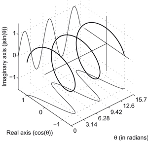
Figure 1.14

Here one can see that the combination of the sine and cosine in a two-dimensional complex space forms a spiral which is called a complex exponential |a + jb| e^arg(a+jb) re^θ = r cos(θ) + jr sin(θ) where r is the radius, or modulus of the spiral and θ is the phase or rotation of the spiral. Thus a = r cos(θ) and b = r sin(θ). The modulus of and the argument of

Using these simple relationships it is possible to have the following arithmetic rules:

Addition /subtraction (a + jb) ± (c + jd) = (a ± c) + j(b ± d), with the ± applied respectively.

Multiplication (a + jb) (c + jd) = (ac − bd) + j(ad + bc). Note: j x j = −1

Division

Note: inverting the sign of the imaginary part makes the complex conjugate of the complex number.

Adding and subtracting the complex representation of acoustic sources, of the same frequency, naturally handles their phase differences. Multiplying the complex representation of an acoustic source by a complex number can determine the effect of a filter or propagation delay. For more details see most engineering mathematics textbooks.

Example 1.9

The sound at a particular point consists of a main loudspeaker signal and a reflection at the same amplitude that has been delayed by 1 millisecond. What is the pressure amplitude at this point at 250 Hz, 500 Hz and 1 kHz?

The equation for pressure at a point due to a single frequency is given by the equation:

Pat a point =	P_{sound amplitude} sin(2πft) or P_{sound amplitude} (360°ft)
Where f =	the frequency (in HZ)
and t =	the time (in s)

Note the multiplier of 2π, or 360°, within the sine function is required to express accurately the position of the wave within the cycle. Because a complete rotation occurs every cycle, one cycle corresponds to a rotation of 360 degrees, or, more usually, 2π radians. This representation of frequency is called angular frequency (1 Hz [cycle per second] = 2π radians per second).

The effect of the delay on the difference in path lengths alters the time of arrival of one of the waves, and so the pressure at a point due to a single frequency delayed by some time, т, is given by the equation:

Add the delayed and undelayed sine waves together to give:

Assuming that the delayed and undelayed signals are of the same amplitude this can be reexpressed as:

The cosine term in this equation is determined by the delay and frequency, and the sine term represents the original wave slightly delayed. Thus we can express the combined pressure amplitude of the two waves as:

Using the above equation we can calculate the effect of the delay on the pressure amplitude at the three different frequencies as:

These calculations show that the summation of correlated sources can be strongly frequency dependent and can vary between zero and twice the wave pressure amplitude.

However, the addition of uncorrelated components always results in an increase in level without any of the cancellation effects that correlated sources suffer. Because of the lack of cancellation effects, the spatial variation in the sum of uncorrelated sources is usually much less than that of correlated ones, as the result only depends on the amplitude of the sources. As an example let us consider the effect of adding together several uncorrelated sources of the same amplitude.

How does the addition of sources affect the sound pressure level (SPL), the sound power level (SWL), and the sound intensity level (SIL)? For the SWL and SIL, because we are adding powers, the results will be the same whether the sources are correlated or not. However, for SPL, there will be a difference between the correlated and uncorrelated results. The main difficulty that arises when these measures are used to calculate the effect of combining sound sources is confusion over the correct use of decibels during the calculation.

Example 1.10

Calculate the increase in signal level when two vocalists sing together at the same level and when a choir of N vocalists sing together, also at the same level.

The total level from combining several uncorrelated sources together is given by Equation 1.28 as:

For N sources of the same amplitude this can be simplified to:

Thus the increase in level, for uncorrelated sources of equal amplitude, is proportional to the square root of the number of sources. In the case of just two sources this gives:

1.3.3 Adding Decibels Together

Decibels are power ratios expressed on a logarithmic scale and this means that adding decibels together is not the same as adding the sources’ amplitudes together. This is because adding logarithms together is equivalent to the logarithm of the product of the quantities. Clearly this is not the same as a simple summation!

When decibel values are to be added together, it is important to convert them back to their original ratios before carrying out the addition. If a decibel result of the summation is required, then the sum must be converted back to decibels after the summation has taken place. To make this clearer let us look at Example 1.11.

There are some areas of sound level calculation where the fact that the addition of decibels represents multiplication is an advantage. In these situations the result can be expressed as a multiplication, and so can be expressed as a summation of decibel values. In other words, decibels can be added when the underlying sound level calculation is a multiplication. In this context the decibel representation of sound level is very useful, as there are many acoustic situations in which the effect on the sound wave is multiplicative, for example the attenuation of sound through walls or their absorption by a surface. To make use of decibels in this context let us consider Example 1.12.

Example 1.11

Calculate the increase in signal level when two vocalists sing together, one at 69 dB and the other at 71 dB SPL.

From Equation 1.20 the SPL of a single source is:

For multiple, uncorrelated, sources this will become:

We must substitute the pressure squared values that the singers’ SPLs represent. These can be obtained with the following equation:

where p_ref² = 4 × 10⁻¹⁰ N² m⁻⁴

Substituting in our two SPL values gives:

and

Substituting these two values into Equation 1.29 gives the result as:

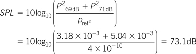
Note that the combined sound level is only about 2 dB more than the louder of the two sounds and not 69 dB greater, which is the result that would be obtained if the SPLs were added directly in decibels.

Example 1.12

Calculate the increase in the sound pressure level (SPL) when two vocalists sing together at the same level and when a choir of N vocalists sing together, also at the same level.

The total level from combining several uncorrelated single sources is given by:

This can be expressed in terms of the SPL as:

In this equation the first term simply represents the SPL of a single source, and the addition of the decibel equivalent of the square root of the number of sources represents the increase in level due to the multiple sources. So this equation can be also expressed as:

SPL_{N uncorrelated} = SPL_{single source} +10log₁₀(N)

This equation will give the total SPL for N uncorrelated sources of equal level. For example, 10 sources will raise the SPL by 10 dB, since 10log(10) = 10.

In the case of two singers the above equation becomes:

SPL_{N uncorrelated} =SPL_{single source} =10log₁₀(2) = SPL_{single source} +3 dB

So the summation of two uncorrelated sources increases the sound pressure level by 3 dB.

1.4 The Inverse Square Law

So far we have only considered sound as a disturbance that propagates in one direction. However, in reality sound propagates in three dimensions. This means that the sound from a source does not travel on a constant beam; instead it spreads out as it travels away from the radiating source, as shown in Figure 1.10.

As the sound spreads out from a source it gets weaker. This is not due to it being absorbed but due to its energy being spread more thinly. Figure 1.15 gives a picture of what happens. Consider a half blown-up spherical balloon which is coated with honey to a certain thickness. If the balloon is blown up to double its radius, the surface area of the balloon would have increased fourfold.

Figure 1.15 The honey and balloon model of the inverse square law for sound.

As the amount of honey has not changed it must therefore have a quarter of the thickness that it had before. The sound intensity from a source behaves in an analogous fashion in that every time the distance from a sound source is doubled the intensity reduces by a factor of four, that is, there is an inverse square relationship between sound intensity and the distance from the sound source. The area of a sphere is given by the equation

A_sphere = 4πr²

The sound intensity is defined as the power per unit area. Therefore the sound intensity as a function of distance from a sound source is given by:

where I =	the sound intensity (in W m^–2)
W_source =	the power of the source (in W)
and r =	the distance from the source (in m)

Equation 1.30 shows that the sound intensity for a sound wave that spreads out in all directions from a source reduces as the square of the distance. Furthermore this reduction in intensity is purely a function of geometry and is not due to any physical absorption process. In practice, there are sources of absorption in air, for example impurities and water molecules, or smog and humidity. These sources of absorption have greater effect at high frequencies and, as a result, sound not only gets quieter but also gets duller as one moves away from a source. The amount of excess attenuation is dependent on the level of impurities and humidity, and is therefore variable.

From these results we can see that the sound at 1 m from a source is 11 dB less than the sound power level at the source. Note that the sound intensity level at the source is, in theory, infinite because the area for a point source is zero. In practice, all real sources have a finite area so the intensity at the source is always finite. We can also see that the sound intensity level reduces by 6 dB every time we double the distance; this is a direct consequence of the inverse square law and is a convenient rule of thumb. The reduction in intensity of a source with respect to the logarithm of distance is plotted in Figure 1.16 and shows the 6 dB per doubling of distance relationship as a straight line except when one is very close to the source. In this situation the fact that the source is finite in extent renders Equation 1.30 invalid. As an approximate rule the nearfield region occurs within the radius described by the physical size of the source. In this region the sound field can vary wildly depending on the local variation of the vibration amplitudes of the source.

Figure 1.16 Sound intensity as a function of distance from the source.

Example 1.13

A loudspeaker radiates one hundred milliwatts (100 mW). What is the sound intensity level (SIL) at a distance of 1 m, 2 m and 4 m from the loudspeaker? How does this compare with the sound power level (SWL) at the loudspeaker?

The sound power level can be calculated from Equation 1.19 and is given by:

The sound intensity at a given distance can be calculated using Equations 1.18 and 1.30 as:

This can be simplified to give:

which can be simplified further to:

This equation can then be used to calculate the intensity level at the three distances as:

A milliwatt is one thousandth of a watt (10⁻³ watts).

Equation 1.30 describes the reduction in sound intensity for a source which radiates in all directions. However, this is only possible when the sound source is well away from any surfaces that might reflect the propagating wave. Sound radiation in this type of propagating environment is often called the free field radiation, because there are no boundaries to restrict wave propagation.

1.4.1 The Effect of Boundaries

But how does a boundary affect Equation 1.30? Clearly many acoustic contexts involve the presence of boundaries near acoustic sources, or even all the way round them in the case of rooms, and some of these effects will be considered in Chapter 6. However, in many cases a sound source is placed on a boundary, such as a floor. In these situations the sound is radiating into a restricted space, as shown in Figure 1.17. However, despite the restriction of the radiating space, the surface area of the sound wave still increases in proportion to the square of the distance, as shown in Figure 1.17. The effect of the boundaries is merely to concentrate the sound power of the source into a smaller range of angles. This concentration can be expressed as an extra multiplication factor in Equation 1.30. Therefore the equation can be rewritten as:

Figure 1.17 The inverse square law for sound at boundaries.

where I_{directive source} =	the sound intensity (in W m^–2)
Q =	the directivity of the source (compared to a sphere)
W_source =	the power of the source (in W)
and r =	the distance from the source (in m)

Equation 1.32 can be applied to any source of sound which directs its sound energy into a restricted solid angle which is less than a sphere. Obviously the presence of boundaries is one means of restriction, but other techniques can also achieve the same effect. For example, the horn structure of brass instruments results in the same effect. However, it is important to remember that the sound intensity of a source reduces in proportion to the square of the distance, irrespective of the directivity.

The effect of having the source on a boundary can also be calculated; as an example let us examine the effect of boundaries on the sound intensity from a loudspeaker.

From these calculations we can see that each boundary increases the sound intensity at a point by 3 dB, due to the increased directivity. Note that one cannot use the above equations on more than three boundaries because then the sound can no longer expand without bumping into something. We shall examine this subject in more detail in Chapter 6. However, it is possible to have directivities of greater than 8 using other techniques. For example, horn loudspeakers with a directivity of 50 are readily available as a standard product from public address loudspeaker manufacturers.

1.5 Sound Interactions

So far we have only considered sound in isolation and we have seen that sound has velocity, frequency, and wavelength, and reduces in intensity in proportion to the square of the distance from the source. However, sound also interacts with physical objects and other sound waves, and is affected by changes in the propagating medium. The purpose of this section is to examine some of these interactions as an understanding of them is necessary in order to understand both how musical instruments work and how sound propagates in buildings.

Example 1.14

A loudspeaker radiates 100 mW. Calculate the sound intensity level (SIL) at a distance of 2 m from the loudspeaker when it is mounted on 1, 2 and 3 mutually orthogonal boundaries.

The sound intensity at a given distance can be calculated using Equations 1.18 and 1.32 as:

which can be simplified to give:

This is similar to Equation 1.32 except for the addition of the term for the directivity, Q. The presence of 1, 2 and 3 mutually orthogonal boundaries converts the sphere to a hemisphere, half hemisphere and quarter hemisphere, which corresponds to a Q of 2, 4 and 8, respectively. As the only difference between the results with the boundaries is the term in Q, the sound intensity level at 2 m can be calculated as:

1.5.1 Superposition

When sounds destructively interfere with each other they do not disappear. Instead they travel through each other. Similarly, when they constructively interfere they do not grow but simply pass through each other. This is because although the total pressure, or velocity component, may lie anywhere between zero and the sum of the individual pressures or velocities, the energy flow of the sound waves is still preserved and so the waves continue to propagate. Thus the pressure or velocity at a given point in space is simply the sum, or superposition, of the individual waves that are propagating through that point, as shown in Figure 1.18. This characteristic of sound waves is called linear superposition and is very useful as it allows us to describe, and therefore analyze, the sound wave at a given point in space as the linear sum of individual components.

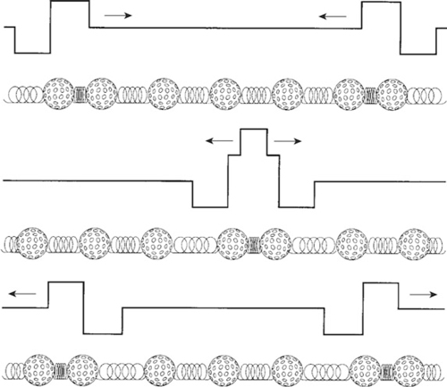
Figure 1.18 Superposition of a sound wave in the golf ball and spring model.

1.5.2 Sound Refraction

This is analogous to the refraction of light at the boundary of different materials. In the optical case refraction arises because the speed of light is different in different materials; for example it is slower in water than it is in air. In the acoustic case refraction arises for the same reasons, because the velocity of sound in air is dependent on the temperature, as shown in Equation 1.5.

Consider the situation shown in Figure 1.19 where there is a boundary between air at two different temperatures. When a sound wave approaches this boundary at an angle, then the direction of propagation will alter according to Snell’s law, that is, using Equation 1.5:

Figure 1.19 Refraction of a sound wave (absolute temperature in medium₁ is T₁ and in medium₂ is T₂; velocity in medium₁ is y_T1 and in medium₂ is y_T2).

where θ₁, θ₂ =	the propagation angles in the media
C_T1, C_T2 =	the velocities of the sound waves in the two media
and T₁, T₂ =	the absolute temperatures of the two media

Thus the change in direction is a function of the square root of the ratio of the absolute temperatures of the air on either side of the boundary. As the speed of sound increases with temperature one would expect to observe that when sound moves from colder to hotter air it would be refracted away from the normal direction, and that it would refract toward the normal when moving from hotter to colder air. This effect has some interesting consequences for outdoor sound propagation.

Normally the temperature of air reduces as a function of height and this results in the sound wave being bent upward as it moves away from a sound source, as shown in Figure 1.20. This means that listeners on the ground will experience a reduction in sound level as they move away from the sound, which reduces more quickly than the inverse square law would predict. This is a helpful effect for reducing the effect of environmental noise nuisance. However, if the temperature gradient increases with height then instead of being bent up the sound waves are bent down, as shown in Figure 1.21. This effect can often happen on summer evenings and results in a greater sound level at a given distance than predicted by the inverse square law. This behavior is often responsible for the pop concert effect where people living some distance away from the concert experience noise disturbance whereas people living nearer the concert do not experience the same level of noise.

Figure 1.20 Refraction of a sound wave due to a normal temperature gradient.

Figure 1.21 Refraction of a sound wave due to an inverted temperature gradient.

Refraction can also occur at the boundaries between liquids at different temperatures, such as water, and in some cases the level of refraction can result in total internal reflection. This effect is sometimes used by submarines to hide from the sonar of other ships; it can also cause the sound to be ducted between two boundaries and in these cases sound can cover large distances. It is thought that these mechanisms allow whales and dolphins to communicate over long distances in the ocean.

Wind can also cause refraction effects because the velocity of sound within the medium is unaffected by the velocity of the medium. The velocity of a sound wave in a moving medium, when viewed from a fixed point, is the sum of the two velocities, so that it is increased when the sound is moving with the wind and is reduced when it is moving against the wind. As the velocity of air is generally less at ground level compared with the velocity higher up (due to the effect of the friction of the ground), sound waves are bent upward or downward depending on their direction relative to the wind. The degree of direction change depends on the rate of change in wind velocity as a function of height; a faster rate of change results in a greater direction change. Figure 1.22 shows the effect of wind on sound propagation.

Figure 1.22 Refraction of a sound wave due to a wind velocity gradient.

1.5.3 Sound Absorption

Sound is absorbed when it interacts with any physical object. One reason is the fact that when a sound wave hits an object then that object will vibrate, unless it is infinitely rigid. This means that vibrational energy is transferred from the sound wave to the object that has been hit. Some of this energy will be absorbed because of the internal frictional losses in the material that the object is made of. Another form of energy loss occurs when the sound wave hits, or travels through, some porous material. In this case there is a very large surface area of interaction in the material, due to all the fibers and holes. There are frictional losses at the surface of any material due to the interaction of the velocity component of the sound wave with the surface. A larger surface area will have a higher loss, which is why porous materials such as cloth or rock-wool absorb sound waves strongly.

1.5.4 Sound Reflection from Hard Boundaries

Sound is also reflected when it strikes objects and we have all experienced the effect as an echo when we are near a large hard object such as a cliff or large building. There are two main situations in which reflection can occur.

In the first case the sound wave strikes an immovable object, or hard boundary, as shown in Figure 1.23. At the boundary between the object and the air the sound wave must have zero velocity, because it can’t move the wall. This means that at that point all the energy in the sound is in the compression of the air, or pressure. As the energy stored in the pressure cannot transfer in the direction of the propagating wave, it bounces back in the reverse direction, which results in a change of phase in the velocity component of the wave.

Figure 1.23 Reflection of a sound wave due to a rigid barrier.

Figure 1.23 shows this effect using our golf ball and spring model. One interesting effect occurs due to the fact that the wave has to change direction and to the fact that the spring connected to the immovable boundary is compressed twice as much compared with a spring well away from the boundary. This occurs because the velocity components associated with the reflected (bounced back) wave are moving in contrary motion to the velocity components of the incoming wave, due to the change of phase in the reflected velocity components. In acoustic terms this means that while the velocity component at the reflecting boundary is zero, the pressure component is twice as large.

1.5.5 Sound Reflection from Bounded to Unbounded Boundaries

In the second case the wave moves from a bounded region, for example a tube, into an unbounded region, for example free space, as shown in Figure 1.24. At the boundary between the bounded and unbounded regions the molecules in the unbounded region find it a lot easier to move than in the bounded region. The result is that, at the boundary, the sound wave has a pressure component which is close to zero and a large velocity component. Therefore at this point all the energy in the sound is in the kinetic energy of the moving air molecules—in other words, the velocity component. Because there is less resistance to movement in the unbounded region, the energy stored in the velocity component cannot transfer in the direction of the propagating wave due to there being less “springiness” to act on. Therefore the momentum of the molecules is transferred back to the “springs” in the bounded region which pushed them in the first place, by stretching them still further.

Figure 1.24 Refection of a sound wave due to bounded–unbounded transition.

This is equivalent to the reflection of a wave in the reverse direction in which the phase of the wave is reversed, because it has started as a stretching of the “springs,” or rarefaction, as opposed to a compression. Figure 1.24 shows this effect using the golf ball and spring model in which the unbounded region is modeled as having no springs at all. An interesting effect also occurs in this case, due to the fact that the wave has to change direction. That is, the mass that is connected to the unbounded region is moving with twice the velocity compared to masses well away from the boundary. This occurs because the pressure components associated with the reflected (bounced back) wave are moving in contrary motion to the pressure components of the incoming wave, due to the change of phase in the reflected pressure components. In acoustic terms this means that while the pressure component at the reflecting boundary is zero, the velocity component is twice as large.

To summarize, reflection from a solid boundary results in a reflected pressure component that is in phase with the incoming wave, whereas reflection from a bounded to unbounded region results in a reflected pressure component which is in antiphase with the incoming wave. This arises due to the difference in acoustic impedance at the boundary. In the first case the impedance of the boundary is greater than the propagating medium and in the second case it is smaller. For angles of incidence on the boundary, away from the normal, the usual laws of reflection apply.

1.5.6 Sound Interference

We saw earlier that when sound waves come from correlated sources then their pressure and associated velocity components simply add. This means that the pressure amplitude could vary between zero and the sum of the pressure amplitudes of the waves being added together, as shown in Example 1.9. Whether the waves add together constructively or destructively depends on their relative phases and this will depend on the distance each one has had to travel. Because waves vary in space over their wavelength then the phase will also spatially vary. This means that the constructive or destructive addition will also vary in space.

Free space is a region in which the sound wave is free to travel in any direction. That is, there are no obstructions or changes in the propagation medium to affect its travel. Therefore, free space is a form of unbounded region. However, not all bounded regions are free space. For example, the wave may be coming out of a tube in a very large wall. In this case there is a transition between a bounded and an unbounded region but it is not free space, because the wave cannot propagate in all directions.

Consider the situation shown in Figure 1.25, which shows two correlated sources feeding sound into a room. When the listening point is equidistant from the two sources (P1), the two sources add constructively because they are in phase. If one moves to another point (P2), which is not equidistant, the waves no longer necessarily add constructively. In fact, if the path difference is equal to half a wavelength then the two waves will add destructively and there will be no net pressure amplitude at that point. This effect is called interference, because correlated waves interfere with each other; note that this effect does not occur for uncorrelated sources.

Figure 1.25 Interference from correlated sources.

The relative phases of the waves depend on their path difference or relative delays. Because of this the pattern of constructive and destructive interferences depends strongly on position, as shown in Figure 1.26. Less obviously the interference is also strongly dependent on frequency. This is because the factor that determines whether or not the waves add constructively or destructively is the relative distance from the listening point to the sources measured in wavelengths (λ). Because the shape of the amplitude response looks a bit like the teeth of a comb, the frequency domain effect of interference is often referred to as “comb filtering.” As the wavelength is inversely proportional to frequency one would expect to see the pattern of interference vary directly with frequency, and this is indeed the case.

Figure 1.26 Effect of position on interference at a given frequency.

Figure 1.27 shows the amplitude that results when two sources of equal amplitude but different relative distances are combined. The amplitude is plotted as a function of the relative distance measured in wavelengths (λ). Figure 1.27 shows that the waves constructively interfere when the relative delay is equal to a multiple of a wavelength, and that they interfere destructively at multiples of an odd number of half wavelengths. As the number of wavelengths for a fixed distance increases with frequency, this figure shows that the interference at a particular point varies with frequency. If the two waves are not of equal amplitude then the interference effect is reduced, also as shown in Figure 1.27. In fact once the interfering wave is less than one eighth of the other wave then the peak variation in sound pressure level is less than 1 dB.

Figure 1.27 Effect of frequency, or wavelength, on interference at a given position. The ratios refer to the relative amplitudes of the two waves.

There are several acoustical situations which can cause interference effects. The obvious ones are when two loudspeakers radiate the same sound into a room, or when the same sound is coupled into a room via two openings which are separated. A less obvious situation is when there is a single sound source spaced away from a reflecting boundary, either bounded or unbounded. In this situation an image source is formed by the reflection and thus there are effectively two sources available to cause interference, as shown in Figure 1.28. This latter situation can often cause problems for recording or sound reinforcement due to a microphone picking up a direct and reflected sound component and so suffering interference.

Figure 1.28 Interference arising from reflections from a boundary.

1.5.7 Standing Waves at Hard Boundaries (Modes)

The linear superposition of sound can also be used to explain a wave phenomenon known as “standing waves,” which is applicable to any form of sound wave. Standing waves occur when sound waves bounce between reflecting surfaces. The simplest system in which this can occur consists of two reflecting boundaries as shown in Figure 1.30. In this system the sound wave shuttles backward and forward between the two reflecting surfaces.

Figure 1.30 Reflection of a sound wave between two parallel surfaces.

Example 1.15

Two loudspeakers are one meter apart and radiate the same sound pressure level. A listener is two meters directly in front of one speaker on a line which is perpendicular to the line joining the two loudspeakers; see Figure 1.29. What are the first two frequencies at which destructive interference occurs? When does the listener first experience constructive interference, other than at very low frequencies?

Figure 1.29 Interference at a point due to two loudspeakers.

First work out the path length difference using Pythagoras’ theorem:

The frequencies at which destructive interference will occur will be λ/2 and 3λ/2. The frequencies at which this will happen will be when these wavelengths equal the path length difference. Thus the first frequency can be calculated using:

The second frequency will occur at 3 times the first and so can be given by:

The frequency at which the first constructive interference happens will occur at twice the frequency of the first destructive interference which will be:

If the listener were to move closer to the center line of the speakers then the relative delays would reduce and the frequencies at which destructive interference occurs would get higher. In the limit when the listener was equidistant the interference frequencies would be infinite, that is, there would be no destructive interference.

If we used complex numbers to represent the speaker outputs, say Ls₁ and Ls₂, then we could account for the phase shift due to the propagation delay by multiplying the speaker outputs by:

θ_delay (k) = e^{−jkdistance}

multiplying distance by k, the wavenumber, defines the number of cycles the wave is delayed by. So if the two distances were d₁ and d₂ respectively, the result at the listener position would be:

and one could find the magnitude and phase of the composite result by taking the argument and magnitude of the result. Note that because the phase depends on k, the result is frequency dependent.

At most frequencies the distance between the two boundaries will not be related to the wavelength and so the compression and rarefaction peaks and troughs will occupy all positions between the two boundaries, with equal probability, as shown in Figure 1.31. However, when the wavelength is related to the distance between the two boundaries the wave keeps tracing the same path as it travels between the two boundaries. This means that the compressions and rarefactions always end up in the same position between the boundaries.

Figure 1.31 A non-stationary sound wave between two parallel surfaces.

Thus the sound wave will appear to be stationary between the reflecting boundaries, and so is called a standing wave, or, more precisely, a resonant mode. It is important to realize that the wave is still moving at its normal speed—it is merely that, like a toy train, the wave endlessly retraces the same positions between the boundaries with respect to the wavelength, as shown in Figure 1.32.

Figure 1.32 The pressure components of a standing wave between two hard boundaries; this is known as a “resonant mode.”

Figures 1.32 and 1.33 show the pressure and velocity components respectively of a standing wave between two hard reflecting boundaries. In this situation the pressure component is a maximum and the velocity component is a minimum at the two boundaries. The largest wave that can fit these constraints is a half wavelength and this sets the lowest frequency at which a standing wave can exist for a given distance between reflectors, which can be calculated using the following equation:

Figure 1.33 The velocity components of a standing wave between two hard boundaries.

where f_lowest =	the standing wave frequency (in Hz)
L =	the distance between the boundaries (in m)
λ =	the wavelength (in m)
and c =	the velocity of sound (in ms^–1)

Strictly speaking the standing waves we are discussing here should be called resonant modes. This is because it is possible to set up a standing wave without the use of two boundaries. For example, one could use two loudspeakers spaced apart and no boundaries to get a standing wave at discrete frequencies. One can do the same with one loudspeaker, or sound source, and one boundary.

Any multiple of half wavelengths will also fit between the two reflectors, and so there is in theory an infinite number of frequencies at which standing waves occur which are all multiples of f_lowest. These can be calculated directly using:

where f_n =	the nth standing wave frequency (in Hz)
and n =	1, 2, …, ∞

An examination of Figures 1.32 and 1.33 shows that there are points of maximum and minimum amplitude of the pressure and velocity components. For example, in Figure 1.31 the pressure component’s amplitude is a maximum at the two boundaries and at the midpoint, while in Figure 1.33 the velocity component is zero at the two boundaries and the midpoint. The point at which the pressure amplitude is zero is called a pressure node and the maximum points are called pressure antinodes. Note that as the number of half wavelengths in the standing waves increases then the number of nodes and antinodes increases, and for hard reflecting boundaries the number of pressure nodes is equal to, and the number of pressure antinodes is one more than, the number of half wavelengths. Velocity nodes and antinodes also exist, and they are always complementary to the pressure nodes, that is, a velocity antinode occurs at a pressure node and vice versa, as shown in Figure 1.34. This happens because the energy in the traveling wave must always exist at a pressure node carried in the velocity component, and at a velocity node the energy is carried in the pressure component.

Figure 1.34 The pressure and velocity components of a standing wave between two hard boundaries.

1.5.8 Standing Waves at other Boundaries

There are two other pairs of boundary arrangements which can support standing waves. The first, shown in Figure 1.35 and 1.36, is the case of a bounded-to-unbounded propagation boundary at both ends. An example would be a tube or pipe which is open at both ends. In this situation the pressure component is zero at the boundaries whereas the velocity component is at a maximum, as shown in Figures 1.35 and 1.36. Like the hard reflecting boundaries the minimum frequency for a standing wave occurs when there is precisely half a wavelength between the two boundaries, and at all subsequent multiples of this frequency. This means that Equation 1.35 can also be used to calculate the standing wave frequencies for this boundary arrangement.

Figure 1.35 The pressure components of a standing wave between two bound–unbound boundaries.

Figure 1.36 The velocity components of a standing wave between two bound–unbound boundaries.

Example 1.16

Calculate the first two modal (standing wave) frequencies for a pipe 98.5 cm long, and open at both ends.

As this is a system with identical boundaries we can use Equation 1.35 to calculate the two frequencies as:

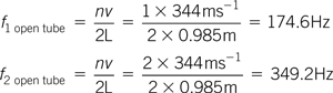
These two frequencies correspond to the notes F3 and F4, which differ by an octave.

The second is more interesting and consists of one hard boundary and one bound–unbound boundary, and is shown in Figures 1.37 and 1.38. In this situation there is a pressure node at the bound–unbound boundary and a pressure antinode at the hard boundary. The effect of this is to allow a standing wave to exist when there is only an odd number of quarter wavelengths between the two boundaries.

Figure 1.37 The pressure components of a standing wave between mixed boundaries.

Figure 1.38 The velocity components of a standing wave between two mixed boundaries.

A standing wave cannot exist with even numbers of quarter wavelengths as this would require a pressure node or antinode at both ends as shown in Figures 1.32 and 1.35. The frequencies which can support standing waves exist at odd multiples of the lowest standing wave frequency. This can be expressed algebraically as:

where f_n =	the nth standing wave frequency (in Hz)
and n =	0, 1, 2, …, ∞

Figures 1.37 and 1.38 demonstrate the standing wave for n = 2 which is five times the lowest supported standing wave frequency. Standing waves can also occur for any type of wave propagation. A transverse wave on a string which is clamped at the ends has standing waves which can be predicted using Equation 1.36, provided one uses the propagation velocity of the transverse wave for v.

Standing waves in an acoustic context are often called the modes of a given system; the lowest frequency standing wave is known as the “first order mode,” and the multiples of this are higher order modes. So the third order mode of a system is the third lowest frequency standing wave pattern which can occur in it. Standing waves are also not just restricted to situations with two parallel reflecting boundaries. In fact any sequence of reflections or refractions which returns the wave back to the beginning of its phase will support a standing wave or mode. This can happen in one, two and three dimensions and with any form of wave propagation. The essential requirement is a cyclic path in which the time of propagation results in the wave traveling around this path in phase with the previous time round. Figure 1.39 shows an example of a two-dimensional standing wave.

Figure 1.39 A two-dimensional standing wave.

Example 1.17

Calculate the first two modal (standing wave) frequencies for the same pipe as in Example 1.16 with one end closed.

As this is a system with non-identical boundaries we must use Equation 1.36 to calculate the two frequencies as:

In this case the first mode is at half the frequency of the pipe, that is open at both ends, and an octave below on the musical scale, which is F2. The second mode is now at three times the lowest mode, which is approximately equal to C4 on the musical scale.

1.5.9 Sound Diffraction

We have all experienced the ability of sound to travel around the corners of a building or other objects. This is due to a process, known as “diffraction,” in which the sound bends around objects, as shown in Figure 1.40. Diffraction occurs because the variations in air pressure, due to the compressions and rarefactions in the sound wave, cannot go abruptly to zero after passing the edge of an object. This is because there is interaction between the adjacent molecules that are propagating the wave. In order to allow the compressions and rarefactions to die out gracefully in the boundary between the wave and the shadow, there must be a region in which part of the propagating wave changes direction, and it is this bent part of the wave that forms the diffracted component.

Figure 1.40 Diffraction around an object.

The degree of diffraction depends on wavelength because it effectively takes a certain number of wavelengths for the edge of the wave to make the transition to shadow. Thus the amount of diffraction around an edge, such as a building or wall, will be greater at low and less at high frequencies. This effect is shown in Figures 1.41 and 1.42. Similar effects occur when sound has to pass through an opening, as shown in Figures 1.43 and 1.44. Here the sound wave is diffracted away from the edges of the opening. The amount of diffraction depends on the size of the opening relative to the wavelength. When the size of the wavelength is large relative to the opening the wave is diffracted strongly, and when the wavelength is small relative to the opening then the diffraction is low. The transition between the wavelength being small and large with respect to the opening occurs when the opening size is about two thirds of the wavelength ( λ).

Figure 1.41 Diffraction around an edge at low frequencies.

Figure 1.42 Diffraction around an edge at high frequencies.

Figure 1.43 Diffraction through an opening at low frequencies.

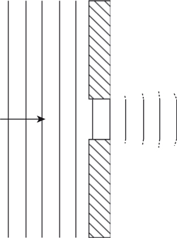
Figure 1.44 Diffraction through an opening at high frequencies.

As well as occurring through openings, diffraction also happens around solid objects; one could consider them to be anti-openings, as shown in Figures 1.45 and 1.46. Here the wave diffracts around the object and meets behind it. The effect is also a function of the size of the object with respect to the wavelength. When the size of the wavelength is large relative to the object then the wave is diffracted strongly around it and the object has little influence on the wave propagation. On the other hand, when the wavelength is small relative to the object then the diffraction is less, and the object has a significant shadow behind it; these effects are shown in Figure 1.46. The size at which an object becomes significant with respect to a wavelength is when its size is again about two thirds of a wavelength ( λ).

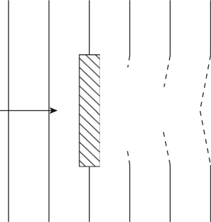
Figure 1.45 Diffraction around an object at low frequencies.

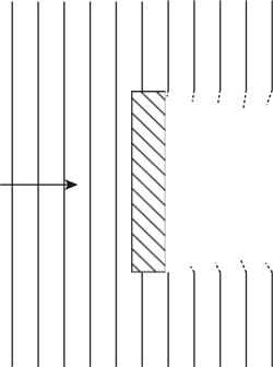
Figure 1.46 Diffraction around an object at high frequencies.

1.5.10 Sound Scattering

Sound which is incident on an object is not just diffracted around it—some of the incident energy will be reflected, or scattered, from the side facing the incident wave, as shown in Figure 1.47. As in the case of diffraction, it is the size of the object with respect to the wavelength that determines how much, and in what way, the energy is scattered. When the object is large with respect to the wavelength then most of the sound incident on the object is scattered according to the laws of reflection and there is very little spreading or diffraction of the reflected wave, as shown in Figure 1.48.

Figure 1.47 Scattering from an object at low frequencies.

Figure 1.48 Scattering from an object at high frequencies.

However, when the object is small with respect to the wavelength only a small proportion of the incident energy is scattered and there is a large amount of spreading or diffraction of the reflected wave, as shown in Figure 1.47. As in the case of diffraction, the size at which the object becomes significant is when it is about two thirds of a wavelength ( λ). Thus objects smaller than this will tend to scatter the energy in all directions whereas objects bigger than this will be more directional.

In addition to the scattering effects, interference effects happen when the scattering object is about two thirds of a wavelength ( λ) in size. This is because at this frequency both reflection from, and diffraction around, the object is occurring. In this situation the waves on the two sides of the object can influence or interact with each other. This results in enhanced reflection from, or diffraction around, the object at particular wavelengths. The precise nature of these effects depends on the interaction between the front and back of the scattering object and so will be significantly affected by its shape. Thus the variation in scattering will be different for a sphere compared with rectangular plate. As the sum of energy diffracted around the object and the scattered energy must be constant, the reflection and diffraction responses will be complementary.

1.6 Time and Frequency Domains

So far we have mainly considered a sound wave to be a sinusoidal wave at a particular frequency. This is useful as it allows us to consider aspects of sound propagation in terms of the wavelength. However, most musical sounds have a waveform that is more complex than a simple sine wave; a variety of waveforms are shown in Figure 1.49. So how can we analyze real sound waveforms, and make sense of them in acoustical terms? The answer is based on the concept of superposition and a technique called Fourier analysis.

Figure 1.49 Waveforms from musical instruments.

1.6.1 What is Fourier Theory?

Fourier analysis is a way of building up a waveform from much simpler bits. There are many ways of building up complex waveforms from simple basic shapes, like rectangles, but Fourier analysis was developed (by a French mathematician called Jean Baptiste Joseph Fourier in 1807) to solve the problem of heat diffusion in a metal bar! His idea was very simple. He built up the more complicated shapes of the functions, or waveforms, that he was studying by using the humble sine wave. He found that by adding together sine waves with different frequencies, phases and amplitudes he could, very accurately, approximate the functions he was interested in. He found that using sine waves as a basis for approximation was a very useful thing to do. For a start different sine wave frequencies were independent, from, or; more strictly, orthogonal to, each other and so could be manipulated, or used in equations, independently of each other. That is, if you solved the equations for each sine wave independently, then you had the solution for the whole waveform. As finding the solution for each sine wave was much easier, this was a great advantage. This principle—that the sum of the solutions is the same as the solution of the sum of the sine waves—is called superposition and is a powerful aspect of the Fourier approach.

Fourier further theorized that if he combined enough sine waves together he could exactly model any waveform in existence. This allowed him to develop the Fourier transform pair—two equations that provide a means of transforming the time domain into the frequency domain and back.

These techniques are useful because sometimes it’s easier to think about some processes in one domain rather than the other. For example, it’s much easier to think about filtering, resonance, and modes of vibration in the frequency domain rather than the time domain. Furthermore, the fact that the basis functions are sine waves, which have a direct physical analog, is useful when dealing with the real world. The next section gives a simple, non-mathematical introduction to Fourier analysis. More details may be found in Appendix 1 and Bracewell (1999).

1.6.2 The Spectrum of Periodic Sound Waves

Fourier theory states that any waveform can be built up by using an appropriate set of sine waves of different frequencies, amplitudes and phases. To see how this might work consider the situation shown in Figure 1.50. This shows four sine waves whose frequencies are 1F Hz, 3F Hz, 5F Hz, and 7F Hz, whose phase is zero (that is, they all start from the same value, as shown by the dotted line in Figure 1.50) and whose amplitude is inversely proportional to the frequency. This means that the 3F Hz component is 1/3 the amplitude of the component at 1F Hz, and so on. When these sine waves are added together, as shown in Figure 1.50, the result approximates a square wave, and, if more high-frequency components were added, it would become progressively closer to an ideal square wave. The higher frequency components are needed in order to provide the fast rise, and sharp corners, of the square wave.

Figure 1.50 The effect of adding several harmonically related sine waves together.

In general, as the rise time gets faster, and/or the corners get sharper, then more high-frequency sine waves are required to represent the waveform accurately. In other words we can look at a square wave as a waveform that is formed by summing together sine waves which are odd multiples of its fundamental frequency and whose amplitudes are inversely proportional to frequency. A sine wave represents a single frequency and therefore a sine wave of a given amplitude can be plotted as a single line on a graph of amplitude versus frequency. The components of a square wave plotted in this form are shown in Figure 1.51, which clearly shows that the square wave consists of a set of progressively reducing discrete sine wave components at odd multiples of the lowest frequency. This representation is called the frequency domain representation, or spectrum, of a waveform and the waveform’s amplitude versus time plot is called its time domain representation.

Figure 1.51 The frequency domain representation, or spectrum, of a square wave.

The individual sine wave components of the waveform are often called the partials of the waveform. If they are integer related, as in the square wave, then they can be called harmonics. The lowest frequency is called the fundamental, or first harmonic, and the higher frequency harmonics are labeled according to their frequency multiple relative to the fundamental. Thus the second harmonic is twice the frequency of the fundamental and so on. Partials on the other hand need not be harmonically related to the fundamental, and are numbered in their order of appearance with frequency. However, as we shall see later, this results in a waveform that is a periodic. So for the square wave the second partial is the third harmonic and the third partial is the fifth harmonic. Other waveforms have different frequency domain representations, because they are made up of sine waves of different amplitudes and frequencies. Some examples of other waveforms in both the time and frequency domains are shown in Chapter 3.

1.6.3 The Effect of Phase

The phase, which expresses the starting value of the individual sine wave components, also affects the waveshape. Figure 1.52 shows what happens to a square wave if alternate partials are subtracted rather than added, and this is equivalent to changing the phase of these components by 180°; that is, alternate frequency components start from halfway around the circle compared with the other components, as shown by the dotted line in Figure 1.52. However, although the time domain waveform is radically different the frequency domain is very similar, as the amplitudes are identical—only the phase of some of the harmonics has changed.

Figure 1.52 The effect of adding harmonically related sine waves together with different phase shifts.

Interestingly, in many cases, the resulting wave is perceived as sounding the same, even though the waveform is different. This is because the ear, as we will see later, appears to be less sensitive to the phase of the individual frequency compared with the relative amplitudes. However, if the phase changes are extreme enough we can hear a difference (see Schroeder, 1975). Because of this, often only the amplitudes of the frequency components are plotted in the spectrum and, in order to handle the range of possible amplitudes and because of the way we perceive sound, the amplitudes are usually plotted as decibels. For example, Figure 4.24 in Chapter 4 shows the waveform and spectrum plotted in this fashion for middle C played on a clarinet and tenor saxophone.

1.6.4 The Spectrum of Non-Periodic Sound Waves

So far, only the spectrum of waveforms which are periodic, that is, have pitch, has been considered. However, some instruments, especially percussion, do not have pitch and hence are non-periodic, or aperiodic. How can we analyze these instruments in terms of a basic waveform, such as a sine wave, which is inherently periodic? The answer is shown in Figure 1.53. Here the square wave example discussed earlier has had four more sine waves added to it. However, these sine waves are between the harmonics of the square wave and so are unrelated to the period, but they do start off in phase with the harmonics. The effect of these other components is to start canceling out the repeat periods of the square waves, because they are not related in frequency to them. By adding more components which sit in between the harmonics, this cancellation of the repeats becomes more effective so that when in the limit, the whole space between the harmonics is filled with sine wave components of the appropriate amplitude and phase. These extra components will add constructively only at the beginning of the waveform and will interfere with successive cycles due to their different frequencies. Therefore, in this case, only one square wave will exist.

Figure 1.53 The effect of adding several non-harmonically related sine waves together.

Thus the main difference between the spectrum of periodic and aperiodic waveforms is that periodic waveforms have discrete partials, which can be represented as lines in the spectrum with a spacing that is inversely proportional to the period of the waveform. Aperiodic waveforms by contrast will have a spectrum which is continuous and therefore does not have any discrete components. However, the envelope of the component amplitudes as a function of frequency will be the same for both periodic and aperiodic waves of the same shape, as shown in Figure 1.54. Figure 3.6 in Chapter 3 shows the aperiodic waveform and spectrum of a brushed snare.

Figure 1.54 The frequency domain representation, or spectrum, of an aperiodic square wave.

1.7 Analyzing Spectra

Because the spectrum of a sound is an important part of the way we perceive it, there is often a need to look at the spectrum of a real signal. The way this is achieved is to use a bank of filters, as shown in Figure 1.55.

Figure 1.55 A filter bank for analyzing spectra.

1.7.1 Filters and Filter Types

A filter is a device which separates out a portion of the frequency spectrum of a sound signal from the total; this is shown in Figure 1.56. There are four basic types of filter, which are classified in terms of their effect as a function of signal frequency. This is known as the filters’ “frequency response.” These basic types of filter are as follows:

Low-pass: The filter only passes frequencies below a frequency known as the filter’s “cut-off frequency.”
High-pass: The filter only passes frequencies above the cut-off frequency.
Band-pass: The filter passes a range of frequencies between two cutoff frequencies. The frequency range between the cut-off frequencies is the filter’s “bandwidth.”
Band-reject: The filter rejects a range of frequencies between two cutoff frequencies.

Figure 1.56 The effect of different filter types.

The effects of these four types of filter are shown in Figure 1.56 and one can see that a bank of band-pass filters are the most appropriate for analyzing the spectrum of a sound wave. Note that although practical filters have specified cut-off frequencies which are determined by their design, they do not cut off instantly as the frequency changes. Instead they take a finite frequency range to attenuate the signal.

The effect of a filter on a spectrum is multiplicative in that the output spectrum after filtering is the product of the filter’s frequency response with the input signal’s spectrum. Thus we can easily determine the effect of a given filter on a signal’s spectrum. This is a useful technique which can be applied to the analysis of musical instruments, as we shall see later, by treating some of their characteristics as a form of filtering. In fact, filtering can be carried out using mechanical, acoustical and electrical means, and many instruments perform some form of filtering on the sounds they generate (see Chapter 4).

1.7.2 Filter Time Responses

There is a problem, however, with filtering a signal in order to derive the spectrum and this is the effect of the filter on the time response of the signal. Most filters have a time response due to the fact that they do not allow all frequencies to pass through—if they did they wouldn’t be filters! Why do such filters have a time response? The answer can be obtained by reconsidering the Fourier analysis approach to analyzing a sound signal. For example, if a signal is low-pass filtered such that the maximum frequency is F_max, then there can be no sine waves with a frequency greater than F_max in the output. As a sine wave has a slope which is a function of its frequency, the maximum rate of change in the output will be determined by the frequency of F_max. Any faster rate of change would require higher frequency sine waves that are no longer present, as shown in Figure 1.57 which shows the effect of low-pass filtering a square wave such that only the first two partials are passed, as shown in Figure 1.58.

Figure 1.57 The effect of low-pass filtering a square wave on the waveform.

Figure 1.58 The spectral effect of low-pass filtering a square wave.

There is a special type of filter known as the “all-pass filter.” This is not a piece of wire! It is a filter that changes the phase of the signal’s frequency components without affecting their amplitude. Because the phases have been changed there is also an associated time response.

A similar argument can used for band-pass filters. In this case there is a maximum range of frequencies that can be passed around a given frequency. Although the sine waves corresponding to the band-pass frequencies will be passed, and they may be at quite a high frequency, their amplitude envelope cannot vary quickly, as shown in Figure 1.59. This is because the speed of variation of the envelope depends on the number of, and total frequency occupied by, the sine wave components in the output of the filter, as shown in Figure 1.60. As it is the amplitude variation of the output of a bandpass filter that carries the information, it too has an inherent time response which is a function of its bandwidth.

Figure 1.59 The effect of band-pass filtering on a square wave envelope.

Figure 1.60 The spectral effect of bandpass filtering a square wave envelope.

Thus all filters have a time response which is a function of the frequency range or bandwidth of the signals that they pass. Note that this is an inherent problem that cannot be solved by technology. The time response of a filter is inversely proportional to the bandwidth so a narrow-band filter has a slow rise and fall time whereas a wide-band filter has faster rise and fall times. In practice this effect means that if the frequency resolution of the spectral analysis is good, implying the use of narrow-band analysis filters, then the time response is poor and there is significant smearing of the signal. On the other hand if the time response is good then the frequency resolution will be poor, because the filter bandwidths will have to be wider.

1.7.3 Time Responses of Acoustic Systems

This argument can be reversed to show that when the output of an acoustic system, such as a musical instrument, changes slowly then its spectrum occupies a narrow bandwidth, whereas when it changes quickly then it must occupy a larger bandwidth. This can be due to an increase in the number of harmonics present in the spectrum, as would be the case if the waveform becomes sharper or more spiky.

Figure 1.61 shows the effect of an increasing number of harmonics on a square wave. Or, as in the band-pass case described earlier, it would be due to an increase in the bandwidths occupied by the individual partials, or harmonics, of the sound. This would be the case if the envelope of the sound changed more rapidly. Figures 1.62 and 1.63 show this effect, which in this case compares two similar systems—one with a slow and one with a fast rate of amplitude decay, the latter being due to a higher loss of energy from the system. The figure clearly shows that in the system which decays more rapidly there are more harmonics and there is a higher bandwidth due to the more rapid change in the sound’s envelope.

Figure 1.61 The effect of an increasing number of harmonics on a square wave.

Figure 1.62 The decay rate of two systems with different bandwidths.

Figure 1.63 The response of two systems with different decay times.

1.7.4 Time and Frequency Representations of Sounds

Figure 1.64 is a useful way of showing both the time and frequency characteristics of a sound signal at the same time, called a spectrogram. In this representation the spectrum of a signal is plotted as a function of time, with frequency and time forming the main axes. The decibel amplitude of the signal is plotted as a gray scale with black representing a high amplitude and white representing a low amplitude. This representation is an excellent way of seeing the time evolution of the spectral components of a musical sound. However, it does suffer from the time smearing effects discussed earlier.

Figure 1.64 Acoustic pressure waveform (a) narrow-band (40 Hz analysis filter) (b) and wide-band (300 Hz analysis filter) (c) spectrograms for middle C played on a harpsichord.

Figure 1.64 shows both narrow-band and broad-band analysis of the note at the beginning of a harpsichord piece. In the narrow-band version, although the harmonics are clearly resolved, the start of the signal is smeared due to the slow time response of the narrow-band filters. On the other hand the broad-band version has excellent time response and even shows the periodic variation in amplitude due to the pitch of the sound, shown as vertical striations in the spectrogram; however, it is unable to resolve the harmonics of the signal.

Ideally one would like a filter which has a fast time response and a narrow bandwidth, but this is impossible. However, as we shall see later, the human hearing system is designed to provide a compromise which gives both good frequency and time resolution.

In this chapter we have examined many aspects of sound waveforms and their characteristics. However, sound by itself is useless unless it is heard and therefore we must consider the way in which we hear sound in order to fully understand the nature of musical instruments and musical signal processing. This is the subject of the next chapter.

Bibliography

Beranek, L.L., 1986. Acoustics. Acoustical Society of America, New York.

Bracewell, R.N., 1999. The Fourier Transform and Its Applications, third edn. McGraw-Hill.

Everest, F.A., 1994. The Master Handbook of Acoustics. Tab Books, New York.

Kuttruff, H., 2000. Room Acoustics. E & FN Spon, London.

Schroeder, M.R., 1975. Models of Hearing. Proc. IEEE 63, 1332–1350.

..................Content has been hidden....................

You can't read the all page of ebook, please click here login for view all page.

Table of Contents for Chapter 1: Introduction to Sound

Create new playlist

Sign In

Sign Up

Table of Contents for
Chapter 1: Introduction to Sound