4.1: Introduction

This chapter gives an exhaustive description of the experiments carried out for the design of end-to-end pre-trained convolutional neural network-based (CNN-based) computer-aided classification (CAC) systems for chest radiographs. It explains in detail the concepts of transfer learning, pre-trained networks, series network, directed acyclic graph (DAG) network, and architectural description of the pre-trained CNN model AlexNet. GoogLeNet and ResNet18 were used for carrying the experiments. The code snippets of the different experiments aim at giving a better understanding of the programmatic implementation of designing these CAC systems.

4.2: Experimental workflow

A total of four experiments are conducted to design four different CAC systems for chest radiographs. These experiments are carried out using the pre-trained source models available in the MATLAB Deep Learning Toolbox. These source models are originally trained on ImageNet data and then made available for use to other researchers under the term “pre-trained network.” These pre-trained networks are retrained and fine-tuned over smaller desired datasets. The smaller datasets are the target datasets for which the researcher desires to design the CAC system. The pre-trained networks used to carry out the experiments in this chapter are AlexNet, GoogLeNet, and ResNet18 CNN models. The experimental workflow followed for analyzing the best-performing pre-trained CNN for classification of chest radiograph images into Normal class and Pneumonia class is shown in Fig. 4.1.

4.3: Transfer learning-based convolutional neural network design

Over the span of recent times, the CNN-based CAC systems have found a major role in medical image analysis [1–13]. CNNs are layered structures whose architecture represents a high level of abstraction in data. These layers usually are: convolution layer, activation layer, pooling layer, fully connected layer, and softmax layer. Each layer of a CNN makes use of a set of filters in an attempt to capture the dependencies in an image that mainly relate to either spatial dependencies or temporal dependencies [14–16]. The CNN focuses on learning the features of an image through the process of training. These features of an image can be local or global in nature. The process of training enables the CNN to identify the patterns in an input image and automatically makes an attempt to classify the testing data into the defined image classes. The main aim is the efficient training of the CNN so that the CAC system designed delivers the best test results, the efficient training can be achieved through: (a) the task of transfer learning, (b) the process of fine-tuning, and (c) training the network from scratch. However the training of a CNN or a deep neural network from scratch can take many days or even weeks, especially on larger datasets. An alternative to this lengthy process of training the network is to reuse the model weights of pre-trained networks that have been trained on benchmark datasets. The most commonly used benchmark dataset for training deep neural networks for computer vision and recognition tasks is the ImageNet dataset. In simple words, the learned weights of the trained network are used to train a new network on a new dataset. The original task or the network can be considered as a base network, which has been trained on a base dataset for performing a base task. The learned weights of this base network are transferred to a second network, called the target network, with an aim to efficiently and quickly train the network for a new task dealing with a target dataset [17–19]. These pre-trained networks can be downloaded and then used by any individual to train the network for their own problems. The next popular training technique is fine-tuning where the new dataset is utilized for adjusting the parameters of a pre-trained network taking into consideration that the two datasets, that is, the original and the new dataset, are similar to each other. Mainly due to the deficiency of wide-ranging and well-explained datasets, this method of training a CNN is not popular in designing the CAC systems for classification of medical images. Among the three techniques of training a CNN, transfer learning as well as fine-tuning are the most popular training techniques. The transfer learning technique has been widely used for designing efficient CAC systems for classification of various medical images [1–13].

Some of the features of transfer learning that make this technique most popular can be stated as follows:

• • It enables the reuse of model weights and can be considered analogous to a teacher-student relationship where the teacher transfers knowledge to the student through experience of teaching and learning over the years.
• • Transfer learning facilitates the training of networks even for smaller datasets thereby enabling the design of solution to problems that often face data unavailability.
• • One of the most important features is the flexible nature, thus making it a versatile learning technique that often achieves superior model performance.
• • It allows direct use of pre-trained networks as feature extractors and design of hybrid systems using the machine learning classifiers for prediction purposes.
• • This learning technique as compared to the traditional method of training from scratch is more efficient in terms of time and computational costs.

The present work uses transfer learning wherein a preexisting CNN model that has been designed and trained for a specific task is used again for the task of binary classification of chest radiographs. The schematic representation of the concept of transfer learning is shown in Fig. 4.2.

4.4: Architecture of end-to-end pre-trained CNNs used in the present work

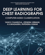
The basic architectures of CNN models are either series networks that are stacked layers in a contiguous manner or DAG networks where the output of one layer is an input to multiple layers at different levels. Fig. 4.3 shows the different types of pre-trained networks available in the MATLAB Deep Learning Toolbox where the networks shaded in gray are used in the present work.

4.4.1: Series end-to-end pre-trained CNN model: AlexNet

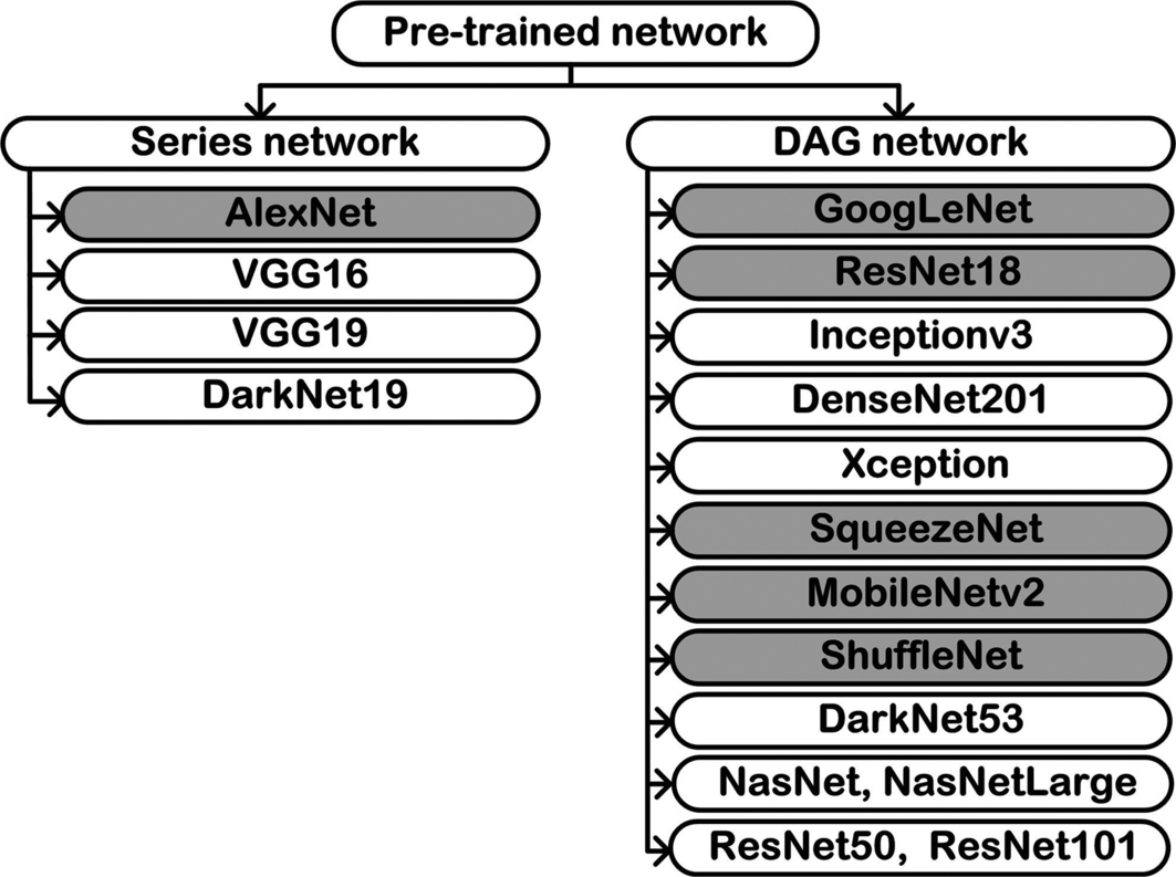
A CNN marked the breakthrough in deep learning by winning the ImageNet Large Scale Visual Recognition Challenge (ILSVRC) 2012, and it was introduced by Alex Krizhevsky et al. in the year 2012 [20]. AlexNet is a 25-layer network comprising of eight deep layers formed by convolutional layers (five layers) and fully connected layers (three layers), and the remaining layers consist of max pooling layers, normalization layers, rectified linear unit (ReLU) activation layers, and dropout layers. AlexNet was the first deep CNN to use ReLU as the activation function, which is considered to be the reason for the massive boost in the accuracy of the network. In addition to ReLU activation, Krizhevsky applied the normalization and dropout layers along with heavy data augmentation with an attempt to improve the general performance. The convolutional layers of AlexNet are of different sizes, such as 11 × 11, 5 × 5, 3 × 3, each having different strides and padding. The ReLU activation is applied after every convolutional layer followed by the normalization and the max pooling layers. Fig. 4.4 shows the basic architecture of AlexNet. The network has an input size of 227 × 227 × 3. All the layers are piled up on each other or arranged one after the other; hence, AlexNet is often referred to as a type of series network [20]. In AlexNet, each of convolutional layer aims at automatic feature extraction from the input image, whereas the source of nonlinearity in this series network is the ReLU activation function. It has been extensively used in the classification of medical images of various types [20–25].

4.4.2: Directed acyclic graph end-to-end pre-trained CNN model: ResNet18

The residual network has multiple variations, namely ResNet16, ResNet18, ResNet34, ResNet50, ResNet101, ResNet110, ResNet152, ResNet164, ResNet1202, and so forth. The ResNet stands for residual networks and was named by He et al. 2015 [26]. ResNet18 is a 72-layer architecture with 18 deep layers. The architecture of this network aimed at enabling large amounts of convolutional layers to function efficiently. However, the addition of multiple deep layers to a network often results in a degradation of the output. This is known as the problem of vanishing gradient where neural networks, while getting trained through back propagation, rely on the gradient descent, descending the loss function to find the minimizing weights. Due to the presence of multiple layers, the repeated multiplication results in the gradient becoming smaller and smaller thereby “vanishing” leading to a saturation in the network performance or even degrading the performance.

The primary idea of ResNet is the use of jumping connections that are mostly referred to as shortcut connections or identity connections. These connections primarily function by hopping over one or multiple layers forming shortcuts between these layers. The aim of introducing these shortcut connections was to resolve the predominant issue of vanishing gradient faced by deep networks. These shortcut connections remove the vanishing gradient issue by again using the activations of the previous layer. These identity mappings initially do not do anything much except skip the connections, resulting in the use of previous layer activations. This process of skipping the connection compresses the network; hence, the network learns faster. This compression of the connections is followed by expansion of the layers so that the residual part of the network could also train and explore more feature space. The input size to the network is 224 × 224 × 3, which is predefined. The network is considered to be a DAG network due to its complex layered architecture and because the layers have input from multiple layers and give output to multiple layers. Residual networks and their variants have broadly been implemented for the analysis of medical images [22, 27–29]. Fig. 4.5 shows the layer architecture of ResNet18 CNN model.

The introduction of residual blocks overcomes the problem of vanishing gradient by implementation of skip connections and identity mapping. Identity mapping has no parameters and maps the input to the output, thereby allowing the compression of the network, at first, and then exploring multiple features of the input. Fig. 4.6 shows a typical residual block used in ResNet18 CNN model.

4.4.3: DAG end-to-end pre-trained CNN model: GoogLeNet

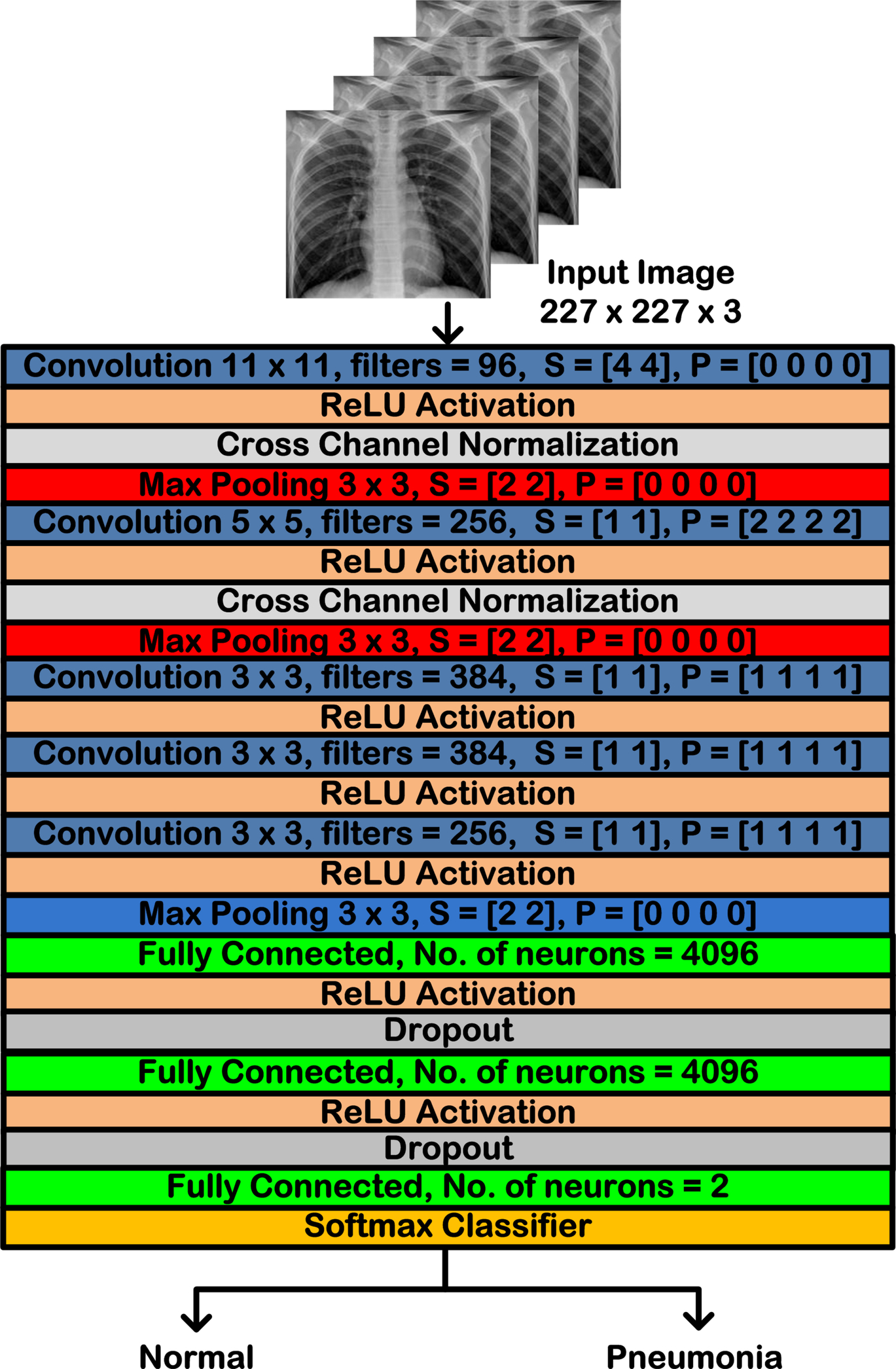
The GoogLeNet architecture was the 2014 winner of the ILSVRC and has a 144-layer architecture comprising of 22 deep layers and other pooling layers, ReLU activation layers, and dropouts, given by Szegedy et al. [30]. It is a carefully designed architecture with a deeper network to enhance the overall computational efficiency. It introduced an efficient inception module with an aim of reducing the computational complexity and the amount of parameters being utilized in the network. The GoogLeNet architecture includes the concept of bottleneck layers that are the 1 × 1 convolutions. These convolutions aim at reducing the dimensions, thereby contributing in the overall reduction of the computational bottlenecks. Another concept that enhances the performance of GoogLeNet is the replacement of fully connected layers by the global average pooling (GAP) and the inception module. The GAP layers reduce the computation cost of the network due to the absence of the trainable weights in this layer. There are nine inception modules being applied in the middle of the network. The general layer architecture of GoogLeNet and the basic configuration of an inception module are shown in Fig. 4.7.

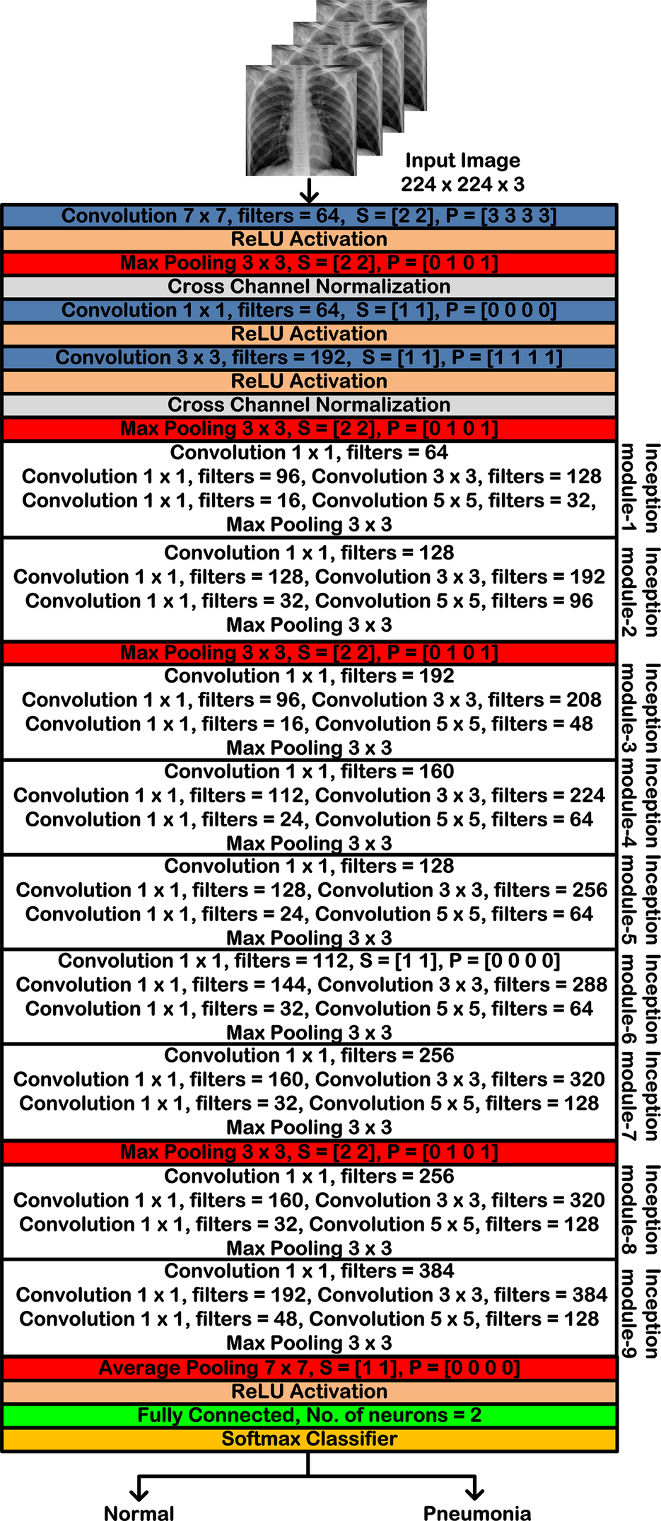
The inception network contains the grouping of all the convolutions (1 × 1, 3 × 3, 5 × 5). The final result of this combination of convolutions is the concatenation of the results of each convolution (1 × 1, 3 × 3, 5 × 5). These modules were introduced with an aim to reduce the disparity in evidence of an entity associated with the entity location in the form of information in an image. Extracting this location information often requires the selection of the appropriate kernel size since larger kernels mostly associate with extracting the information, which is distributed globally, whereas a smaller sized kernel is well-matched for the task of extracting the information that has a local distribution. The network is considered to be a DAG network due to its complex layered architecture and because the layers have input from multiple layers and give output to multiple layers. The GoogLeNet architecture has been applied broadly in the analysis of numerous medical images [31–33]. A general inception module consists of 1 × 1 convolution layers often referred to as the bottleneck layers. These 1 × 1 convolutions are introduced for dimensionality reduction in GoogLeNet. Fig. 4.8 shows an inception module used in GoogLeNet architecture.

4.5: Decision fusion

As the name suggests, decision fusion aims at combining the decisions taken by different classifiers to achieve a common consensus that is better than the individual decisions of the classifiers [34, 35]. In simple words, decision fusion is the method of combining the decisions taken by multiple classifiers to reach a common final decision. Here the decision of the classifier is the classification performed on the test dataset, which is the prediction on the test dataset. The process includes coalescing the information from different datasets or different classifiers after each data has been subjected to preliminary classification. Decision fusion is performed with an aim to enhance the performance of the classification task. Classifiers often have different classification performances depending on the type of data they are working with as well as their architecture. However, many times different classifiers have varied performance for the same classification problem. The decisions taken by a classifier are broadly of three types: (a) measurement level: this type of decision involves the classifier returning a real valued vector; (b) rank level: this type of decision involves the classifiers to return an ordered sequence of classes; and (c) abstract level: this is the most widely applied type of decision where the classifiers return a single class label as the decision. Fig. 4.9 shows the different types of decisions that can be taken by a classifier.

Fig. 4.10 shows the broad categorization of the decision fusion techniques.

On the other hand, the decision fusion techniques are broadly classified on the basis of the fusion architecture used; these include the following:

1. (a) Serial decision fusion: In this architecture, the classifiers are arranged in series; the output of one classifier acts as an input to the next. Fig. 4.11 shows the series decision fusion.

   
   

1. (b) Parallel decision fusion: In this, the classifiers are arranged in parallel and the classifiers perform classification simultaneously and then the decision fusion is performed. Fig. 4.12 shows the parallel decision fusion.

   
   

1. (c) Hybrid decision fusion: This is a hierarchical structure of classifiers. Fig. 4.13 shows the hybrid decision fusion.

   
   

On the basis of the fusion type, these techniques are of two types:

1. (a) Voting-based: In the voting-based decision fusion techniques, majority voting is the most popular and is widely used. Some of the other techniques include weighted voting in which a weight to each classifier is attached and then decision fusion is performed. Borda count is another technique in which the sums of reverse ranks are calculated to perform decision fusion [36]. Other voting techniques are probability-based, such as fuzzy rules, Naïve-Bayes, Dempster-Shafer theory, and so forth [35, 37, 38].
2. (b) Divide and conquer: In this decision fusion technique, the dataset is divided into subsets of equal sizes, and then the classification is performed followed by decision fusion on the results of those smaller dataset classifications. These divide and conquer methods include the concepts of bagging and boosting.

The present work implements the majority voting of the different CNN-based pre-trained models with a parallel architecture of the decision fusion technique.

4.6: Experiments and results

Experiment 1: Designing end-to-end pre-trained CNN-based CAC system for chest radiographs using AlexNet

In Experiment 1, the CAC system for binary class classification of chest radiograph images is designed using AlexNet CNN model. The network has been trained using the augmented chest radiograph image dataset for classification of chest radiograph images. The results of performance evaluation of the CAC system designed using AlexNet CNN for chest radiographs are shown in Table 4.1.

From the results of Experiment 1, as shown in Table 4.1, it can be seen that the CAC system designed using end-to-end pre-trained AlexNet CNN model achieves 89.00% accuracy for the classification of chest radiograph images into two classes: Normal and Pneumonia. The individual class accuracy of the Normal class is 98.00%, and for the Pneumonia class, the individual class accuracy obtained is 80.00%. From the total 100 images in the testing set, 11 images have been misclassified from which only one instance belongs to the Normal class and the remaining 10 misclassified images are of the Pneumonia class.

Code Snippet 4.1 shows the syntax of loading the training dataset. The chest X-ray images are divided and kept in three folders, namely training, validation, and testing. The training data is loaded from the path “H:DataChestxrayTraining,” which further contains two folders named as per the class labels of Normal and Pneumonia.

%%Loading the training dataset%% imds_train  =  imageDatastore('H:DataChestxrayTraining','IncludeSubfolders',true, 'LabelSource','foldernames');

Code Snippet 4.2 shows the syntax of loading the validation dataset. The validation data is loaded from the path “H:DataChestxrayValidation,” which further contains two folders named as per the class labels Normal and Pneumonia, just as those of the training dataset.

%%Loading the validation dataset%% imds_val  =  imageDatastore('H:DataChestxrayValidation','IncludeSubfolders',true, 'LabelSource','foldernames');

Code Snippet 4.3 shows the syntax of loading the testing dataset. The testing data is loaded from the path “H:DataChestxrayTesting,” which further contains two folders named as per the class labels Normal and Pneumonia, just as those of the training and validation datasets.

%%Loading the testing dataset%% imds_test  =  imageDatastore('H:DataChestxrayTesting','IncludeSubfolders',true, 'LabelSource','foldernames');

After the dataset has been loaded, the target CNN model is loaded as shown in Code Snippet 4.4. For Experiment 1, the AlexNet CNN model is used; hence, it is loaded to further proceed with the training process.

%%loading the AlexNet pre-trained CNN model%%net = alexnet;

As the target network is also loaded into the MATLAB workspace, one needs to specify the training options so as to facilitate training of the CNN model. Code Snippet 4.5 shows the training options set for Experiment 1.

%%specifying the training options %%Training_options = trainingOptions('rmsprop', 'InitialLearnRate', 0.0001, 'Plots', 'training-progress', 'ValidationData', imds_val, 'ValidationFrequency',10,'Shuffle', 'every-epoch','MaxEpochs',10, 'MiniBatchSize',45);

Code Snippet 4.6 shows the syntax of training the network using the training data and the CNN model loaded into the workspace on the previously defined training options.

%%training the CNN model%% Exp1_alexnet  = trainNetwork(imds_train,lgraph_1, Training_options);

Code Snippet 4.7 shows the syntax of projecting the test data onto the trained network. The predictions of the trained CNN model are in the form of a confusion matrix.

%%using trained network to classify images%% [predictions,prediction_score] = classify(Exp1_alexnet,imds_test);true_testing = imds_test.Labels;nnz(predictions == true_testing)/numel(predictions);[confusion_matrix, matrix_order] =confusionmat(true_testing,predictions);heatmap(matrix_order, matrix_order, confusion_matrix);accuracy = mean(predictions  ==true_testing)

Once the network is trained, it is beneficial to save the network for future reference. This can be done using the save() function as shown in Code Snippet 4.8. The results of Experiment 1 are saved in a “mat” file named 'Exp1_alexnet.mat'.

%%saving the trained AlexNet CNN model%%save('Exp1_alexnet')

Experiment 2: Designing end-to-end pre-trained CNN-based CAC system for chest radiographs using ResNet18

In Experiment 2, the CAC system for binary class classification of chest radiograph images is designed using ResNet18 CNN model. The network has been trained using the augmented chest radiograph image dataset for classification of chest radiograph images. The results of performance evaluation of the CAC system designed using ResNet18 CNN for chest radiographs are shown in Table 4.2.

From the results of Experiment 2, as shown in Table 4.3, it can be seen that the CAC system using ResNet18 CNN model gives 88.00% accuracy for the classification of chest radiograph images into two classes: Normal and Pneumonia. The individual class accuracy of the Normal class is 100.00%, and for the Pneumonia class, the individual class accuracy value obtained is 76.00%. From the total 100 images in the testing set, 12 images have been misclassified, which all belong to the Pneumonia class.

Code Snippet 4.9 shows the syntax of loading the training dataset. The chest X-ray images are divided and kept in three folders namely training, validation, and testing. The training data is loaded from the path “H:DataChestxrayTraining,” which further contains two folders named as per the class labels of Normal and Pneumonia.

%%Loading the training dataset%% imds_train  =  imageDatastore('H:DataChestxrayTraining','IncludeSubfolders',true, 'LabelSource','foldernames');

Code Snippet 4.10 shows the syntax of loading the validation dataset. The validation data is loaded from the path “H:DataChestxrayValidation,” which further contains two folders named as per the class labels Normal and Pneumonia, just as those of the training dataset.

%%Loading the validation dataset%% imds_val  =  imageDatastore('H:DataChestxrayValidation','IncludeSubfolders',true, 'LabelSource','foldernames');

Code Snippet 4.11 shows the syntax of loading the testing dataset. The testing data is loaded from the path “H:DataChestxrayTesting,” which further contains two folders named as per the class labels Normal and Pneumonia, just as those of the training and validation datasets.

%%Loading the testing dataset%% imds_test  =  imageDatastore('H:DataChestxrayTesting','IncludeSubfolders',true, 'LabelSource','foldernames');

After the dataset has been loaded, the target CNN model is loaded as shown in Code Snippet 4.12. For Experiment 2, ResNet18 CNN model is used; hence, it is loaded to further proceed with the training process.

%%loading the resnet18 pre-trained CNN model%%net = resnet18;

As the target network is also loaded into the MATLAB workspace, now one needs to specify the training options so as to facilitate training of the CNN model. Code Snippet 4.13 shows the training options set for Experiment 2.

%%specifying the training options %%Training_options = trainingOptions('rmsprop', 'InitialLearnRate', 0.0001,'Plots','training-progress','ValidationData',imds_val, 'ValidationFrequency',10,'Shuffle','every-epoch','MaxEpochs',10, 'MiniBatchSize',45);

Code Snippet 4.14 shows the syntax of training the network using the training data and the CNN model loaded into the workspace on the previously defined training options.

%%training the CNN model%% Exp2_resnet18  = trainNetwork(imds_train,lgraph_1, Training_options);

Code Snippet 4.15 shows the syntax of projecting the test data onto the trained network. The predictions of the trained CNN model are in the form of a confusion matrix.

%%using trained network to classify images%% [predictions,prediction_score] = classify(Exp2_resnet18,imds_test);true_testing = imds_test.Labels;nnz(predictions == true_testing)/numel(predictions);[confusion_matrix, matrix_order] =confusionmat(true_testing,predictions);heatmap(matrix_order, matrix_order, confusion_matrix);accuracy = mean(predictions  ==true_testing)

Once the network is trained, it is beneficial to save the network for future reference. This is done using the save() function as shown in Code Snippet 4.16. The results of Experiment 2 are saved in a “mat” file named 'Exp2_resnet18.mat'.

%%saving the trained AlexNet CNN model%%save(‘Exp2_resnet18’)

Experiment 3: Designing end-to-end pre-trained CNN-based CAC system for chest radiographs using GoogLeNet

In Experiment 3, the CAC system for binary class classification of chest radiograph images is designed using GoogLeNet CNN model. The network has been trained using the augmented chest radiograph image dataset for classification of chest radiograph images. The results of performance evaluation of CAC system designed using GoogLeNet CNN for chest radiographs are shown in Table 4.3.

From the results of Experiment 3, as shown in Table 4.3, it can be seen that the CAC system designed using GoogLeNet CNN model achieves 90% accuracy for the classification of chest radiograph images into two classes: Normal and Pneumonia. The individual class accuracy of the Normal class is 96%, and for the Pneumonia class, the individual class accuracy obtained is 84%. From the total 100 images in the testing set, 10 images have been misclassified, out of which 2 belong to the Normal class and 8 belong to the Pneumonia class.

Code Snippet 4.17 shows the syntax of loading the training dataset. The chest X-ray images are divided and kept in three folders, namely training, validation, and testing. The training data is loaded from the path “H:DataChestxrayTraining,” which further contains two folders named as per the class labels of Normal and Pneumonia.

%%Loading the training dataset%% imds_train  =  imageDatastore('H:DataChestxrayTraining','IncludeSubfolders',true, 'LabelSource','foldernames');

Code Snippet 4.18 shows the syntax of loading the validation dataset. The validation data is loaded from the path “H:DataChestxrayValidation,” which further contains two folders named as per the class labels Normal and Pneumonia, just as those of the training dataset.

%%Loading the validation dataset%% imds_val  =  imageDatastore('H:DataChestxrayValidation','IncludeSubfolders',true,'LabelSource','foldernames');

Code Snippet 4.19 shows the syntax of loading the testing dataset. The testing data is loaded from the path “H:DataChestxrayTesting,” which further contains two folders named as per the class labels Normal and Pneumonia, just as those of the training and validation datasets.

%%Loading the testing dataset%% imds_test  =  imageDatastore('H:DataChestxrayTesting','IncludeSubfolders',true, 'LabelSource','foldernames');

After the dataset has been loaded, the target CNN model is loaded as shown in Code Snippet 4.20. For Experiment 3, GoogLeNet CNN model is used; hence, it is loaded to further proceed with the training process.

%%loading the GoogLeNet pre-trained CNN model%%net = googlenet;

As the target network is also loaded into the MATLAB workspace, now one needs to specify the training options so as to facilitate training of the CNN model. Code Snippet 4.21 shows the training options set for Experiment 3.

%%specifying the training options %%Training_options = trainingOptions('sgdm', 'InitialLearnRate', 0.0001, 'Plots', 'training-progress', 'ValidationData', imds_val, 'ValidationFrequency',10,'Shuffle','every-epoch','MaxEpochs',10, 'MiniBatchSize',45);

Code Snippet 4.22 shows the syntax of training the network using the training data, and the CNN model is loaded into the workspace on the previously defined training options.

%%training the CNN model%% Exp3_GoogLeNet  = trainNetwork(imds_train,lgraph_1,Training_options);

Code Snippet 4.23 shows the syntax of projecting the test data onto the trained network. The predictions of the trained CNN model are in the form of a confusion matrix.

%%using trained network to classify images%% [predictions,prediction_score] = classify(Exp3_GoogLeNet,imds_test);true_testing = imds_test.Labels;nnz(predictions == true_testing)/numel(predictions);[confusion_matrix, matrix_order] = confusionmat(true_testing,predictions);heatmap(matrix_order, matrix_order, confusion_matrix);accuracy = mean(predictions  ==true_testing)

Once the network is trained, it is beneficial to save the network for future reference. This is done using the save() function as shown in Code Snippet 4.24. The results of Experiment 3 are saved in a “mat” file named 'Exp3_GoogLeNet.mat'.

Experiment 4: Designing end-to-end pre-trained CNN-based CAC system for chest radiographs using decision fusion

In Experiment 4, the CAC system for binary class classification of chest radiograph images is designed using decision fusion of the pre-trained CNN models that have been trained using the augmented chest radiograph image dataset for classification of chest radiograph images in Experiments 1–3. The results of performance evaluation of the CAC system designed using decision fusion for binary classification of chest radiographs are shown in Table 4.4.

From the results of Experiment 4, as shown in Table 4.4, it can be seen that the CAC system designed using the decision fusion of the CNN models in Experiments 1–3 achieves 91.00% accuracy for the classification of chest radiograph images into two classes of Normal and Pneumonia. The individual class accuracy of the Normal class is 100.00%, and for the Pneumonia class, the individual class accuracy obtained is 82.00%. From the total 100 images in the testing set, 9 images have been misclassified, which all belong to the Pneumonia class. The ROC curve with its corresponding AUC values for the CAC system designed using the different CNN models is shown in Fig. 4.14.

4.7: Concluding remarks

From the assessment of the experiments carried out in this chapter to evaluate the performance of the popularly used CNN networks AlexNet, ResNet-18, and GoogLeNet and on the basis of the results obtained from the experiments carried out in the present work, it is observed that GoogLeNet CNN model performs best for the classification of chest radiographs.

A comparative analysis of the obtained results from the experiments carried with different CNN models for the classification of chest radiographs is given in Table 4.5.

Therefore, for further analysis of the performance of machine learning-based classifiers, the GoogLeNet CNN model is used for deep feature extraction. The subsequent chapters deal with the design of a CAC system for chest radiographs using deep feature extraction, GoogLeNet, ANFC-LH classifier, and PCA-SVM classifier.