Chapter 3: Methodology adopted for designing of computer-aided classification systems for chest radiographs
Abstract
This chapter describes the methodology adopted for the present work. A brief overview of the CAC system for chest radiographs designed in this book are given as well as a general overview to the need for CAC systems, specifically for chest radiographs, and the importance of CAC systems in current scenarios due to the wide spread of COVID-19. The different approaches of designing CAC systems have been discussed with respect to the type of CNN used and the number of output classes. The chapter describes the dataset used for designing the CAC systems, the different augmentation techniques, and the motivation for dataset augmentation. The implementation details discussed include the hardware and software requirements, installing the Deep Learning Toolbox, the various hyperparameters that play important roles in learning of a deep learning model. The code snippets of data augmentation and image resizing, aimed at giving a better understanding of the programmatic implementation of these processes.
Keywords
Computer-aided classification; CAC system designs; Data augmentation; Kaggle chest X-Ray dataset; Hyperparameters; Batch; Epoch; Learning rate; Activation function; Deep Learning Toolbox
3.1: Introduction
In this chapter a brief overview of the computer-aided classification (CAC) system for chest radiographs designed in this book are given as well as a general overview to the need for CAC systems specifically for chest radiographs, the importance of CAC systems in current scenarios due to the wide spread of COVID-19. The different approaches of designing CAC systems have been discussed with respect to the type of convolution neural network (CNN) used and the number of output classes. This chapter describes the dataset used for designing the CAC systems, the different augmentation techniques, and the motivation for dataset augmentation. The implementation details discussed include the hardware and software requirements, installing the Deep Learning Toolbox, and the various hyperparameters such as the activation function, epoch, batch size, learning rate, optimizer, and so on that play an important role in learning of a deep learning-based model. The code snippets of the different augmentation techniques aim at giving a better understanding to the programmatic implementation of data augmentation, specifically for chest radiographs.
3.2: What is a CAC system?
A CAC system, as the name suggests, is a computer-based system that facilitates the medical practitioners to take decisions quickly and more efficiently. The medical images have immense amounts of data that the doctors need to assess and evaluate in order to determine the presence of an abnormality. This process is time-consuming whereas the medical practitioners intend at performing the same task in a short span so that timely diagnosis could lead to timely treatment thereby saving the life of critical patients. A CAC system with a purpose to detect abnormalities in medical images includes multiple components such as preprocessing of the input of medical images, the segmentation of the region of interest (ROI), feature extraction, and classification. It is not mandatory that all CAC system designs include every component discussed. The components of any computer-aided system depend on the task they are being designed for. A segmentation-based computer-aided system would focus on segmentation of the ROI whereas a classification-based computer-aided system may or may not perform segmentation. Fig. 3.1 shows some of the basic components of a CAC system.

3.3: Need for CAC systems
CAC systems in medical imaging have flourished immensely over the span of several years. Ever-improving software as well as hardware specifications and the advancements in the quality of imaging modalities have contributed to the successful design of these CAC systems. Some of the major reasons for the increase in need for CAC systems can be stated as follows:
- • Overcome observational oversights: One of the major driving forces for the increased need for CAC systems is the aim to overcome observational oversights of the medical practitioners and surpass the limitations of human observers in interpreting medical images.
- • Reduce error in medical image interpretation: Another limitation is the error and false negative as well as false positive rates of screening different medical images. Hence CAC systems aim at reducing the errors that are not possible to handle at a human end.
- • Increase in detection of diseases: For disease detection, different medical imaging modalities are used. Each disease has its own characteristic features that are essential for correct diagnosis. However, some of these features may be missed by the human eye. Here the mathematical descriptors are capable of detecting and carefully analyzing these features. This plays an important role in efficient and early diagnosis of diseases.
- • Double reading: CAC systems often reduce the concept of double reading by another medical practitioner, which is nothing but consulting another radiologist for a second opinion or confirmation on the observation done by the first radiologist. Here CAC systems can reduce the need for double readings.
Although CAC systems cannot substitute medical practitioners, they can ease their work by helping them in becoming better decision makers.
3.4: Need for CAC systems for chest radiographs
The differential diagnosis of chest radiographs is a challenging task even for experienced and skilled radiologists. The appearance of both pneumonia and COVID-19 on a chest radiograph is similar (cloudy appearance or ground glass opacity), and it is difficult for even an experienced radiologist to distinguish between them by simply looking at a chest radiograph. Since COVID-19 is a recent pandemic on which multiple studies are still being conducted with an aim to improve the diagnosis and analyze the key features that can play vital roles in distinguishing COVID-19 from pneumonia. However, the features that are not distinguishable to naked human eye can be easily detected by the mathematical descriptors.
Therefore, there lies significant motivation among the community of researchers with an aim to develop and improve the quality of CAC systems for differential diagnosis between chest radiographs. Some of the major reasons CAC systems are needed for chest radiographs can be stated as follows:
- • Overcome complexity of interpretation of chest radiographs: The chest radiographs provide immense amounts of information about the health of a patient. Overlying tissues increase the complexity of radiographs making it difficult for medical practitioners to interpret such visually complex information correctly and precisely. This often leads to misdetection and misdiagnosis of diseases even by the most experienced and skilled radiologists. In some cases the contrast between the lesions and the surrounding area is so low that it is invisible to the naked human eye; however, these minor contrast changes can be efficiently detected by mathematical algorithms and descriptors.
- • Similar appearance of pneumonia and COVID-19 on a chest radiograph: Both pneumonia and COVID-19 appear similar when observed on a chest radiograph even to an experienced radiologist. Both have a cloudy appearance often referred to as ground glass opacity and is commonly called the hazy lung region. Since COVID-19 is spreading worldwide at an immense rate and is a dangerous disease, efficient and early detection plays vital role. Here the CAC systems designed using various machine learning and deep learning algorithms can be highly beneficial.
- • Need of the hour: The rate at which COVID-19 is spreading and the medium through which it spreads makes it a highly perilous disease. It can be transmitted through droplets in the air or on surfaces, coughing, sneezing, and so forth. Studies are still being carried out to determine the significant features so that the radiologists can correctly diagnose and differentiate between pneumonia and COVID-19 by looking at chest radiographs or CT images. Here CAC systems can be designed and trained on the limited dataset available to help in correctly diagnosing and differentiating between the diseases based on the features extracted by the mathematical descriptors from the chest radiographs that are not visible to the radiologists.
3.5: Types of classifier designs for CAC systems
Computer-aided detection and CAC are often referred to as two different terms where detection focuses on pattern recognition, identifying charts, and guarded features that are not visible to the human eye with an aim to assist radiologists in reducing misdiagnosis, whereas the term computer-aided classification includes all the tasks performed by computer-aided detection with an additional task of predicting the likelihood of a feature that represents a particular disease.
The main aim of any CAC system design is to improve the interpretation of images with significantly reduced amounts of error. The development of CAC systems is not an easy task as the best results are obtained through the analysis carried out by the medical practitioners in real time. Obtaining the reference standard of the truth is highly labor intensive and requires an immense amount of effort in data collection and massive investment of time. Different researchers propose different methodologies for designing CAC systems; however, there is no one specific foolproof design paradigm. Some of the common approaches used to design CAC systems are discussed in this section. Fig. 3.2 shows the different types of approaches to designing classifiers for CAC system, the classifier designs in gray are used in the present work.

3.5.1: On the basis of number output classes
CAC systems can be designed on the basis of the numbers of output classes or the number of classes in which the data is divided into and labeled for the task of supervised classification.
- (a) Binary classifier: This type of CAC system deals with binary class classification of the images, such as benign/malignant or Normal/Abnormal [1–17]. In the present work the CAC systems are designed based on this approach focusing on the classification of chest radiographs into Normal and Pneumonia. Fig. 3.3 shows the schematic representation of different binary class classifiers.

Fig. 3.3 Schematic representation of types of binary classifier.
- (b) Multiclass classifier: These types of CAC system designs have more than two class labels. The class labels represent the number of output classes. This can either be a simple three-class classifier dealing with three classifications of the input data or it could be a hierarchical structure. The broad division of a multiclass classifier is discussed as follows:
- (i) Single three-class classifier: This type of CAC systems deals with a simple three-class classification of the images, such as Normal, Pneumonia, and COVID-19 for chest radiographs [9, 18–22]. Fig. 3.4 shows the schematic representation of a simple three-class classifier.

Fig. 3.4 Schematic representation of a three-class classifier. - (ii) Hierarchical classifier: This type of CAC system design first classifies the images into some classes and then further classifies them into subclasses, such as the classification of chest radiographs into Normal/Abnormal then further classifying Abnormal images into Pneumonia/COVID-19. Fig. 3.5 is a schematic representation of a hierarchical classifier where the classifier 1 and classifier 2 can be either a machine learning-based or a deep learning-based classifier.

Fig. 3.5 Schematic representation of a hierarchical classifier.
- (i) Single three-class classifier: This type of CAC systems deals with a simple three-class classification of the images, such as Normal, Pneumonia, and COVID-19 for chest radiographs [9, 18–22]. Fig. 3.4 shows the schematic representation of a simple three-class classifier.
3.5.2: On the basis of learning approach
CAC systems are designed with an aim to search for the same features that a radiologist would look for in a medical image to perform the diagnosis. Each disease has its own unique identifiers that enable the radiologists to correctly diagnose it, such as for diagnosis of pneumonia the radiologist looks at chest radiographs to find opacity of the lungs and see pulmonary densities. For other lung-related diseases features such as sphericity of the lung nodules are searched for [23–29]. Similarly for breast cancer the radiologist looks at mammograms or ultrasound images of breasts for features such as spiculated mass, nonspiculated mass distortion, micro-calcifications, and asymmetries [25, 30, 31]. All of these features can sometimes be unclear or invisible to the human eye, and here various mathematical algorithms play a vital role. These mathematical descriptors or algorithms can identify even minor differences in the images and therefore are highly useful in such cases.
The most popular CAC system design learning approaches are machine learning-based algorithms and deep learning-based algorithms. Both of the approaches are discussed here.
- (a) Machine learning: This learning approach is used where the features of the images can be manually mined and fed to the algorithm [32–34]. The machine learning methods are of three types:
- (i) Supervised learning: For supervised learning the training data has well-labeled outputs for their corresponding input values. This method aims at mapping a mathematical relationship between the input and the well-labeled output. The output data has categorical values in case of classification tasks and continuous numerical values in case of regression tasks; depending on the task, the output data value type changes. Some supervised machine learning algorithms are k-NN and support vector machines (SVMs). [35–37].
- (ii) Unsupervised learning: In unsupervised learning the labeled outputs are not available. This learning method determines a functional representation of the hidden characteristics of the input data. Some unsupervised machine learning algorithms are PCA and cluster analysis [34, 38–45].
- (iii) Reinforcement learning: Reinforcement learning is primarily concerned with sequential decision problems. It is not popularly used in medical imaging-related problems and tasks as it learns by trial and error and has a tendency to affect future patient treatments with bias [46, 47].
The machine learning approach is not used for the design of chest radiographs since they depend greatly on the handcrafted features by the experts. This manual extraction of features is not optimal, as the data varies from patient to patient and sometimes many of the otherwise highly useful features for classification are lost.
- (b) Deep learning: The deep learning approach is more reliable as compared to machine learning algorithms as it offers automatic feature extraction, and the labor intensive work of manual feature extraction is no more a concern. It is a subsidiary of supervised machine learning algorithms but is most effective and has proven to give promising results [48–52].
A branch of machine learning that primarily deals in processing data, trying to mimic the thinking process and develop abstractions by employing algorithms, is often defined as deep learning. It makes the use of multiple layers of algorithms with an aim to process the data, understanding human speech, and recognize objects visually. The most popularly known algorithms are the CNN and the deep convolution neural network (DCNN). The collected information passes through each layer of the network satisfying the temporal dependencies by serving the results of the previous layer as an input to the succeeding layer. The very first layer of the network is known as the input layer, whereas the last layer provides the output; hence, it is called the output layer. The layers in between the input and the output are known as hidden layers. Each layer can be defined by an identical, uniform, and unvarying algorithm that simply implements similar kinds of activation functions. An additional popular and most important trait of deep learning is the technique of feature extraction. This is done by using various algorithms to extract the features automatically with an aim to build a significant set of features of the input data essentially for the purpose of training the neural networks or deep networks as well as facilitating efficient and meaningful learning.
In the present work for the design of CAC systems for chest radiographs, the deep learning-based approach is chosen as it can extract those features from the X-ray images that are not visible to the human eye.
3.6: Deep learning-based CAC system design
As previously discussed, chest radiographs provide radiologists with huge amounts of information and this information varies from patient to patient, which is sometimes difficult to process manually. Therefore, a deep learning-based approach helps by automating feature extraction and learning those features to perform correct diagnoses. Deep learning-based CAC systems are discussed in this chapter, and the schematic representation of the broad distribution is shown in Fig. 3.6.

3.6.1: On the basis of network connection
- (a) Series network: In a series network all the layers forming the network are piled up on each other and arranged one after the other in a contiguous manner. Each layer has an input only from its immediate previous layer and gives output to only its immediate next layer. Here each layer has access parameters of only two layers. Some of the series CNN models are AlexNet, VGG16, VGG19, and DarkNet. Fig. 3.7 gives a schematic representation of series network.

Fig. 3.7 Schematic representation of series network.
- (b) DAG network: The DAG network stands for Directed Acyclic Graphs as the arrangement of the layers of the network is similar to directed acyclic graphs. These networks have directed connections to multiple layers. The layers of the network have input from multiple layers and gives output to multiple layers. Some of the DAG networks are SqueezeNet, GoogLeNet, ResNet50, ResNet101, ResNet18, InceptionV3, DenseNet201, NASNet-Large, and NASNet-Mobile. Fig. 3.8 gives a schematic representation of a DAG network.

Fig. 3.8 Schematic representation of a DAG network.
3.6.2: On the basis of network architecture
- (a) End-to-end CNN: This type of CAC system is designed by using a single CNN model that can specialize in predicting the output from the inputs. This often results in the development of a complex state-of-the-art system. These end-to-end systems (E2E systems) are very expensive; hence, many industries are unenthusiastic about their use and application. The primary idea of utilizing a single CNN model for performing a specific task has multiple obstacles such as requirement of enormous amounts of training data, inefficient training, and difficulties in performing validation of the CAC system designed. Another major drawback faced while designing the E2E CAC systems is that in worst-case scenarios the network might not learn at all, hence training such systems is inefficient and dicey. Fig. 3.9 shows an E2E CNN-based CAC system design.

Fig. 3.9 Schematic representation of end-to-end CNN-based CAC.
- (b) Lightweight E2E CNN: Lightweight network architecture has certain properties that are highly desirable: the maximized use of balanced convolutions preferably equivalent to the channel width; analyze the cost of convolutions and the combinations being used; the reduction of degree of fragmentation; and the decrease in the number of element-wise operations. All of these properties combined results in the overall reduction of memory use and an immense increase in processing time. Some of the lightweight CNN models include SqueezeNet, ShuffleNet, MobileNetV2, and NASNet. Fig. 3.10 shows a lightweight E2E CNN-based CAC system design.
Fig. 3.10 Schematic representation of a lightweight end-to-end CNN-based CAC system.
- (c) Self-designed CNN: As the name suggests, the CAC systems are designed using the CNN that have been designed by the researcher themselves.
- (d) Hybrid CNN: The idea behind hybrid CNN-based CAC system is to use machine learning classifiers for performing predictions on the input data. The aim is to use CNN for automatic feature extraction and then feed these deep feature sets to the machine learning classifiers to perform prediction or classification. Another approach is the fusion of the CNN-based deep features and the handcrafted feature from the input data, then feeding this combination to the machine learning classifier. Some of the popularly used machine learning classifiers in hybrid systems are SVMs. The present work also focuses on designing hybrid CAC systems for chest radiographs where the E2e CNN are used as deep feature extractors and then PCA-SVM, ANFC-LH like machine learning algorithms are used to perform the differential binary classification. Fig. 3.11 shows a hybrid CAC system design.

Fig. 3.11 Schematic representation of hybrid CAC: (A) CNN as deep feature extractor; (B) CNN as deep feature extractor and feature fusion with handcrafted features.
3.7: Workflow adopted in the present work
CAC system designs can be broadly considered of two types: (a) CNN-based CAC system designs, which includes the design of CAC systems using different series and DAG networks as well as lightweight CNN models; and (b) CNN-based CAC systems using deep feature extraction, which includes the CAC system design using the series and DAG networks as deep feature extractors and then applying the machine learning classifiers PCA-SVM and ANFC-LH.
The schematic representation of the workflow adopted in the present work is shown in Fig. 3.12. The workflow primarily includes the dataset generation, which is described in detail further in this chapter, followed by the various experiments conducted to design different CNN-based CAC systems explained in detail in the upcoming chapters.

The experiments have been conducted using a comprehensive image dataset of 200 chest radiographs with cases of the image classes: Normal and Pneumonia. The image database comprises of 100 Normal chest radiographs and 100 Pneumonia chest radiographs. Further bifurcation of the dataset is described further in this chapter. The present work focuses on the design of CAC systems for the efficient diagnosis of pneumonia using chest radiographs, which includes the foremost step of dataset generation. The schematic representation of the dataset generated to be used in the design of the CAC systems is shown in Fig. 3.13.

The main task of CAC system design in the present work includes the following experiments: (a) designing CNN-based CAC systems for chest radiographs using AlexNet, ResNet-18, and GoogLeNet to identify the best performing CNN model; (b) designing a hybrid CAC system for chest radiographs using the CNN model with best performance, deep feature extraction, and ANFC-LH classifier; (c) designing a CAC system for chest radiographs using the CNN model with best performance, deep feature extraction, and PCA-SVM classifier, (d) designing lightweight CNN-based CAC systems for chest radiographs using SqueezeNet. ShuffleNet, and MobileNetV2 to identify the best performing lightweight CNN model; (e) designing a CAC system for chest radiographs using the lightweight CNN model with best performance, deep feature extraction, and ANFC-LH classifier; (f) designing a hybrid CAC system for chest radiographs using the lightweight CNN model with best performance, deep feature extraction, and PCA-SVM classifier. These can be briefly described as follows:
- (a) Designing CNN-based CAC systems for chest radiographs using AlexNet, ResNet-18 and GoogLeNet to identify the best performing CNN model: This CAC system design constitutes the first four experiments discussed in detail in Chapter 4. It deals with training the AlexNet, ResNet18, and GoogLeNet CNN models in the transfer learning mode as well as the decision fusion technique for the binary classification of chest radiographs into Normal and Pneumonia class. The CNN model with best performance is then used further in (b) and (c) as a deep feature extractor, which is discussed in detail in Chapters 5 and 6, respectively.
Fig. 3.14 shows the schematic representation of the CNN-based CAC system design for classification of chest radiographs by training AlexNet, GoogLeNet, and ResNet18 to identify the best performing CNN model.

On the basis of the experiments conducted for training the CNN models to design the CAC systems, it is concluded that the GoogLeNet CNN model performs best for the binary classification of chest radiographs with 90.00% accuracy. This GoogLeNet CNN model further acts as a deep feature extractor and is used for designing the CAC system with different machine learning classifiers in (b) and (c).
- (b) Designing a CAC system for chest radiographs using the CNN model with best performance, deep feature extraction and ANFC-LH classifier: This CAC system design is the fifth experiment and is discussed in detail in Chapter 5. It deals with using the CNN model with best performance from (a) as a deep feature extractor and then performing the binary classification of the chest radiographs using the ANFC-LH classifier.
Fig. 3.15 shows the schematic representation of designing a CAC system for deep feature extraction using the CNN model with best performance and ANFC-LH machine learning classifier.

On the basis of the experiments conducted in (a), the GoogLeNet CNN model is the best performing CNN for the classification of chest radiographs. Therefore it is used as a deep feature extractor that forms a deep feature set (DFS), which is the input for the feature selection using the correlation-based feature selection technique. This results in a feature set with a limited number of relevant features called the reduced feature set (RFS), which is additionally subjected to ANFC-LH-based feature selection to further reduce the feature set to the minimum and most relevant features. The resultant optimal feature set (OFS) is projected to the neuro-fuzzy classifier called the ANFC classifier. The CAC system designed yields 93.00% accuracy for the two-class classification of chest radiographs.
- (c) Designing a CAC system for chest radiographs using the CNN model with best performance, deep feature extraction, and PCA-SVM classifier: This CAC system design forms the sixth experiment and is discussed in detail in Chapter 6. It deals with using the CNN model with best performance from (a) as a deep feature extractor and then performing the binary classification of the chest radiographs using the PCA-SVM classifier.
Fig. 3.16 shows the schematic representation of designing a CAC system for deep feature extraction using the CNN model with best performance and PCA-SVM.

On the basis of the experiments conducted in (a), the GoogLeNet CNN model is the best performing CNN for the classification of chest radiographs. Therefore, it is used as a deep feature extractor that forms a DFS that is the input for the correlation-based feature selection followed by feature dimensionality reduction by PCA. The resultant feature set is projected to the SVM classifier. The CAC system designed yields 91.00% accuracy for the binary class classification of chest radiographs.
- (d) Designing a lightweight CNN -based CAC system for chest radiographs using SqueezeNet, ShuffleNet and MobileNetV2 to identify the best performing lightweight CNN model: This CAC system design constitutes the seventh to tenth experiment and is discussed in detail in Chapter 7. It deals with training SqueezeNet, ShuffleNet, and MobileNetV2 lightweight CNN models in the transfer learning mode as well as decision fusion technique for the binary classification of chest radiographs into Normal and Pneumonia class. The best performing lightweight CNN model is then used further in (e) and (f) as a deep feature extractor.
Fig. 3.17 shows the schematic representation of a lightweight CNN-based CAC system design for classification of chest radiographs by training SqueezeNet, ShuffleNet, and MobleNetV2 to identify the best performing lightweight CNN model.

On the basis of experiments conducted for training the lightweight CNN models to design the CAC systems it is concluded that the MobileNetV2 lightweight CNN model performs best for the binary classification of chest radiographs into Normal and Pneumonia class with 94.00%. This lightweight MobileNetV2 CNN model further acts as a deep feature extractor for (e) and (f) to design CAC systems using different machine learning-based classifiers.
- (e) Designing a hybrid CAC system for chest radiographs using the lightweight CNN model with best performance, deep feature extraction, and ANFC-LH classifier: This CAC system design is the 11th experiment and is discussed in detail in Chapter 8. It deals with using the lightweight MobileNetV2 CNN model from (d) as a deep feature extractor and then performing the binary classification of the chest radiographs using the ANFC-LH classifier.
Fig. 3.18 shows the schematic representation of designing a CAC system for deep feature extraction using the lightweight MobileNetV2 CNN model and ANFC-LH classifier.

On the basis of the experiment carried out in (d), the lightweight MobileNetV2 CNN model acts as a deep feature extractor to design a CAC system using the ANFC-LH classifier. The DFS is formed by the MobileNetV2 CNN model, which on application of CFS forms the RFS. This RFS acts as an input to the feature selection performed by ANFC-LH resulting in an OFS. The binary classification of chest radiographs is performed by the ANFC classifier and yields 95.00% accuracy.
- (f) Designing a CAC system for chest radiographs using the lightweight CNN model with best performance, deep feature extraction, and PCA-SVM classifier: This CAC system design is the final experiment and is discussed in detail in Chapter 9. It deals with using the lightweight MobileNetV2 CNN model from (d) as a deep feature extractor and then performing the binary classification of the chest radiographs using the PCA-SVM classifier.
Fig. 3.19 shows the schematic representation of designing a CAC system for deep feature extraction using the lightweight MobileNetV2 CNN model and PCA-SVM.

On the basis of the experiment carried out in (d), the lightweight MobileNetV2 CNN model acts as a deep feature extractor to design a CAC system using the SVM classifier. The DFS is formed by the MobileNetV2 CNN model, which on application of CFS forms the RFS. This RFS acts as an input for feature dimensionality reduction performed by PCA. The binary classification of chest radiographs is performed by the SVM classifier and yields 95.00% accuracy.
3.8: Implementation details
This includes a description of the hardware and software requirements for carrying out the present work.
3.8.1: Hardware and software specifications
The present work has been implemented on an HP Z4G4 PC functioning on a Windows operating system with Intel Xeon W-series, octa-core processor, NVIDIA Quadro P620 2GB GPU. The system has a 2TB hard drive with 128 GB RAM. The software used for the successful implementation of the present work was MATLABR2020a and the MATLAB Deep Learning Toolbox.
3.8.2: MATLAB Deep Learning Toolbox
The MATLAB Deep Learning Toolbox offers a framework that enables the users to implement deep neural networks, Pre-trained networks, and different deep learning-based algorithms. This toolbox offers various built-in features to make the implementation of deep learning efficient. After installing this toolbox, one can easily implement CNNs, time-series based deep networks, GAN networks, and more. It offers easy design of deep neural networks by using the network designer application called the Deep Network Designer. Another important feature is the downloading of packages to implement Pre-trained networks. Installing MATLAB automatically installs the Deep Learning Toolbox; in the event it does not install automatically, one can install it manually by following some simple steps. The steps for installation of Deep Learning Toolbox are as follows:
- Step 1: Open the MATLABR2020a application installed on your system.
- Step 2: Go to the Add-On Explorer. Fig. 3.20 shows the “Add-On Explorer” symbol in the MATLABR2020a task bar.

Fig. 3.20 Screenshot showing the Add-On Explorer.
- Step 3: Search for “Deep Learning Toolbox.” Fig. 3.21 shows the search bar of MATLABR2020a.

Fig. 3.21 Screenshot showing the search for the Deep Learning Toolbox.
- Step 4: Download and install the Deep Learning Toolbox by MathWorks. Fig. 3.22 shows the installed Deep Learning Toolbox in MATLABR2020a.

Fig. 3.22 Screenshot showing the successful install of Deep Learning Toolbox.
In case of any problems in following these steps, then one can search in the “Search documentation” tab or the Help tab to obtain instructions on how to install and use the required packages and toolboxes. MATLAB provides detailed documentation that can be accessed by anyone and are just a search away.
3.8.3: Installing Pre-trained networks
The present work uses the Pre-trained series and DAG networks for designing the CAC systems. In order to use these Pre-trained deep neural networks, their packages need to be installed separately. The generalized steps to install a Pre-trained CNN are given as follows:
- Step 1: Open the MATLABR2020a application installed on your system.
- Step 2: Go to the Add-On Explorer as shown previously while installing the Deep Learning Toolbox.
- Step 3: Search for the Pre-trained network you wish to install and use.
- Step 4: Download and install the network package provided by the MathWorks Deep Learning Toolbox Team.
Example: The steps to download Pre-trained AlexNet CNN model is as follows:
- Step 1: Open the MATLABR2020a application installed on your system.
- Step 2: Go to the Add-On Explorer.
- Step 3: Search for “AlexNet.” Fig. 3.23 shows the search bar of MATLABR2020a to search for AlexNet CNN model.

Fig. 3.23 Screenshot showing the search for Pre-trained AlexNet CNN model.
- Step 4: Download and install the network package provided by the MathWorks Deep Learning Toolbox Team titled “Deep Learning Toolbox Model for AlexNet Network by MathWorks Deep Learning Toolbox Team.” Fig. 3.24 shows the installed AlexNet CNN model in MATLABR2020a.

Fig. 3.24 Screenshot showing the successful download of Pre-trained AlexNet CNN model.
You can check whether the network package has been successfully installed or not by typing the Pre-trained network name in the command window of MATLAB2020a. If the network has been installed successfully, it shows the details of the network architecture. Otherwise, it shows a prompt to go to the Add-On Explorer to install the package. One can install the package by following the steps or through the command window. After installing all the packages, you are ready to implement your work on MATLAB2020a. Fig. 3.25 shows how one can check whether the model is installed through command prompt of MATLABR2020a.

3.8.4: Key hyperparameters of deep learning-based networks
A hyperparameter is defined as a configuration that cannot be estimated from the data. It is to be specified by the user prior to training the network. Since the best value of hyperparameters are not known, one has to iterate through a large number of combinations. These trials may result in application of rule of thumb or brute force methods to gain the values of hyperparameters that give best results. The key hyperparameters of deep learning-based networks include the learning rate, activation function, epochs, batch size, and number of hidden layers [53]. Fig. 3.26 shows the key hyperparameters.
Some of the hyperparameters that are crucial in training a network are discussed as follows:
- (a) Batch size
The batch size is simply defined as the numbers of data samples that have to be processed before the internal network parameters get updated. In other words, the number of training samples present in a single (forward + backward pass). Another approach of understanding a batch size is to consider it analogous to a for-loop that is iterating over a single sample or multiple samples and making predictions. At the end of each batch, the predictions are compared with the expected outputs and an error is calculated. This error is back-propagated to update the model parameters and improve the predictions. A training dataset is divided into one or more batches depending on the total number of training samples. Each batch is sometimes called a mini-batch.
The batch size is a carefully chosen numerical value that can evenly divide the training dataset into multiple batches of same size. Selection of the batch size in such a way makes sure that no training sample is left, the batches do not have uneven number of samples, and the network is trained efficiently without any bias.
Example: If a dataset has 10,000 images that have been split into mini-batches of size 1000 images each, then the total number of batches is 10.
The batch size is of three types depending on the number of samples in each batch:
- (i) Batch gradient descent: When the entire training dataset forms one single batch, the learning algorithm is called batch gradient descent.
Batch size = All the training samples
- (ii) Stochastic gradient descent: When the batch is the size of one sample, the learning algorithm is called stochastic gradient descent.
Batch size = 1
- (iii) Mini-batch gradient descent: When the batch size is more than one and less than the size of the training dataset, the learning algorithm is called mini-batch gradient descent.
(Batch size > 1) & (Batch size < All the training samples)
What if the training dataset is not evenly divisible by the batch size?
This does happen very often when training a deep learning model. It simply means that either the final batch has fewer samples than the other batches or some of the data samples are left and thereby not contributing to the process of training the network. To overcome this one can do the following:
- Case 1: Final batch has fewer samples: In this scenario where the final batch has fewer samples as compared to other batches, one must change the batch size to a number that evenly divides the entire dataset to equal-sized batches or add more samples using the data augmentation techniques.
- Case 2: Some samples are unused: In this scenario one can remove some samples from the dataset manually to match the batch size, add more samples using data augmentation, or change the batch size as in Case 1.
Often choosing a very large batch size results in the division of the training dataset into less batches, which is not optimal as the network may not attain generalization and might be poorly trained. On the other hand, choosing a very small batch size would result in too many batches and consume resources, such as time and memory. Both of these situations are not desirable; therefore, the batch size should be selected with utmost precision and care.
- (b) Epoch
An epoch is defined as the number of times the entire dataset passes through the network and has the opportunity to update the network parameters. The number of epochs is another important hyperparameter that determines the number of times that the learning algorithm will work through the entire training dataset. One can consider an epoch analogous to for-loop that iterates over the batch size. The number of epochs is often chosen in a multiple of 10 to ease the plotting of line plots for the training progress. These line plots have the x-axis as the number of epochs and the y-axis as the training error or loss. These plots tend to hint at whether the network is overfitting, underfitting, or suitably fit for the desired task. Unlike batch size, the number of epochs can vary from one to infinity. One can run the algorithm for as long as desired and can also stop it as desired or using some criteria such as early-stopping (when there is no change in learning or a lack of change).
- (c) Iteration
Iteration is defined as the number of times the parameters of the algorithm are updated. Here a single iteration is the number of passes that result in the gradient update. Each pass consists of the forward propagation of weights/input and backward propagation of error. The iterations are equivalent to the number of mini-batches. The completion of these iterations results in the finishing of a single epoch only.
Example: If a dataset has 10,000 images that have been split into mini-batches of size 1000 image each, then it takes 10 iterations to complete a single epoch.
- (d) Learning rate
The learning rate is another essential hyperparameter that determines the amount of change to the model in response to the back-propagated error. It determines how slow or fast the network learns. If one chooses a value of learning rate that is too small, then the training could get stuck in one place. If one chooses a value of learning rate that is too large, then the model training might be unstable and nonoptimal. Hence, choosing an optimal learning rate is a trial-and-error process. Every individual has to adopt hit and trial as analytically calculating an optimal learning rate is not possible. However the range of values for choosing the learning rate lies between 10− 6 and 1. The learning rate must not exceed 1 and should not be less than 10− 6[54]. Another approach could be to initially keep the learning rate large and then linearly decrease it and study the changes in the training of the model [22].
- (e) Activation function
An activation function is a mathematical equation associated with each neuron that acts like a gate between the input and the output. It is used to determine the output of an artificial neural network. An activation function acts as a “firing” threshold for each neuron by determining whether a neuron should be activated or not based on the inputs of the neuron and the relevance of the input to the model predictions. They also play an important role by normalizing the output of each neuron thereby facilitating smooth predictions. They normalize the value of each prediction in between (1, 0) or (− 1, 1), depending on the type of activation function used. Fig. 3.27 shows the different types of activation functions.

There are three types of activation functions:
- (i) Binary step activation function
As the name suggests, it is a binary function, that is, it performs binary class or two-class predictions and does not allow multivalue predictions. It is a threshold-based function where the neuron fires only if the input value is greater or smaller than the specified threshold. Fig. 3.28 shows the graphical representation of the binary step function.
- (ii) Linear activation function

The only advantage that the linear function offers over the binary step function is that they allow multiclass predictions. They generate an output proportional to the input data. However, the linear activation function lacks the back propagation of the gradient, which is crucial for training the network. This activation function does not really contribute as the entire neural network can be simply replaced by just a single layer as the linear combination of all the linear function in different layers results in a linear function only. Fig. 3.29 shows the graphical representation of the linear activation function.
- (iii) Nonlinear activation function

They are the most widely used type of activation function as they provide multiclass classification and facilitate the training model to generate complex mapping between the input and the output. The nonlinear activation function overcomes the issues faced with the other two activation functions, namely binary step function and linear activation function. The nonlinear activation function facilitates back propagation, and multiple hidden layers contribute to the learning of datasets loaded with complex information and make predictions with greater accuracies. Some of the popularly used nonlinear activation functions are as follows:
- (1) Sigmoid activation function: This is often referred to as the logistic activation function and generates the output values between (0, 1). This means that the sigmoid activation function normalizes the output of each neuron between 0 and 1. This nonlinear activation function is often not used due to its computational expense and the problem of vanishing gradient. The vanishing gradient is caused when the network refuses to learn extremely high or low input values or there is nearly no degree of change in the result of predictions. This function is also not symmetric around zero or the origin, that is, the sign of the output of each neuron is same. The mathematical expression of sigmoid function is given as:
Fig. 3.30 shows the graphical representation of the logistic function.
- (2) “tanh” activation function: This is known as the hyperbolic tangent nonlinear activation function and is similar to sigmoid nonlinear activation function with the only difference being that it is symmetric around origin. The mathematical expression of tanh function is given as:


Fig. 3.31 shows the graphical representation of the tanh function.
- (3) ReLU activation function: This activation function is the most popular among all the nonlinear activation functions, especially for CNN. It is computationally highly efficient and does not have the problem of the vanishing gradient or any other problems associated with the symmetry around the origin. The mathematical expression of ReLU function is given as:

The ReLU activation function works by predicting 0 for all negative input values and predicting the input itself for the positive input values. This results in a problem called dying ReLU, where the negative values have 0 as the output, this 0 output causes some of the neurons to die completely and hence back propagation is not possible, resulting in the inability of the network to learn. Sometimes ReLU encounters the problem of exploding activations as the upper limit depends on the positive input value that can vary up to infinity. This results in highly unstable neurons or nodes. Fig. 3.32 shows the graphical representation of the ReLU function.
- (4) Leaky ReLU activation function: This variation of the ReLU activation function overcomes the problem of dying ReLU. This is carried out by including another hyperparameter called α, which is mostly given a value near about 0.01. The leaky ReLU is mathematically given as:

However in a case if α = 1, then the leaky ReLU also behaves as normal ReLU. Therefore in leaky ReLU, α is never set to any value that is too close to 1. To overcome this issue, parametric ReLU is used. In parametric ReLU the value of α is given for each neuron and is often referred to as PReLU. Fig. 3.33 shows the graphical representation of the leaky ReLU function.
- (5) Swish activation function: This is one of the recently discovered nonlinear activation functions by the researchers at Google. It is a self-gated activation function that performs slightly better than ReLU [55]. The mathematical expression for Swish activation function is given as:

- (6) Softmax activation function: This is used for classifying the inputs to multiple categories and is mostly used as the output layers of the CNN. It is often used as a multiclass classifier as it gives the probability of each input value being in a particular class. The mathematical expression of softmax activation function is given as:

- (f) Optimizer

The optimizers determine the way the model makes updates to the network weights and the learning rate with an aim to reduce the errors and losses. The optimization algorithms are greatly responsible for reducing the errors as well as the losses and, consequently, provide much more accurate results. Fig. 3.34 shows the types of optimizers.

Some of the commonly used optimizers in deep learning-based model training are as follows:
- (i) Gradient descent optimizer: This is one of the most used optimization algorithms because it is easy to implement, compute, and understand. The gradient descent is the most basic optimization algorithm popularly used in linear regression problems. The process of back propagation also implements the same algorithm. This algorithm functions on the first-order derivative of the loss function and is often termed first-order optimization algorithm. One of the major drawbacks is that the gradient descent sometimes gets stuck at the local minima and is not suited for larger datasets since the weights are changed after the error on the entire dataset is calculated.
- (ii) Stochastic gradient descent (SGD) optimizer: This is a variation of the gradient descent algorithm with the ability to update the model parameters after the computation of loss on each of the training samples. The SGD converges more rapidly as compared to its predecessor, the gradient descent, and it has the ability to reach new minimas. The issue lies with the large amount of variance brought to the training model due to the SGD optimizer algorithm.
- (iii) Momentum optimizer: This optimization algorithm overcomes the issues of high variance in SGD by increasing the convergence into meaningful direction and deflecting from the irrelevant directions. As a result it converges even faster than SGD. This optimization algorithm is often referred to as SGD with momentum (SGDM).
- (iv) AdaGrad optimizer: In the previously discussed optimization algorithms, the learning rate remains constant throughout the training process. The AdaGrad optimizing algorithm focuses on manipulating the learning rate. This results in a second-order optimization algorithm [56] and is designed to swiftly optimize convex problems. Since the learning rate keeps decreasing, the training process is slower. The speed of the convergence of AdaGrad comes at the expense of computation, which is a costly tradeoff.
- (v) AdaDelta optimizer: This is an advancement to the AdaGrad optimization algorithm to overcome the issue of the decay of learning rate. This is done by restricting the number of previously accumulated gradients to a fixed size “w.” This results in the elimination of the decay problem; however, it becomes computationally expensive.
- (vi) Adam optimizer: Adam stands for adaptive moment estimation, and it functions on the concept of performing a careful search while reducing the velocity and maintaining the momentum. Similar to AdaDelta, it stores the average of exponentially decaying previous square of gradients and the average of the decaying gradients. It results in formation of both first-order and second-order momentums. This results in high speed convergence and elimination of the problem of vanishing gradient [57].
- (vii) RMSProp optimizer: This is a modification of the AdaGrad adaptive learning optimizer with aim to optimize nonconvex problems. It is named root mean squared propagation (RMSProp) because it keeps moving the average of the squared gradients for each weight and then divides the gradient by the square root of the mean square, resulting in the gradient as an exponentially weighted moving average [58].
3.8.4.1: The problem of overfitting
Overfitting is often referred to as the problem of generalization where the trained model corresponds too closely to a specific set of data and may not be fit to predict future observations reliably. The primary reason for such behavior of the trained model is usually that the model learns some residual variations (i.e., noise). In machine learning or deep learning we aim at achieving a model that correctly estimates the data or accurately describes the data. The process involves building models that learn the representation from the training data with an aim that the trained model would generalize to the unseen test data. Underfitting is when the trained model is unable to grasp the state of complexity of the training data and is unable to learn the data representation to its fullest. It is referred to as a model with a high bias as the trained model is inclined toward having less variance in its predictions and more bias in the direction of misclassifications. On the other hand, overfitting involves training the model such that it memorizes specific training data representations. It is referred to as a model with high variance as the trained model is inclined toward having more variance in its predictions. The aim is to achieve a balance between the two and result in an ideal-fit model that is not too complex so that it memorizes the training representation and has the ability to perform generalizations when encountered with new data samples, usually the test samples. The ideal-fit models have low bias and high variance. Fig. 3.35 shows the different fittings of a trained model to the data.

The task of detecting overfitting is highly skillful and essential. Multiple solutions for overfitting have been proposed over the years, including cross-validation, increasing the size of the training dataset, applying feature selection, and regularization.
3.8.4.2: Overcoming the problem of overfitting: Regularization
One of the solutions to the problem of overfitting is regularization. It includes a broad range of techniques that force the model to simplify its learning. Many times regularization is considered a hyperparameter since the regularization methods have to be decided by the user beforehand. Fig. 3.36 shows the different types of regularization methods.

The task of regularization can be implicitly applied using data augmentation or explicitly using various methods such as drop-out, early-stopping, and weight decay. The data augmentation has been further discussed in this chapter. Some of the regularization methods to overcome overfitting are discussed as follows:
- (a) Drop-out: This refers to the process of dropping off the units of a model that can be hidden or visible. Here the term “units” refers to neurons or connections. When the drop-out term is used, it usually refers to neurons being ignored or neglected. Whereas when the connections are dropped, it is called drop-connect. Here the term “ignore” translates to the key concept of not including the units of the network in the training process (forward or backward pass). The main aim of applying drop-out is that it forces the network to learn more robust features, consequently overcoming the problem of overfitting. Fig. 3.37 shows a network with drop-out.

Fig. 3.37 Schematic representation of drop-out.
- (b) Early-stopping: This refers to the point in the training process after which the model starts to overfit. The model training is required to be stopped before it reaches that point. This ideal-fit point of the model can be considered a threshold point before which the model is underfitted. If the model training crosses that point, then it is overfitted. Fig. 3.38 shows the process of early-stopping.

Fig. 3.38 Schematic representation of early-stopping.
The present work applies the concept of early-stopping whenever required while training the models. The MATLABR2020a Deep Learning Toolbox provides the users with a stop button on the GUI that enables the users to stop the training process whenever necessary.
- (c) Weight decay: This includes the regularization methods whose key task is to change the way the weight decay occurs while training the model. These methods include the L1 and L2 regularization that function on the key concept of penalizing the weight values of the network to improve the learning of the model.
- (i) L1-regularization: The L1-regularization is referred to as the Lasso-regression (least absolute shrinkage and selection operator) that penalizes with the absolute value of weight in the training model. This method is basic and simpler in nature, quite similar to feature selection as it shrinks the coefficients of the less essential features, thereby removing them. This method of regularization is highly robust when outliners are present in the data. The regularization parameter λ is manually tuned (λ > 0). Here the regularization term is called the penalty and is popularly known as the Laplacian penalty.
- (i) L1-regularization: The L1-regularization is referred to as the Lasso-regression (least absolute shrinkage and selection operator) that penalizes with the absolute value of weight in the training model. This method is basic and simpler in nature, quite similar to feature selection as it shrinks the coefficients of the less essential features, thereby removing them. This method of regularization is highly robust when outliners are present in the data. The regularization parameter λ is manually tuned (λ > 0). Here the regularization term is called the penalty and is popularly known as the Laplacian penalty.


- (ii) L2-regularization: The L2-regularization is referred to as the Ridge-regression that penalizes with the sum of square values of weight in the training model. It enables the model to learn and interpret complex patterns in the data but is not robust to the outliners present in the data. The regularization parameter λ is manually tuned (λ > 0). Here the regularization term is called the penalty and is popularly known as the Gaussian penalty.


3.8.5: Key hyperparameters of deep learning-based convolution neural networks used in the present work
In the present work the training dataset comprises of 16,290 chest X-ray images (Normal + Pneumonia), each class having 8145 chest X-ray images. In order to calculate the mini-batch size the authors determined the numerical factors of the size of training dataset so that it could be divided evenly. From the various factors of 16,290, the authors performed hit and trial and came to the conclusion that a batch size of 45 evenly divides the training dataset into 362 batches and also yields satisfactory results. The number of epochs is chosen in the power of 10, as discussed before. Here the authors decided to keep the number of epochs as 10 (keeping in mind the computational resources available). Hence the total number of iterations per epoch would be 362, that is, the same as the number of batches discussed before. The total number of iteration for 10 epochs would then be (number of epoch × number of batches), that is, (10 × 362) = 3620 iterations. The learning rate used by the authors is 10− 4 and the optimizers used are Adam, RMSProp, and SGDM. The details of the hyperparameters used in the present work are shown in Table 3.1.
Table 3.1
| Hyperparameter | Formula | Value in present work |
|---|---|---|
| Training dataset | Total number of training images | 16,290 images (Normal + Pneumonia) |
| Batch size | Factor of the number of training images | 45 |
| Number of batches | 362 | |
| Epoch | 10x x = 1, 2, …, ∞ | 10 x = 1 |
| Iterations for 1 epoch | batch − size | 362 |
| Total iterations | epoch × batch − size | 3620 |
| Learning rate | (Learning rate < 1) & (Learning rate > 10− 6) | 10–4 |
| Activation function | Nonlinear | ReLU |
| Optimizer | – | SGDM, RMSProp, Adam |
| Regularization | – | Early-stopping |
ReLU, rectified linear unit; SGDM, stochastic gradient descent with momentum; RMSProp, root mean squared propagation.
3.9: Dataset: Kaggle chest X-ray dataset
Kaggle is a data science platform and online community of data scientists and machine learning practitioners. It is a part of Google LLC and the brain child of Anthony Goldbloom. The primary objective of Kaggle is to bring large amounts of open-source data to the masses through crowdsourcing. According to Anthony Goldbloom, Kaggle has an aim of uniting data scientists and businesses in a meaningful way. It not only allows users to find and publish datasets but also helps them explore and build models in a web-based data-science environment. It makes working with other data scientists and machine learning engineers much easier and efficient and encourages them to enter competitions to solve data science challenges. Some of the major services offered by Kaggle are: (a) finding and publishing datasets, (b) exploring and building models in a web-based data-science environment, (c) working with other data scientists and machine learning engineers, and (d) participating in competitions to solve data science challenges.
For conducting the proposed work of designing the CAC systems for binary classification of chest radiographs, these chest radiograph images have been obtained from the dataset published by Kermany et al. [4], publicly available for download at Kaggle [59]. The dataset is organized into three folders (train, test, val) and contains subfolders for each image category (Normal and Pneumonia). There are a total of 5863 chest X-ray images in JPEG format for the two categories (Normal and Pneumonia). The description of the dataset as given by the original authors state that, “The Chest radiographs (anterior-posterior) were selected from retrospective cohorts of pediatric patients of one to five years old from Guangzhou Women and Children’s Medical Center, Guangzhou. All Chest X-ray imaging was performed as part of patients’ routine clinical care. For the analysis of Chest X-ray images, all Chest radiographs were initially screened for quality control by removing all low quality or unreadable scans. The diagnoses for the images were then graded by two expert physicians before being cleared for training the AI system. In order to account for any grading errors, the evaluation set was also checked by a third expert” [4]. Figs. 3.39 and 3.40 show the Normal and Pneumonia sample images of the Kaggle chest X-ray dataset used in the present work, respectively, available at [59].


3.10: Dataset description
The original Kaggle chest X-ray dataset published by Kermany et al. [4] consists of 5863 chest radiographs. All of these images are not used in the present work, rather only 100 images of each class Normal and Pneumonia have been selected after discussions with the participating radiation oncologist. A brief overview of the dataset that has been used to carry out the present work is demonstrated in Fig. 3.41.
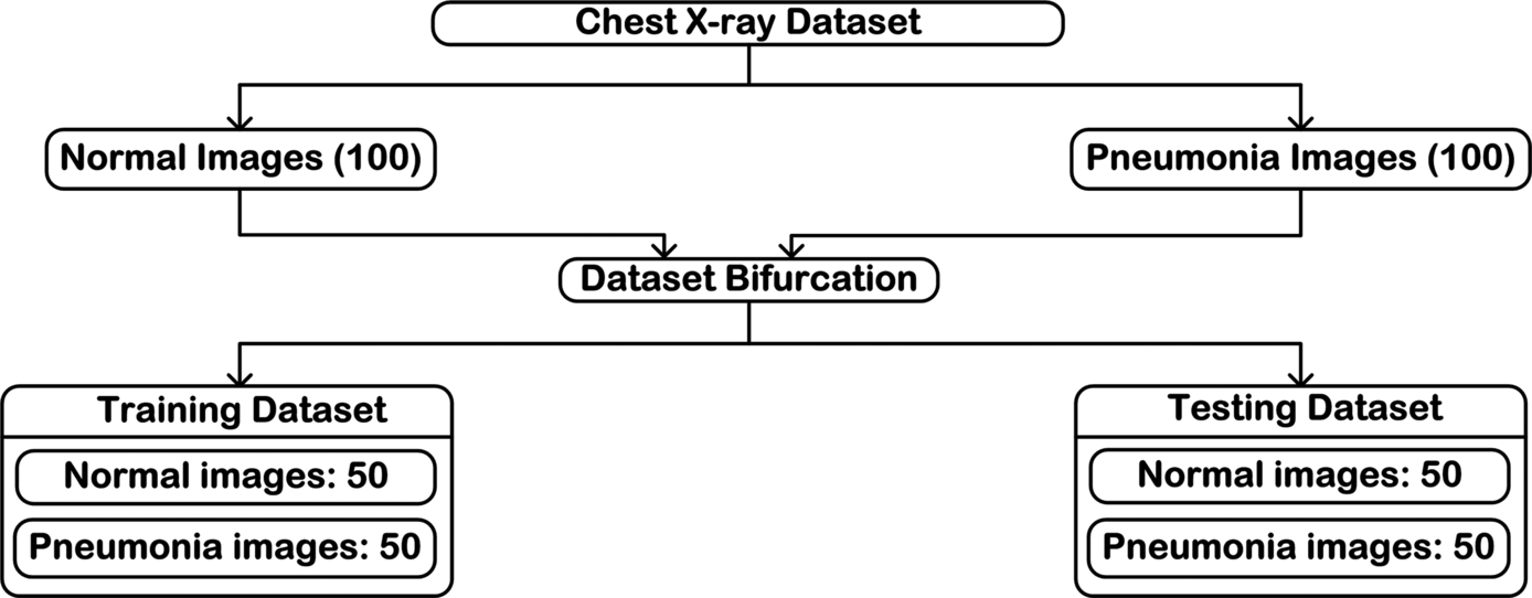
A total of 200 chest radiograph images consisting of 100 Normal chest X-ray images and 100 Pneumonia chest X-ray images have been considered for analysis. The resolution (both horizontal and vertical) of each chest radiograph image in the present dataset used is of 96 dpi. The 200 selected images are bifurcated into training dataset and testing dataset. From here the training dataset is augmented to meet the basic demand of deep learning (large amount of data), and the testing data is kept aside to perform final testing of the designed CAC systems.
3.11: Dataset generation
The experiments have been conducted using a comprehensive image dataset of 200 chest radiographs with cases of the image classes: Normal and Pneumonia. The image database is comprised of 100 Normal chest radiographs and 100 Pneumonia chest radiographs. The present work focuses on the design of CAC systems for the efficient diagnosis of Pneumonia disease using chest radiographs, which includes the foremost step of dataset generation.
The dataset generation is simply divided into three modules namely:
- (a) Preprocessing module: This deals with the image resizing and cropping to the required size of the experiment.
- (b) Dataset bifurcation: This aims at dividing the dataset generated into training, validation, and testing sets.
- (c) Augmentation module: This deals with increasing the size of the dataset by applying geometrical transformations (rotation, translation, and flipping).
The steps followed for the dataset generation for the task of classification and deep feature extraction of chest radiograph images is shown in Fig. 3.42.

3.11.1: Preprocessing module: Image resizing
The deep learning-based networks that are Pre-trained have a fixed input size of the images. Hence in order to train the network on the desired data, the images are resized to match the fixed input size of these Pre-trained networks. Hence before training the networks on the desired dataset, these images are resized to the appropriate sizes matching the predefined desired acceptable input sizes of the networks.
For the characterization of chest radiograph images, it is significant to know that the shape (morphology) of the lung in the chest radiograph image is considered significant in the process of diagnosis of Pneumonia. Therefore resizing the image directly with an aim to get the acceptable network input image size and thereby not focusing on preserving the aspect ratio of the image sometimes results in distortion of the shape of the lung when compared to the original chest radiographic image. The schematic representation of the preprocessing module is shown in Fig. 3.43.

In the present work to preserve the shape of the lung in the resized chest radiograph images, the original images have been resized by preserving their aspect ratio keeping in mind the aim of getting the acceptable network input image size of the network architecture. The process for the image resizing followed in the present work is demonstrated in Fig. 3.44.

The first step of resizing the chest radiographs to the desired size includes the generation of images that are square in shape while maintaining the aspect ratio. This is carried out by scaling the minor side of the original radiographic image to the size of the desired side.
Here the minor side refers to the side that is shorter in the original image. Henceforth, from the resulting intermediate image with an aim to get the final desired image, a random crop of the desired size is taken. This random crop marks the concluding step of getting the final desired sized image. Let original chest radiographic image have size LA × BA, with LA > BA, then according to the first step of resizing, the minor side, which is the breadth of the original radiographic image (BA), is scaled to the desired breadth size BD. This results in the formation of an intermediate chest radiographic image having the size LA × BD (where only the minor edge is similar to the desired side). Then, according to the steps of image resizing, from this intermediate chest radiographic image the length LA needs to be cropped to the desired length of LD. This final cropping of the length generates the desired resized square image having the image size LD × BD.
The following code snippets show how the image resizing is performed using MATLABR2020a to carry out the present work. Code Snippet 3.1 gives the syntax of how to access the chest radiographs from the folder in your computer.
Once the chest radiographs are read successfully, the next step is to determine the color channels of the images. Code Snippet 3.2 gives the syntax of how to determine the individual red, green, and blue color channels of the images. After determining the color channels, the next step is to obtain the actual size of the input chest radiograph. The predefined size() function of MATLAB is used here.
After obtaining the actual size of the inputimage, the next step is to calculate the aspect ratio so that the image can be preserved during resizing. Code Snippet 3.3 gives the syntax of how to calculate the aspect ratio of the original image.
Here after calculating the aspect ratio and initializing the desired size of the image, the process of resizing begins. Code Snippet 3.4 gives the syntax of performing image resizing. After resizing the resultant image is the intermediate image as discussed before. To this image random cropping is applied to obtain the final resized image.
To obtain the final resized image, the last step of random cropping is given in Code Snippet 3.5.
3.11.2: Dataset bifurcation
The schematic representation of the bifurcation of resized chest radiographs dataset into training, validation, and testing datasets before the data augmentation is shown in Fig. 3.45.

The dataset used in the present work has been primarily divided into training, validation, and testing sets. From whole dataset, half of the data (i.e., 50%) is randomly selected to form the testing dataset. The remaining half forms the training dataset, which is further divided into a ratio of 90% training data and 10% validation data. To these final training and validation datasets multiple data augmentation techniques (as further discussed in this chapter) were applied as an attempt to increase the number of representative cases in a balanced manner so that the number of augmented Normal chest radiograph images are equivalent to the number of Pneumonia chest radiograph images. The schematic representation of the dataset division is shown in Fig. 3.46.

Another important factor that was taken care of while allocating the data and forming two sets of training and validation was that for an individual image, the original as well as all the versions formed after augmentation of that chest radiograph were the part of the same set, either training or validation.
3.11.3: Augmentation module: Dataset augmentation
The deep learning-based CAC systems are state-of-the-art and require a huge amount of labeled training data to gain high accuracy and build efficient systems. Data augmentation deals with increasing the diversity of the data, thereby enabling the researchers to train their models more efficiently with diversified data without actually collecting it. The performance of deep learning techniques has high dependency on the amount of data available. Therefore, to compensate the lack of data availability, various data augmentation techniques are utilized with an aim to drastically increase the number of images available [60–63]. Hence, it can be simply understood as an essential technique that virtually increases the sample size by utilizing the actual data available.
3.11.3.1: Motivation for data augmentation
Data augmentation is pivotal in cases where the actual data is very limited and procuring new samples of the ground truth data is an expensive and time-intensive task. These problems are often faced while working with data related to medical images where there is scarcity of data. In such cases data augmentation is a highly beneficial technique for increasing the sample size. Some of the major reasons that have led to the immense use of data augmentation techniques are given as follows:
- • Data unavailability: One of the major motivations of using data augmentation is the unavailability of data for training deep learning models, specifically medical images. Acquiring access to patient medical records is a time-draining, tedious task that results in very few datasets being available for medical image analysis. The generation of medical datasets requires agreement on the patients’ behalf, and patient data security and patient privacy are other concerns. Data augmentation helps researchers increase the quantity of available data while maintaining the quality similar to the original images and fulfilling the requirements of training the deep learning models.
- • Class imbalance: Another one of the benefits of data augmentation is to overcome class imbalance. One can apply various data augmentation techniques to any particular class of the dataset or to the entire dataset to balance the numbers equally and perform the required task of prediction or classification on the augmented dataset.
- • Variation in data: Data augmentation not only increases the number of samples but also brings about variation in data as it increases the sample of unseen data for the deep learning model. Variation in data helps toward generalizability of the model, which is highly aspired while training the deep learning model. Some of the techniques, such as feature space augmentation, GAN networks, and neural style transfer are popular for introducing maximum variation in existing dataset.
- • Ease the work of researchers and cost-effectiveness: Data augmentation increases the sample space virtually without the labor intensive work of manually collecting the data, which is cost-effective in terms of both money and time. In the case of medical imaging, substantial domain specific expertise is required to generate well-labeled and well-annotated datasets. Here augmentation saves the need for medical experts and plays an important role in generating well-labeled datasets.
- • Implicit regularization: The various deep learning-based models in the absence of appropriate regularization often result in overfitting of the training data. Hence with an aim to significantly reduce the problem along with simultaneously increasing the classification and prediction performance of the model on the test data (unseen data), multiple data augmentation techniques are applied. The data augmentation aids in increasing the generalizability of the deep learning model.
3.11.3.2: Why augment only the training dataset?
Augmentation is applied with an aim to increase the sample size of the available dataset. The large size of the dataset is desirable to facilitate generalized training of the designed CAC system or network to achieve robust training and reduce overfitting. Hence larger sample space is required for the purpose of training the system. Whereas the purpose of a test dataset is to determine the error in the system designed that it will face in real time. Hence test data should be kept as close to real cases as possible. There remains no motivation for increasing the sample size of the test dataset as the required optimal model parameters are already available and it would just be a waste of time and resources to perform augmentation without any motivation. Often augmentation of test sets result in change of class labels and may adulterate the prediction accuracy of the trained model. These reasons support that data augmentation is beneficial in most cases when being applied only to the training datasets.
3.11.3.3: How to choose data augmentation technique for medical images
The data augmentation techniques for medical images are chosen in such a way that the class labels and the features that are diagnostically important to a specific tissue are preserved. The augmentation approaches used for natural images may not work for medical images as a lot of medical images are a top-down solved problem, not bottom-up like natural images. For different tissues there are different features that are considered clinically significant and pivotal for diagnosis. The features that are diagnostically important are texture, shape, and color features. For brain tumor and examination of liver ultrasounds, the texture features are primarily taken into consideration by the radiologists [64–68]. Whereas for chest radiographs, breast ultrasound, and fundus image analysis, the texture and shape features are diagnostically essential [30, 31, 68–74]. For histopathology images, the color and texture information are considered the key features for clinical diagnosis [20, 21]. For blood smear images, the features that are of prime concern are texture, color, and shape; all the three features are significant in diagnosis [75–77]. The key features of medical images have already been discussed in Chapter 1.
3.11.3.4: Types of data augmentation techniques
The recent growth in the field of radiological medical imaging techniques and digitization of records have made medical image analysis a hub for application of deep learning-based models. However, the need for large amounts of data to train these deep learning models is a challenge. The design of medical image datasets is a complex task involving the need for medical experts, time for annotation of the datasets, and some concerns such as consensus of the patient, patient privacy, and data security. Here data augmentation plays an instrumental role in generating new well-labeled data based on the existing data to increase the sample space for training the models and achieve generalizability while maintaining high performance.
For data augmentation purposes, a number of techniques have been utilized that include affine or geometrical transformation, random cropping, intensity-based methods, adding noise, color jittering, and so forth [5–9, 19]. The data augmentation techniques can broadly be of two types:
- (a) White-box techniques: These techniques are generic in nature and focus on transforming the original images in such a way that their labels are preserved. They include the following methods:
- • Geometrical transformations: This is the utmost generic type of augmentation performed and is most popular, often known as affine transformations. It includes cropping, scaling, shearing, rotation, translation, random crop, and so forth.
- • Photometric transformation: This is another one of the generic augmentation methods but is to be used carefully as it is applicable to color images and may be detrimental to the features of medical images. It includes transformations such as color jittering, fancy PCA, sharpening, and blurring of images.
- • Other transformations: These include the addition of noise, image stitching, random erasing, and more.
- (b) Black-box techniques: These techniques are more complex and focus on generation of synthetic data and adding it to the original image dataset. These include techniques such as:
- • Neural style transfer: This is a data generation technique in which the style of one image is blended with the content from another image with a motive to generate the input image as content image but generated in the style of the reference style image.
- • Adversarial training: This makes the use of generative adversarial networks popularly called the GAN.
The traditional data augmentation techniques, also known as the white-box method, include the geometrical transformations, intensity (color)-based transformation, and mixing of image pixels and techniques such as random erasing. Deep learning-based augmentation techniques, also known as the black-box techniques, mainly include adversarial networks and their use for data augmentation and techniques such as meta learning and neural style transfer are all considered under this. Fig. 3.47 shows the broad classification of various data augmentation techniques where the techniques shaded in gray are used in the present work. The types of data augmentation techniques on the basis of the time at which augmentation is performed on the data samples are classified as online and offline augmentation. In online augmentation the data is augmented just before the data is to be fed to the network and is called augmentation on the go. It is usually preferred for larger datasets. The second one is the offline data augmentation in which the data is augmented beforehand. This augmentation is used for smaller datasets as they can be easily managed manually. Fig. 3.48 shows the different geometrical transformation that can be applied to the breast ultrasound image.


Similarly Fig. 3.49 shows the different geometrical transformations that can be applied to chest radiographs.

The augmentation technique to be applied on medical images exceedingly depends on the type of tissue being used as the underlying features should be preserved and should not be lost in the process of increasing the size of the dataset. For chest radiograph images the texture and shape feature are to be preserved; hence for the present work the augmentation techniques used are rotation, translation, and flipping. Fig. 3.50 shows the schematic representation of the data augmentation module used in the present work.

In the present work the same augmentation techniques are applied to both Normal and Pneumonia chest radiograph images. The original dataset is composed of 100 images (Normal: 50, Pneumonia: 50) in training and 100 images (Normal: 50, Pneumonia: 50) in testing. The training dataset of 100 images is augmented to a total of 18,100 images. Each image is at first rotated and translated resulting in 36 images and 24 images each, respectively.
These rotated and translated images are then flipped (horizontal flip and vertical flip) resulting in 108 images after rotation and flipping, similarly resulting in 72 images after translation and flipping. In total each image is augmented to result in 181 images.
Fig. 3.51 shows the data augmentation techniques applied to the dataset used in the present work.

The augmentation techniques applied in the present work are as follows:
- (a) Rotation: This is a geometrical augmentation technique that is among the most commonly and widely used techniques, especially in medical images. The image is rotated at a certain angle except in those cases where the features of the image are highly dependent on the orientation of the object. It is performed by rotating the image right or left of the axis at angle of θ. It applies the affine transformation that follows the given equation:

Where θ is varied between 5 and 180 degrees with an interval of 5 degrees each. The rotation operation results in a total of 36 images from a single original image in the present work.
Figs. 3.52 and 3.53 show rotation of original Normal chest radiograph images and original Pneumonia chest radiograph images, respectively.


Code Snippet 3.6 shows the syntax of how to access the chest radiographs from the folder in your computer. Here the chest radiographs are stored at the path “H:DataChestX-rayOriginal ImagesNormal.” This path corresponds to the Normal chest radiographs. Similarly for Pneumonia chest radiographs the path “H:DataChestX-rayOriginal ImagesPneumonia” is accessed in the present work.
Once the images have been read from the folders they are subjected to rotation using the “imrotate” predefined function by MATLAB between angles 5 and 180 degrees with an interval of 5 degrees each. Here Code Snippet 3.7 shows the rotation of the chest X-ray radiographs between angles 5 and 45 degrees with an interval of 5 each. The rotated images are then stored to the path specified in the variable “filename1,” which is “H:DataChestX-rayAugmented ImagesNormal.”
- (b) Translation: This is the shifting of pixels of the image to the right, left, up, or down the axis. This method helps in introducing positional variation in the dataset, thereby avoiding the positional bias in the data. As most of the original images are centered, a model will train for perfectly centered images. Therefore, increasing the robustness of the system translation plays a major role. When the original images are translated, the remaining space is filled with a constant value between 0 and 255 or random Gaussian noises are added. This helps in preserving the postaugmentation spatial dimensions of the image. This augmentation technique has been applied in the present work. Fig. 3.54 shows the Normal chest radiograph images translated from [1, 2, 3, …, 12] and [− 1, − 2, − 3, …, − 12]. Fig. 3.55 shows the Pneumonia chest radiograph images translated from [1, 2, 3, …, 12] and [− 1, − 2, − 3, …, − 12].

Fig. 3.54 Translation on Normal chest radiograph image. 
Fig. 3.55 Translation on Pneumonia chest radiograph image.
Code Snippet 3.6 shows the syntax of how to access the chest radiographs from the folder in your computer. Here the chest radiographs are stored at the path “H:DataChestX-rayOriginal ImagesNormal.” Once the images have been read from the folders they are subjected to translation using the “imtranslate” predefined function by MATLAB between pixel values ± 12 as shown in Code Snippet 3.8. The translated Normal chest images are then stored to the path specified in the variable “filename1,” which is “H:DataChestX-rayAugmented ImagesNormal.” Similarly the Pneumonia chest images after translation are stored at “H:DataChestX-rayAugmented ImagesPneumonia.” The values for translation are passed in pairs of two representing the x- and y-axis values [x y]. Here in Code Snippet 3.8 the value of translation f = [11 12], representing 11 pixel translation in x-direction and 12 pixel translation in y-direction. The negative values of x and y would indicate the negative of the axis w.r.t quadrant representation.
- (c) Flip: This geometrical transformation deals with flipping of the image on the horizontal axis or the vertical axis. It is often referred to as mirroring and is one of the most commonly used and easiest augmentation techniques. This augmentation technique preserves the labels of the original data while the samples generated are entirely new for the deep learning model and widely used. In some scenarios where the features are highly dependent on the position of objects in the original image, such as features of unilateral organs, this technique is not preferred. These are those organs that are present on only one side of the human body and their change of position would affect the annotations of the original data such as the spleen and pancreas. In the present work both horizontal flip and vertical flips are applied to rotated and translated images. Some other medical images on which flipping is applied are skin images.
Figs. 3.56 and 3.57 show horizontal flipping and vertical flipping of the original Normal image and original Pneumonia images, respectively.


Code Snippets 3.9 and 3.10 give the syntax of how to perform horizontal and vertical flipping on the rotated images. The images are read in the same manner as seen in Code Snippet 3.6 and then flipping is performed using the “flip” predefined function of MATLAB where the argument of the function determines the type of flip. If the argument of flip function is 1, then it is horizontal flipping, and if the argument value passed is 2, then it represents vertical flipping.
In the present work for each augmentation, the hyperparameters are varied such as the value of θ in rotation, the translation value, and the flipping axis to generate a final augmented dataset consisting of 18,100 chest radiograph images. The augmentation was performed only on the original training dataset of 100 images, and the testing data was left unaugmented.
3.12: Concluding remarks
The methodology adopted to carry out the present work on CNN-based CAC system design for chest radiographs are presented in this chapter. This chapter explains in detail the image dataset that has been used to conduct the different experiments for designing the CNN-based CAC systems in the present work as well as the methodology adopted for data augmentation, the hardware and software requirements to carry out the present work, and the hyperparameters in deep learning. The next chapter deals with the experiments conducted that focus on designing the CNN-based CAC systems for chest radiographs. The architecture of the different CNN models, the feature selection, and feature space dimensionality reduction along with different machine learning classifiers used in the present work are discussed in subsequent chapters.