
4
Fourier Transform and Signal Spectrum
Any book on DSP is not complete without a detailed discussion of the Fourier transform. There are many publications in this area, but Brigham [1] is probably the best. The fast Fourier transform (FFT) is the numerical method [2] for computing the discrete Fourier transform (DFT) of a given time series. It exploits the periodicity properties of the function ej2πk where k is an integer.
4.1 Heterodyne Spectrum Analyser
Analysing the spectrum using the superheterodyning principle is very popular due to the simple nature of its implementation. The idea is to create a relative motion between the bandpass filter (BPF) and the incoming signal spectrum:
Equation (4.1) is shown in Figure 4.1 to give a better insight. The digitised signal sk is multiplied with a frequency-swept signal xk. Note that we need to sweep using a staircase function1 not a ramp function. We have presented the results at SNR = 0 dB.
4.1.1 Spectrum Analyser
The signal xk is defined as
![]()
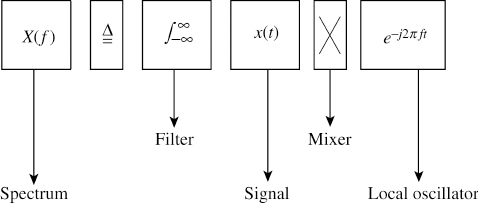
Figure 4.1 An engineer's view of (4.1)
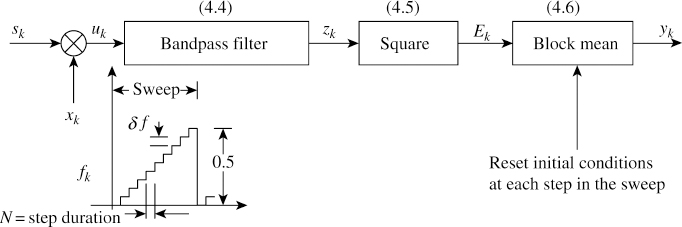
Figure 4.2 Digital spectrum analyser
The frequency fk is a staircase function totally defined by the step duration N and the step height δf = 0.5/n, where n is the number of samples of the spectrum.
A typical block diagram of this method is shown in Figure 4.2 along with the staircase function. It has three components: a BPF, a square function and a synchronised block averager. This block averager is discussed in Chapter 3 and is shown as a recursive filter. We can depict Figure 4.2 in the form of digital filters:
![]()

![]()
where the value of p lies between −2 and +2. Equation (4.6) is for obtaining the mean recursively, as described in (3.3). The initial conditions need to be reset at each step change.
4.1.1.1 Output
A spectrum analyser is implemented using r = 0.98 and p = 0 for the BPF. The staircase function is used with N = 150 and n = 200.
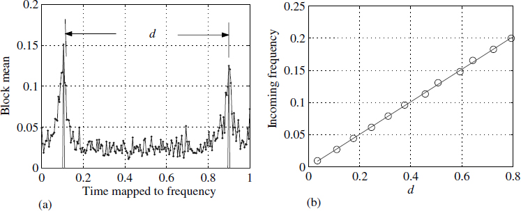
Figure 4.3 Output of a block mean filter at an SNR of 0 dB
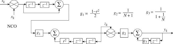
Figure 4.4 Hardware realisation of a spectrum analyser
Figure 4.4 shows a hardware realisation of the filters in (4.3) to (4.6). Figure 4.3(a) shows the output yk (4.6) for a specific value of sk. Figure 4.3(b) shows the distance between the peaks versus the input frequency of the signal sk; there is a perfect linear relation. In reality, we don't have to sweep till 0.5 Hz and it will suffice if we sweep till 0.25 Hz and find the values of yk.
4.2 Discrete Fourier Transform
The DFT relation is derived from the continuous FT of a signal. Consider a signal x(t) and its FT as
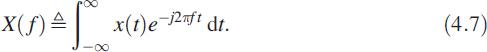
If the signal is such that x(t) = 0 for t < 0, then the FT takes the form
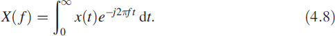
In (4.8) we replace the integral with a summation ![]() , the continuous variable t with the discrete variable n (t → n), and f with k (f → k). We get the DFT relation for sequence xn of length N:
, the continuous variable t with the discrete variable n (t → n), and f with k (f → k). We get the DFT relation for sequence xn of length N:
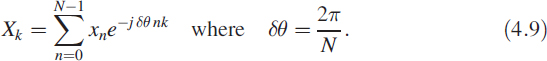
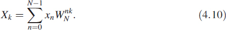
It is very convenient and mathematically tractable to use the notation WN = ej2π/N and rewrite (4.9) as
The complex quantity WN is a constant for a given value of N. Thinking of WN as cos(δθ) + j sin(δθ) will probably help you to understand it. Let us look at the transformation ![]() . This can be written as
. This can be written as ![]() , which is the same as WN/2. It may become clearer by looking at a numerical example such as
, which is the same as WN/2. It may become clearer by looking at a numerical example such as ![]() .
.
4.3 Decimating the Given Sequence
Equation (4.10) can also be written in matrix form for N points:
![]()
where S is a vector with components X1,…,XN−1.
Each row of the matrix is an FIR filter with complex coefficients (Figure 4.5), and coefficients are sampled complex cosine and sine waves. Each row can be viewed as an oscillator. The frequency of the sinewave in each row increases linearly as we move down the matrix from top to bottom. This idea was implicitly demonstrated in Chapter 3.
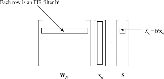
Figure 4.5 Discrete Fourier transform: understanding (4.11)
4.3.1 Sliding DFT
The transfer function of the kth row filter can also be written as an IIR filter

The pole ![]() of Hk(z) is cancelled by one of its zeros, resulting in an FIR filter. For N = 8 we get
of Hk(z) is cancelled by one of its zeros, resulting in an FIR filter. For N = 8 we get
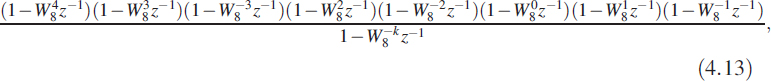
where W8 = e−jπ/4. This example shows the pole–zero cancellation. Each kth row k can also be written in the form of a difference equation:
![]()
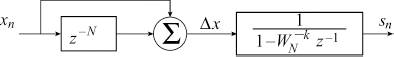
where Δx = (xn − xn−N+1) can be treated as an input to the filter.
4.4 Fast Fourier Transform
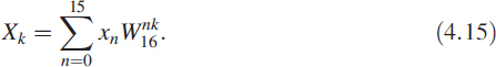
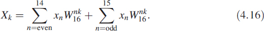
Matrix multiplication in (4.11) can be done very efficiently. Since coefficients in the matrix WN are periodic, we can arrive at a much more efficient method of computing. The given sequence can be transformed to the frequency domain by multiplying with an N × N matrix. Direct computing involves sizeable computations and is2 OO(N2) Consider a 16-point sequence of numbers for which the DFT equation is
We illustrate decimation in time and frequency with a numerical example. Note that the value of N is such that N = 2p where p is an integer.
4.4.1 Windowing Effect
A finite observation period is limited for many physical reasons and usually produces an aberration in the computed spectrum. Consider xk = cos(2πfk); mathematically, the DFT of this sequence must result in a unit sample at ±f. Numerically, let us consider f = 1/10 implying that we have chosen 10 samples/cycle, as shown in Figure 4.6(a). We have limited our observation to 32 samples. Moving from3 Figure 4.6(a) to Figure 4.6(b) can be depicted using (4.11):
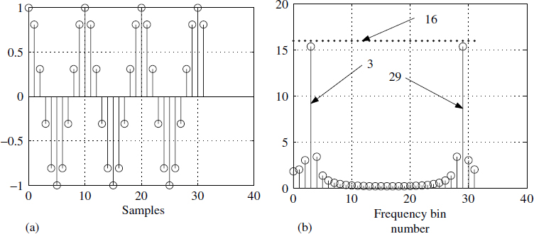
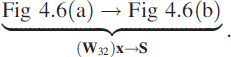
Note that Figure 4.6(b) corresponds to |S|.
Ideally, at bins 3 and 29 we should have obtained a value of 32/2 = 16 and the rest of the places should have been zero, but in reality we obtained something different, as shown in Figure 4.6(b). This spectral distortion is explained in Section 1.4. It is attributed to the fact that a rectangular window has the form ![]() and its associated leakage in the sidelobes. To mitigate the problem of limited observations, we multiply the observations point by point with another sequence w as in Figure 4.7(a). Operationally we write it as
and its associated leakage in the sidelobes. To mitigate the problem of limited observations, we multiply the observations point by point with another sequence w as in Figure 4.7(a). Operationally we write it as
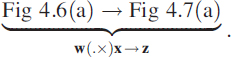
The operation (.×) denotes point-by-point multiplication of two sequences. The non-rectangular windowed spectrum is shown in Figure 4.7(b). This meets one of the criteria that the value of the spectrum be zero other than at ±f in an approximate sense.
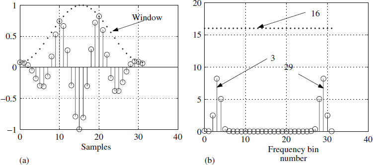
Figure 4.7 Non-rectangular windowing effect
4.4.2 Frequency Resolution
The given frequency in −0.5 to 0.5 is divided into 32 divisions, giving a resolution of δf = 1/N. The greater the observation time, the better the resolution in the spectrum. This gives us an opportunity to look at the DFT as a bank of filters separated at δf. Due to conjugate symmetry, the useful range is 0 to 15 bins.
4.4.3 Decimation in Time
We could also split the input sequence into odd and even sequences then compute the DFT. We can write (4.15) in a different way as
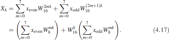
For the even case, n takes the form 2m; for the odd case, n takes the form 2m + 1. With this in mind we write (4.16) as
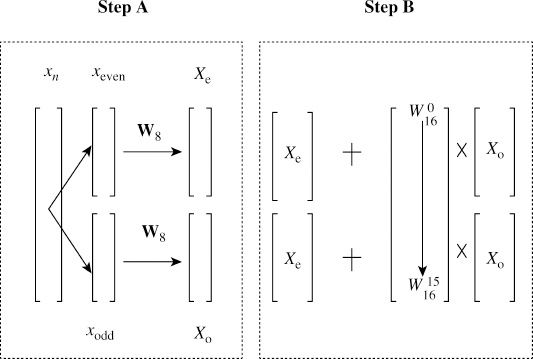
There are two steps in obtaining a 16-point DFT using an 8-point DFT. First, we divide the time sequence as odd and even or as two sets of alternating points. We compute the 8-point DFT of the two sequences, shown as step A in Figure 4.8. We replicate the odd sequence DFT to make a 16-point sequence and multiply point by point with a factor ![]() . We generate another 16-point sequence by replicating the even DFT sequence. By adding together both sequences we will get the desired 16-point DFT, shown as step B in Figure 4.8. This process is recursive, hence it leads to very efficient DFT computation.
. We generate another 16-point sequence by replicating the even DFT sequence. By adding together both sequences we will get the desired 16-point DFT, shown as step B in Figure 4.8. This process is recursive, hence it leads to very efficient DFT computation.
4.4.4 Decimation in Frequency
For decimation in frequency, we divide the sequence into two halves, premultiply with weights known as twiddle factors and compute the DFT (Figure 4.9). We rewrite (4.15) as
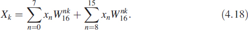
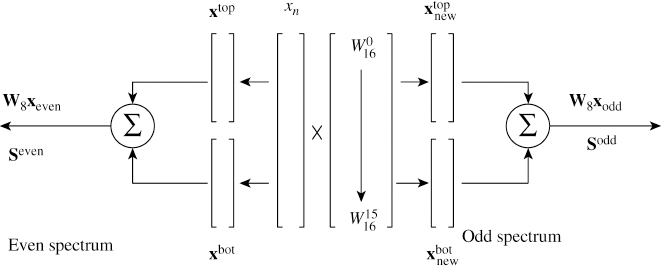
Figure 4.9 Decimation in frequency
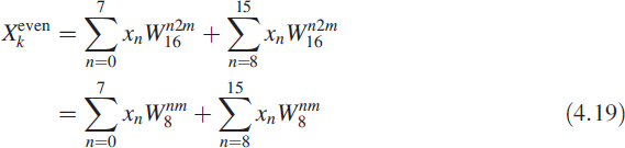
In (4.18) when k is even, we can write k = 2m for m = 0 to 7:
If we divide the sequence xn into two halves as xtop and xbot, then (4.20) has the structure
Note that even values of the spectrum are obtained by dividing the given sequence into two halves and adding them. Then we take the DFT of this new sequence, which is only half the original sequence. In (4.18) when k is odd, we can write k = 2m + 1 for m = 0 to 7:
Looking at (4.23) in detail, we have created two new sequences by doing a point-by-point multiplication with another constant sequence given as

With this notation the remaining part of the spectrum is given as
![]()
Why are we complicating things with so many variables ? The reason is that it gives us some structure. We summarise the equations as follows:
- Given the sequence we generate one more extra sequence by multiplying term by term with a complex quantity
- These two sequences are divided into two halves.
- Add corresponding halves to get two half-sequences.
- Compute the DFT of these two half-sequences.
4.4.5 Computing Effort Estimate
Consider a real sequence of length N. Computing the DFT is equivalent to multiplying an N × N complex matrix with an N-vector. Each row-by-column multiplication needs 2N multiplications and 2N additions. Assuming there is not much difference between multiplication and addition (true in the case of floating point), the total number of operations per row is 4N. For the entire matrix we need 4N2 operations. Generally it is written as OO(N2) in an engineering sense, without much detail on the minutiae of the computations.
By performing either decimation in time or frequency once, as illustrated above, we have reduced the computations from OO(N2) to OO(2(N/2)2). The computational effort has been reduced by 50%. By repeating this till we get a two-point DFT, generating a DFT becomes generating an FFT and the effort will be OO(N log2 N).
4.5 Fourier Series Coefficients
Fourier series are defined for periodic functions in time and also we assume that the integral of the function is finite. In this section we show the evaluation of Fourier series coefficients using a DFT. We take a pulse signal as an example.
4.5.1 Fourier Coefficients
Let x(t) be a continuous and periodic function of t with periodicity T, defined as
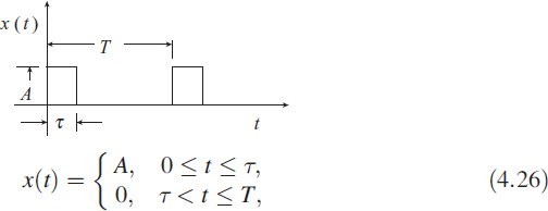

where the values of ak and bk are defined as
Let us consider a periodic function x(t) = A in the interval 0 < t < τ, otherwise x(t) = 0. For this signal, the values of ak and bk are obtained by evaluating the integrals and are given as

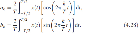
We have taken a numerical example with τ = 0.1s, T = 1.2 s and A = 1.3; we use a sampling time of 1 ms and a 512-point DFT. Figure 4.10 shows the theoretically computed coefficients superimposed with the coefficients computed using the DFT. There is a good match. Figure 4.10(a) shows the even nature of ak and Figure 4.10(b) shows the odd nature of bk. As a complex spectrum it is conjugate symmetric.
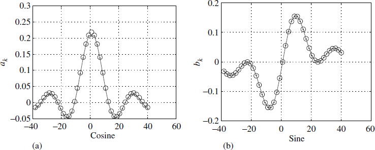
Figure 4.10 Computing Fourier coefficients using a DFT
4.6 Convolution by DFT
Convolution can be best understood in a numerical sense by looking at it as multiplication of two polynomials. We have taken this approach because polynomial multiplication is very elementary. Consider
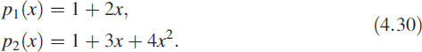
The product of the two polynomials p(x) = p1(x)p2(x) is 1 + 5x + 10x2 + 8x3 and the coefficients in p(x) are the convolution of the two sequences {1,2} and {1,3,4}. A convolution operation involves many computations. Typically, if an m-sequence is to be convolved with an n-sequence, we need to perform OO(mn) operations and the resulting sequence is of length m + n − 1. Taking the DFTs of the two sequences, multiplying them point by point and taking an inverse DFT (IDFT) will give us the desired result. FFT offers a considerable advantage in performing convolution. Exercise caution as this will result in a circular convolution.4 Let xk and yk be sequences of length m and n, respectively, then the circular convolution is defined as ![]() .
.
4.6.1 Circular Convolution
In normal convolution the sequence beyond its length is assumed to have zeros. In circular convolution the sequences are assumed to be periodic, and this produces improper results if sufficient precautions are not taken. Consider a sequence xk of length 50(m = 50) and another sequence yk of length 15(n = 15) and we perform a normal convolution to get a sequence zk = xk ⊗ yk; this is the line marked with open circles in Figure 4.11(a) and has a length of 64 (50 + 15 − 1).
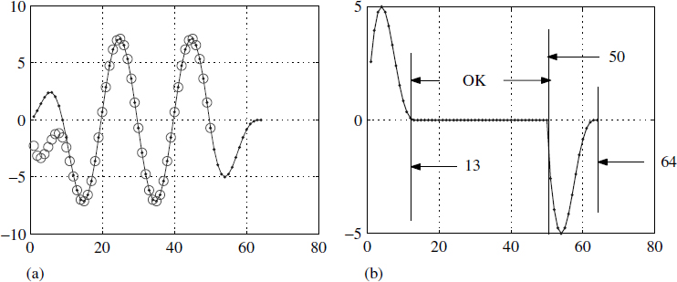
Figure 4.11 Understanding circular convolution
In Figure 4.11(a) two sequences were circularly convolved by multiplying the DFT of xk with the DFT of yk and taking the inverse DFT of the resulting sequence, leading to circular convolution ![]() . In order to take the DFTs and multiply them, we need the lengths to be the same. We have to make the lengths equal, so we have padded the sequence yk with 35 zeros. The sequence
. In order to take the DFTs and multiply them, we need the lengths to be the same. We have to make the lengths equal, so we have padded the sequence yk with 35 zeros. The sequence ![]() of length 50 is a consequence of this padding and is shown in Figure 4.11(a).
of length 50 is a consequence of this padding and is shown in Figure 4.11(a).
A comparison of the sequences zk and ![]() is shown as an error in Figure 4.11(b). It reveals that the first 12 points are erroneous and at the tail we need another 14 points of correct data. Figure 4.11(b) shows that only the length from 13 to 50 is numerically correct; the rest of the head and tail are not okay. To get over this problem we pad the sequence of length 50 with 14(= n − 1) zeros and the sequence of length 15 with 49(= m − 1) zeros, giving both sequences a length of 64 (= m + n − 1). Using these two sequences, we perform circular convolution and the result is shown in Figure 4.12 along with the regularly convolved sequence.
is shown as an error in Figure 4.11(b). It reveals that the first 12 points are erroneous and at the tail we need another 14 points of correct data. Figure 4.11(b) shows that only the length from 13 to 50 is numerically correct; the rest of the head and tail are not okay. To get over this problem we pad the sequence of length 50 with 14(= n − 1) zeros and the sequence of length 15 with 49(= m − 1) zeros, giving both sequences a length of 64 (= m + n − 1). Using these two sequences, we perform circular convolution and the result is shown in Figure 4.12 along with the regularly convolved sequence.
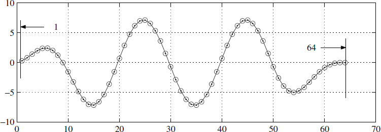
Figure 4.12 Circular convolution with right padding of zeros
4.7 DFT in Real Time
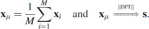
We have seen that a DFT can be computed by FFT or by recursive methods using a sliding DFT. Stability is a serious limitation of sliding DFTs. One of the most common requirements is averaging the spectrum to improve the SNR of the signal. According to Parseval's theorem, energy is conserved in the time domain or the frequency domain. And using this property, we realise that averaging in the time domain and computing the DFT is the same as computing the DFT and averaging it. Let the sequence of vectors x1, x2,…, xM have a corresponding sequence of power spectrum vectors s1,s2,…, sM. Then
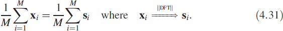
By performing a time average, we will miss the spectral update at regular intervals but we will gain on hardware complexity. What this means is that we need to wait until the ![]() computation has been completed before we can get the spectrum. To overcome this problem, inputs of two memory banks, A and B, are connected through a data switch S1 (Figure 4.13). The switch S1 is toggled between A and B when a bank is full. The output of the memory bank is also connected through a data switch S2.
computation has been completed before we can get the spectrum. To overcome this problem, inputs of two memory banks, A and B, are connected through a data switch S1 (Figure 4.13). The switch S1 is toggled between A and B when a bank is full. The output of the memory bank is also connected through a data switch S2.
When the data is being filled in A, the FFT of the data in bank B is computed by positioning S1 to A and S2 to B. On each FFT computation we perform the recursive array averaging of (4.31). Therefore by pipelining we can get a constant spectral update.
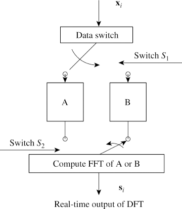
Figure 4.13 Real-time spectrum
4.7.1 Vehicle Classification
The idea of performing a time average is very important. We can use it for classifying automotive engines. Suppose we investigate a two-stroke engine and a four-stroke engine. A sequence of data zk is collected as a .wav file using a conventional media player for a sufficiently long time, say 10 s. We choose a record xi having size m = 2N, part of zk, such that when we concatenate all the xi we will obtain the original sequence zk. We average the vectors xi and compute the DFT as
Here the block mean is replaced by the recursive mean using concepts in Section 1.7. Figure 4.14(a) shows the spectrum of the averaged vector xμ for a four-stroke engine and Figure 4.14(b) shows it for a two-stroke engine. Notice the distinct difference in spectral characteristics, allowing us to obtain a parametric signature. This averaging is essential in order to obtain the features of each spectrum.
4.7.2 Instrument Classification
This is a typical problem to upgrade the single micro-phone recording to a sterio recording. Let the time series recorded using a single micro-phone in a music concert be xk. Then the problem formulation is to decompose the this time series as
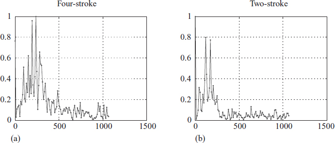
Figure 4.14 Time average spectrum
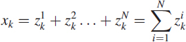
Each time series ![]() corresponds to a specific instrument say violin as if they are recorded using a seperate micro-phone. This problem is very complex and is very important in replay proving a value to the listner.
corresponds to a specific instrument say violin as if they are recorded using a seperate micro-phone. This problem is very complex and is very important in replay proving a value to the listner.
4.8 Frequency Estimation via DFT
Signals are ordinarily monochromatic in nature, but discontinuities while acquiring a signal or intentional phase variations cause its spectrum to spread. Under these conditions it is difficult to estimate the frequency by conventional methods. Here we demonstrate the use of a DFT instead of an adaptive notch filter (ANF), even though there are other ways of tackling the problem. Problems of this type occur in underwater signal processing, radar signal processing and array signal processing. Making accurate frequency estimates is a significant problem. We consider an example from radar signal processing.
4.8.1 Problem Definition
Let each signal record ri of length N be defined as
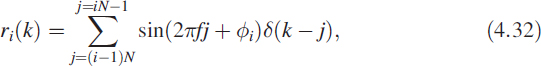
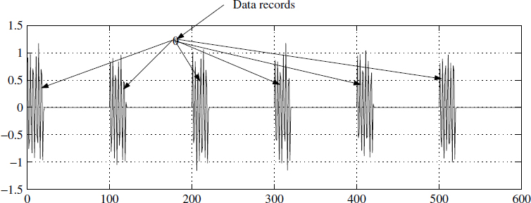
where ϕi is a uniformly distributed random phase lying between π and −π and δ(k − j) is defined as
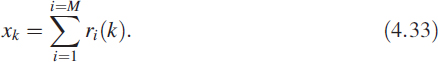
The problem is to find the frequency of the signal in the tone burst (Figure 4.15). Limitation comes from the fact that each record has a limited number of samples. So we create a new signal xk obtained by assembling M such records and given as
Unfortunately, the acquired signal suffers from rounding of noise as well as unwanted signals. So the acquired signal yk is modelled as
![]()
where γk is a white Gaussian noise (WGN) of zero mean and variance σ2. Our current problem is to accurately estimate the quantity f. There are many methods available, but in this example we have chosen a DFT approach with curve fitting in the spectral domain.
4.8.2 DFT Solution
We demonstrate how to improve resolution with a limited number of samples by combining other techniques. We consider a time series as defined in (4.34) having N = 20 and M = 6 with a WGN of variance 0.5. We get a total record length of 120 samples.
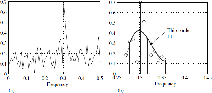
Figure 4.16 DFT of assembled records and curve fitting
For applications of this type it is best to take the DFT approach. Figure 4.16(a) shows the spectrum of the signal with a conspicuous maximum around 0.3 Hz. We have fitted a third-order polynomial around this maximum. For this polynomial we have obtained the maximum very accurately by computing the values for any desired frequency. This allows us to choose the resolution, leading to an accurate positional estimate5 of the peak, as shown in Figure 4.16(b).
Often a simple DFT computation may not suffice on its own and we need to do more manipulation to obtain better results. In the case of heterodyning spectrum analysers, similar curve fitting is performed at the output of the bandpass filter.
4.9 Parametric Spectrum in RF Systems
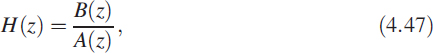
Conventional methods cannot be applied for RF systems. Impulse response is irrelevant and these systems can only be characterised using s-parameters in the S matrix. However, the notion of a transfer function exists and we can make measurements of amplitude and phase.
Frequency domain least squares (FDLS) is useful for obtaining the transfer function of the RF device. In this approach, the system under consideration is excited by fixed frequencies and output amplitude and phase are measured at steady state. Suppose we obtain the following measurements using the experimental set-up in Figure 4.17. This set-up is typical of a network analyser. The staircase is used so the system can settle down and reach steady state for measurements.
Consider the unknown device to have a model given as
![]()
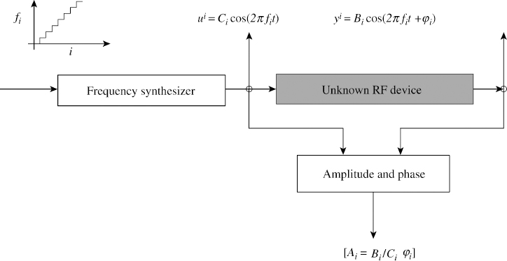
Figure 4.17 Frequency sweeping input for an unknown device
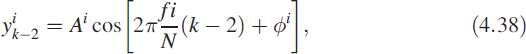
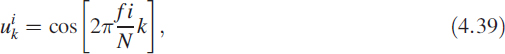
Let the input ![]() and the output measured be
and the output measured be ![]() under steady-state conditions. The term
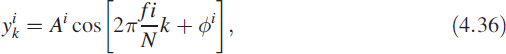
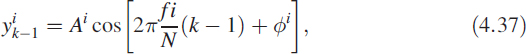
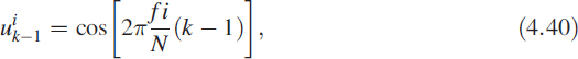
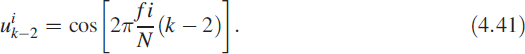
under steady-state conditions. The term ![]() is the normalised frequency. For each frequency f, measurements are made to obtain Ai and ϕi at steady state. For each measurement of Ai and ϕi at a specific frequency value of
is the normalised frequency. For each frequency f, measurements are made to obtain Ai and ϕi at steady state. For each measurement of Ai and ϕi at a specific frequency value of ![]() , yk, yk−1, yk−2, uk, uk−1, and uk−2 are computed as follows:
, yk, yk−1, yk−2, uk, uk−1, and uk−2 are computed as follows:
Now we can rewrite (4.35) using the above data as
![]()
where ![]() and pt = [a1,a2,b1,b2,b3]. For brevity, we drop the subscript k and write (4.42) as
and pt = [a1,a2,b1,b2,b3]. For brevity, we drop the subscript k and write (4.42) as
Steady-state measurement using a sweep frequency input signal offers several advantages over transient measurements such as the impulse response technique or time domain techniques [3]. Here are some of the advantages:
- Less precise instrumentation is required for steady-state measurements than for transient measurements.
- Collecting more data points improves the SNR for steady-state sweep frequency measurements, but not for transient measurements.
- Steady-state measurements offer these advantages at the expense of longer measurement time.
4.9.0.1 Simulation Results
For the purpose of simulation, we consider a system with
![]()
![]()
and we obtain output yk as
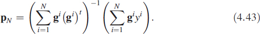
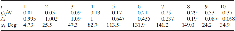
A moving-window DFT was used to monitor yk until steady-state conditions were obtained. Then (4.43) was used to obtain the solution. Results are tabulated in Table 4.1. It is also possible to estimate the order of the system using this algorithm [4].
Table 4.1 Measurements obtained using the set-up in Figure 4.17
4.9.1 Test Data Generation
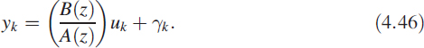
We require data to test the FDLS algorithm. This is generated synthetically. Consider a system
where B(z) and A(z) are chosen as in (4.44) and (4.45) and output yk is obtained using (4.46). The gain Ai and the phase shift ϕi of the system at a specific frequency f, as required in (4.36) to (4.42), are obtained by choosing the frequency fi then generating a sequence uk as follows:
![]()
The system is excited by uk and for k > 1000 we obtain the DFT for the sequences uk and yk as
![]()
![]()
where wk is a time-domain weighting sequence known as a Hamming window and given by
Notice that the arrays U and Y are vectors with complex elements. Let U = [U1,…,UN]. Since we know that the signal is a pure sinusoid, there will be a dominant peak in the spectrum. Hence the element of U whose magnitude is maximum is computed and the index where this maximum occurs is defined as j. Thus j = arg max |Ul| for 1 ≤ l ≤ N. Then we have
![]()
![]()
Similarly, from the complex vector Y we can obtain ![]() and
and ![]() . Now we generate the desired data as
. Now we generate the desired data as
![]()
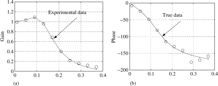
Figure 4.18 Frequency domain least-squares data
Figure 4.18 shows values of Ai and ϕi versus frequency at an SNR of 0dB for the system defined by (4.44) and (4.45). True values are superimposed on the computed values. Each true value is obtained by sampling H(z) on the unit circle at the desired frequency. Note that the values of Ai and ϕi are very accurate even when the SNR is 0 dB. This is the primary reason why the estimates are noise tolerant.
4.9.2 Estimating the Parameter Vector
Using the above data and (4.43), we get the solution as
![]()
The actual values can be obtained by looking at (4.44) and (4.45):
![]()
4.10 Summary
In this chapter we used a matrix approach to explain the principles of the FFT. We have not used butterfly diagrams. Circular convolution was explained in depth. We presented a hardware scheme for implementation in real time. We looked at a problem of estimating frequency using a DFT. We elaborated a hardware structure for real-time implementation of continuous spectrum update. We ended by covering the principles of the network analyser, an example from RF systems.
References
1. E. O. Brigham, The Fast Fourier Transform and Its Applications. Englewood Cliffs NJ: Prentice Hall, 1988.
2. J. Cooley and J. Tukey, An algorithm for the machine calculation of complex Fourier series. Mathematics of Computation, 19, 297–301, April 1965.
3. L. Ljung, System Identification Theory for the User, pp. 7–8. Englewood Cliffs NJ: Prentice Hall, 1987.
4. M. A. Soderstrand, K. V. Rangarao and G. Berchin, Enhanced FDLS algorithm for parameter-based system identification for automatic testing. In Proceedings of the 33rd IEEE Midwest Symposium on Circuits and Systems, Calgary, Canada, august 1990, pp. 96–99.
Digital Signal Processing: A Practitioner's Approach K. V. Rangarao and R. K. Mallik
© 2005 John Wiley & Sons, Ltd
1This function permits the BPF to settle down for each step change δf, as shown in Figure 4.2.
2OO is to be read as order of.
3Actually we are moving from the time domain to the frequency domain.