
Theme 2: Math and Statistics
R is a powerful statistical environment and can be used for many analytical tasks. This theme deals with various aspects of mathematical operations and statistical tests.
Topics in this Theme
- Mathematical Operations
- Summary Statistics
- Differences Tests
- Correlations and Associations
- Analysis of Variance and Linear Modeling
- Miscellaneous Methods
Commands in this Theme:
Mathematical Operations
You can think of R as a powerful calculator; many commands relate to various aspects of math.
What’s In This Topic:
- Mathematical operators
- Logarithms
- Cumulative operations
- Rounding values
- Logical operators
- Comparisons (relational operators)
- Trigonometric commands
- The constant, Pi
- Hyperbolic commands
Math
R uses a wide range of commands that carry out many different mathematical operations.
Command Name
absThis command returns the absolute magnitude of a numeric value (that is, ignores the sign). If it is used on a logical object the command produces 1 or 0 for TRUE or FALSE, respectively.
Common Usage
abs(x)Related Commands
Command Parameters
| x | An R object, usually a vector. The object can be numeric or logical. |
Examples
  ## Make a numeric vector containing positive and negative values
> xx = seq(from = -5.2, to = 5.2, by = 1)
> xx
 [1] -5.2 -4.2 -3.2 -2.2 -1.2 -0.2  0.8  1.8  2.8  3.8  4.8

  ## Get the absolute values
> abs(xx)
 [1] 5.2 4.2 3.2 2.2 1.2 0.2 0.8 1.8 2.8 3.8 4.8

  ## Make a vector of logicals
> logic = c(TRUE, TRUE, FALSE, TRUE, FALSE)
> logic
[1]  TRUE  TRUE FALSE  TRUE FALSE

  ## Get a numeric representation of the logicals
> abs(logic)
[1] 1 1 0 1 0
Command Name
Arith
+ - * ^ %% %/% /
Arithmetical operators are the general symbols used to define math operations. The +, -, *, and / are used for addition, subtraction, multiplication, and division. The ^ is used to raise a number to a power. The %% and %/% are for modulo and integer division. Arith is not a command but using help(Arith) will bring up an R help entry.
Common Usage
x + y
x – y
x * y
x / y
x ^ y
x %% y
x %/% y
Command Parameters
| x, y | Numeric or complex objects (or objects that can be coerced into one or the other). |
Examples
  ## Make a simple vector of numbers (integers)
> x = -1:12

  ## Addition
> x + 1
 [1]  0  1  2  3  4  5  6  7  8  9 10 11 12 13

  ## Compare regular and Modulo division
> x / 2
 [1] -0.5  0.0  0.5  1.0  1.5  2.0  2.5  3.0  3.5  4.0  4.5  5.0  5.5  6.0
> x %% 2
 [1] 1 0 1 0 1 0 1 0 1 0 1 0 1 0

  ## Compare regular and integer division
> x / 5
 [1] -0.2  0.0  0.2  0.4  0.6  0.8  1.0  1.2  1.4  1.6  1.8  2.0  2.2  2.4
> x %/% 5
 [1] -1  0  0  0  0  0  1  1  1  1  1  2  2  2

  ## Make a simple vector of numbers
> x = 1:6

  ## Use exponent
> 2 ^ x
[1]  2  4  8 16 32 64
Command Name
ceilingThis command rounds up a value to the nearest integer.
Common Usage
ceiling(x)Related Commands
Command Parameters
| x | A vector of numeric values. |
Examples
  ## Make some simple numeric values
> xx = seq(from = -2, to = 2, by = 0.3)
> xx
 [1] -2.0 -1.7 -1.4 -1.1 -0.8 -0.5 -0.2  0.1  0.4  0.7  1.0  1.3  1.6  1.9

  ## Round up to the nearest integer
> ceiling(xx)
 [1] -2 -1 -1 -1  0  0  0  1  1  1  1  2  2  2
Command Name
cummax
cummin
cumprod
cumsum
Cumulative values. For a vector of values these commands produce cumulative maximum, minimum, product, and sum, respectively.
Common Usage
cummax(x)
cummin(x)
cumprod(x)
cumsum(x)
Related Commands
Command Parameters
| x | A numeric object. For cumprod or cumsum this can contain complex numbers. |
Examples
  ## Cumulative product
> cumprod(1:9)
[1]      1      2      6     24    120    720   5040  40320 362880

  ## Make a vector of numbers
> xx = c(3:1, 2:0, 4:2)
> xx
[1] 3 2 1 2 1 0 4 3 2

  ## Some cumulative values
> cummax(xx)
[1] 3 3 3 3 3 3 4 4 4

> cummin(x)
[1] 3 2 1 1 1 0 0 0 0

> cumprod(xx)
[1]  3  6  6 12 12  0  0  0  0

> cumsum(xx)
[1]  3  5  6  8  9  9 13 16 18
Command Name
diffReturns lagged differences for an object. The basic command works on vector or matrix objects as well as time series (ts) objects.
Common Usage
diff(x, lag = 1, differences = 1)Related Commands
Command Parameters
| x | A numeric vector, matrix, or time series object. |
| lag = 1 | The lag between items in the difference calculation. |
| differences = 1 | If this is set to a value greater than 1, the difference calculation is carried out successively the specified number of times. |
Examples
  ## Create some values
> xx = cumsum(cumsum(1:10))
> xx
 [1]   1   4  10  20  35  56  84 120 165 220

  ## Differences between successive items
> diff(xx, lag = 1)
[1]  3  6 10 15 21 28 36 45 55

  ## Increase the lag
> diff(xx, lag = 2)
[1]   9  16  25  36  49  64  81 100

  ## Second order differences
> diff(xx, lag = 1, differences = 2)
[1]  3  4  5  6  7  8  9 10

  ## Also second order differences (same as previous example)
> diff(diff(xx))
Command Name
diffinvThis command carries out discrete integration, that is, it computes the inverse function of the lagged differences. The basic command works on vector or matrix objects as well as time series (ts) objects.
Common Usage
diffinv(x, lag = 1, differences = 1, xi)Related Commands
Command Parameters
| x | A numeric vector, matrix, or time series object. |
| lag = 1 | The lag between items in the difference calculation. |
| differences = 1 | An integer value giving the order of the difference. |
| xi | The initial values for the integrals; zeros are used if missing. This can be a numeric vector, matrix, or time series. |
Examples
  xx = cumsum(cumsum(1:10)) # Original data
> xx
 [1]   1   4  10  20  35  56  84 120 165 220

> dx = diff(xx, lag = 1) # Compute lagged differences

> dx
[1]  3  6 10 15 21 28 36 45 55
> d2 = 3:10

  ## Discrete Integration
> diffinv(dx, xi = 1) # First order
 [1]   1   4  10  20  35  56  84 120 165 220

> diffinv(d2, lag = 1, differences = 2, xi = c(1, 4)) # Second order
 [1]   1   4  10  20  35  56  84 120 165 220
Command Name
exp
expm1
Computes the exponential function. The expm1 command computes exp(x) -1.
Common Usage
exp(x)
expm1(x)
Related Commands
Command Parameters
| x | A numeric vector. |
Examples
  ## Create some values using logarithms
> xx = log(c(2, 3, 12, 21, 105))

## Produce the exponentials
> exp(xx)
[1]   2   3  12  21 105

  ## The value of e, the natural logarithm
> exp(1)
[1] 2.718282
Command Name
factorial
lfactorial
Computes the factorial, that is, x!. The lfactorial command returns the natural log of the factorial.
Common Usage
factorial(x)
lfactorial(x)
Related Commands
Command Parameters
| x | A numeric R object. |
Examples
> factorial(6)
[1] 720

> cumprod(1:6)
[1]   1   2   6  24 120 720

> lfactorial(6)
[1] 6.579251

> log(720)
[1] 6.579251
Command Name
floorThis command rounds values down to the nearest integer value.
Common Usage
floor(x)Related Commands
Command Parameters
| x | A numeric vector. |
Examples
  ## Make a vector of values
> xx = seq(from = -2, to = 2, by = 0.3)
> xx
 [1] -2.0 -1.7 -1.4 -1.1 -0.8 -0.5 -0.2  0.1  0.4  0.7  1.0  1.3  1.6  1.9

  ## Round down to nearest integer
> floor(xx)
 [1] -2 -2 -2 -2 -1 -1 -1  0  0  0  1  1  1  1
Command Name
log
log10
log2
log1p(x)
These commands compute logarithms. Natural logarithms are used by default but any base can be specified (see the following examples). The log10 and log2 commands are convenience commands for bases 10 and 2, respectively. The log1p command computes the natural log of a value + 1, that is, log(1 + x).
Common Usage
log(x, base = exp(1))
log10(x)
log2(x)
log1p(x)
Related Commands
Command Parameters
| x | A numeric or complex vector. |
| base = exp(1) | The base for the logarithm; the natural log is the default. |
Examples
  ## Logs to base 10
> log10(c(1, 10, 100, 1000))
[1] 0 1 2 3

> log(c(1, 10, 100, 1000), base = 10) # Same as previous
[1] 0 1 2 3

  ## Logs to base 2
> log2(c(2, 4, 8, 16, 32))
[1] 1 2 3 4 5

> log(c(2, 4, 8, 16, 32), base = 2) # Same as previous
[1] 1 2 3 4 5

  ## Natural logs
> log(0.2)
[1] -1.609438
> log(1.2) # Add +1 to previous value
[1] 0.1823216
> log1p(0.2) # Same as adding +1 to value
[1] 0.1823216

  ## An exotic logarithm, base Pi (~3.142)
> log(c(1, 2, 4, 8), base = pi)
[1] 0.0000000 0.6055116 1.2110231 1.8165347
Command Name
max
pmax
The max command returns the maximum value in a numerical vector or object. The pmax command returns the parallel maxima by comparing two or more objects.
Common Usage
max(..., na.rm = FALSE)
pmax(..., na.rm = FALSE)
Related Commands
Command Parameters
| ... | Vector(s) of values. These can be numeric or character (see the following examples). |
| na.rm = FALSE | By default, NA items are not omitted. |
Examples
  ## Make some numeric vectors
> xx = c(3, 3, 5, 8, 4)
> yy = c(2, 3, 6, 5, 3)
> zz = c(4, 2, 4, 7, 4)

  ## Get maxima
> max(yy)
[1] 6
> max(zz)
[1] 7

  ## Parallel maxima
> pmax(yy, zz)
[1] 4 3 6 7 4

> pmax(xx, yy, zz)
[1] 4 3 6 8 4

  ## Make character data
> pp = c("a", "f", "h", "q", "r")
> qq = c("d", "e", "x", "c", "s")

  ## Maxima
> max(pp) # Max of single vector
[1] "r"
> pmax(pp, qq) # Parallel maxima
[1] "d" "f" "x" "q" "s"
Command Name
min
pmin
The min command returns the minimum value in a vector or object (which can be numeric or character). The pmin command returns the parallel minima by comparing two objects.
Common Usage
min(..., na.rm = FALSE)
pmin(..., na.rm = FALSE)
Related Commands
Command Parameters
| ... | Vector(s) of values. These can be numeric or character (see the following examples). |
| na.rm = FALSE | By default, NA items are not omitted. |
Examples
  ## Make some numeric vectors
> yy = c(2, 3, 6, 5, 3)
> zz = c(4, 2, 4, 7, 4)

  ## Get minima
> min(yy)
[1] 2
> min(zz)
[1] 2

  ## Parallel minima
> pmin(yy, zz)
[1] 2 2 4 5 3

  ## Make character data
> pp = c("a", "f", "h", "q", "r")
> qq = c("d", "e", "x", "c", "s")

  ## Minima
> min(pp) # Min of single vector
[1] "a"
> pmin(pp, qq) # Parallel minima
1] "a" "e" "h" "c" "r"
Command Name
prodReturns the product of all the values specified.
Common Usage
prod(..., na.rm = FALSE)Related Commands
Command Parameters
| ... | Vector(s) of values. |
| na.rm = FALSE | By default, NA items are not omitted. |
Examples
  ## Make some numbers
> zz = c(4, 2, 4, 7, 4)

  ## Product
> prod(zz)
[1] 896

> 4 * 2 * 4 * 7 * 4 # Same as prod(zz)
[1] 896
Command Name
rangeGives the range for a given sample; that is, a vector containing the minimum and maximum values.
Common Usage
range(..., na.rm = FALSE)Related Commands
Command Parameters
| ... | Vector(s) of values. |
| na.rm = FALSE | By default, NA items are not omitted. |
Examples
  ## Make objects
> newvec = c(2:5, 4:5, 6:8, 9, 12, 17) # numeric vector
> vec = c(11, 15, 99, 45) # numeric vector

  ## Range
> range(newvec) # A vector containing min and max of the object
 [1] 2 17

> range(newvec, vec) # The range for the two named objects combined
 [1] 2 99
Command Name
roundRounds numeric values to a specified number of decimal places.
Common Usage
round(x, digits = 0)Related Commands
Command Parameters
| x | A numeric object, usually a vector or matrix. |
| digits = 0 | The number of decimal places to show; defaults to 0. |
Examples
  ## Make some numbers
> xx = log(2:6)
> xx
[1] 0.6931472 1.0986123 1.3862944 1.6094379 1.7917595

  ## Basic rounding
> round(xx) # Default 0 digits
[1] 1 1 1 2 2

> round(xx, digits = 2) # Two digits
[1] 0.69 1.10 1.39 1.61 1.79

  ## Effects of 0.5 (rounds to even digit)
  ## Make some values
> vv = 0.5 + -4:4
> vv
[1] -3.5 -2.5 -1.5 -0.5  0.5  1.5  2.5  3.5  4.5

> round(vv) # Use 0 digits
[1] -4 -2 -2  0  0  2  2  4  4

 ## Add a tiny amount to each value for rounding
> round(vv + sign(vv) * 1e-10)
[1] -4 -3 -2 -1  1  2  3  4  5
Command Name
signThis command returns the sign of elements in a vector. If negative an item is assigned a value of –1; if positive, +1; and if zero, 0.
Common Usage
sign(x)Related Commands
Command Parameters
| x | An R object, usually a vector or matrix object. |
Examples
  ## Make some values
> xx = -3:3
> xx
[1] -3 -2 -1  0  1  2  3

  ## Return the signs of the values
> sign(xx)
[1] -1 -1 -1  0  1  1  1

  ## Make a matrix
> mat = matrix(c(2, 3, -2, -6, -2, 5, 0, 7, -5), ncol = 3)
> mat
     [,1] [,2] [,3]
[1,]    2   -6    0
[2,]    3   -2    7
[3,]   -2    5   -5

  ## Return absolute values
> abs(mat)
     [,1] [,2] [,3]
[1,]    2    6    0
[2,]    3    2    7
[3,]    2    5    5
Command Name
signifThis command returns a value rounded to the specified number of significant figures.
Common Usage
signif(x, digits = 6)Related Commands
Command Parameters
| x | A numeric object, usually a vector or matrix (can be complex numbers). |
| digits = 6 | The number of digits to use; defaults to 6. |
Examples
  ## Make some numbers
> xx = log(2:6)
> xx
[1] 0.6931472 1.0986123 1.3862944 1.6094379 1.7917595

  ## Show 3 digits
> signif(xx, digits = 3)
[1] 0.693 1.100 1.390 1.610 1.790

  ## Make some large numbers
> yy = 2^(12:20)
> yy
[1]    4096    8192   16384   32768   65536  131072  262144  524288 1048576

  ## Show 3 digits
> signif(yy, digits = 3)
[1]    4100    8190   16400   32800   65500  131000  262000  524000 1050000

  ## Display 3 digits
> signif(c(3.1683564e+1, 235467, 0.1134597898), digits = 3)
[1] 3.17e+01 2.35e+05 1.13e-01

  ## Small values displayed to 3 digits
> signif(0.0000000000012345678, digits=3)
[1] 1.23e-12

> signif(1.2345678e-12, digits=3)
[1] 1.23e-12
Command Name
sqrtDetermines the square root of a numerical object, that is, sqrt(2) is the same as 2^0.5.
Common Usage
sqrt(x)Related Commands
Command Parameters
| x | A numerical R object, usually a vector or matrix object (can contain complex numbers). |
Examples
> sqrt(1:9)
[1] 1.000000 1.414214 1.732051 2.000000 2.236068 2.449490 2.645751 2.828427
[9] 3.000000
Command Name
sumThis command returns the sum of all the items specified.
Common Usage
sum(..., na.rm = FALSE)Related Commands
Command Parameters
| ... | Numeric R object(s). Usually a vector or matrix, but complex and logical objects can also be specified. |
| na.rm = FALSE | If na.rm = TRUE, then NA items are omitted. |
Examples
  ## Make some values
> xx = 1:9
> xx
[1] 1 2 3 4 5 6 7 8 9

  ## Determine the sum
> sum(xx)
[1] 45

  ## Make more values
> yy = c(2, 3, 6, 5, 3)
> yy
[1] 2 3 6 5 3

  ## Determine sums
> sum(yy) ## Just sum of yy
[1] 19

> sum(xx, yy) # Sum of xx and yy together
[1] 64

  ## Make a logical vector
> logic = c(TRUE, TRUE, FALSE, TRUE, FALSE)

  ## Sum the logical (total of TRUE items)
> sum(logic)
[1] 3
Command Name
truncCreates integer values by truncating items at the decimal point.
Common Usage
trunc(x)Related Commands
Command Parameters
| x | A numeric vector. |
Examples
  ## Make some numbers
> xx = 0.5 + -2:4
> xx
[1] -1.5 -0.5  0.5  1.5  2.5  3.5  4.5

  ## Truncate to integer
> trunc(xx)
[1] -1  0  0  1  2  3  4

  ## Round values to 0 decimal
> round(xx)
[1] -2  0  0  2  2  4  4
Logic
Many R commands produce logical values (that is, TRUE or FALSE). Logical operators and comparisons (relational operators) are used in many commands to make decisions and to produce results that match logical criteria.
Command Name
allThis command returns a logical value TRUE if all the values specified are TRUE.
Common Usage
all(..., na, rm = FALSE)Related Commands
Command Parameters
| ... | Logical vectors or an expression that returns a logical result. |
| na.rm = FALSE | If na.rm = TRUE, then NA items are omitted. |
Examples
  ## A vector of values
> yy = c(2, 3, 6, 5, 3)

  ## Test all items in vector to a condition
> all(yy < 5)
[1] FALSE

> all(yy >= 2)
[1] TRUE
Command Name
all.equalTests to see if two objects are (nearly) equal. The result is a logical TRUE or FALSE.
Common Usage
all.equal(target, current, tolerance = .Machine$double.eps ^ 0.5)Related Commands
Command Parameters
| target | An R object to be compared to the current. |
| current | An R object to be compared to the target. |
| tolerance | A numerical value to be considered as different. The value must be ≥ 0. If the tolerance is set to 0, the actual difference is shown. The default tolerance equates to around 1.49e-08. |
Examples
  ## Some simple values
> x1 = 0.5 - 0.3
> x2 = 0.3 - 0.1

  ## Are objects the same?
> x1 == x2
[1] FALSE

  ## Set tolerance to 0 to show actual difference
> all.equal(x1, x2, tolerance = 0)
[1] "Mean relative difference: 1.387779e-16"

  ## Use default tolerance
> all.equal(x1, x2)
[1] TRUE

  ## Wrap command in isTRUE() for logical test
> isTRUE(all.equal(x1, x2))
[1] TRUE

> isTRUE(all.equal(x1, x2, tolerance = 0))
[1] FALSE

  ## Make some character vectors
> pp = c("a", "f", "h", "q", "r")
> qq = c("d", "e", "x", "c", "s")

  ## Test for equality
> all.equal(pp, qq)
[1] "5 string mismatches"
Command Name
anyThis command returns a logical value TRUE if any of the values specified are TRUE.
Common Usage
any(..., na.rm = FALSE)Related Commands
Command Parameters
| ... | Logical vectors or an expression that returns a logical result. |
| na.rm = FALSE | If na.rm = TRUE, then NA items are omitted. |
Examples
  ## Make some values to test
> yy = c(2, 3, 6, 5, 3)

  ## Test if any element matches a condition
> any(yy == 3)
[1] TRUE

> any(yy > 6)
[1] FALSE
Command Name
Comparison
< > <= >= == !=
These symbols allow the representation of comparisons; they are relational operators. The < and > symbols represent “less than” and “greater than,” respectively. The <= and >= symbols represent “less than or equal to” and “greater than or equal to,” respectively. The == and != symbols represent “equal to” and “not equal to,” respectively. The results are a logical, either TRUE or FALSE. Comparison is not a command but using help(Comparison) will bring up an R help entry.
Common Usage
x < y
x > y
x <= y
x >= y
x == y
x != y
Related Commands
Command Parameters
| x, y | R objects or values. |
Examples
  ## Make some numbers
> zz = c(4, 2, 4, 7, 4)
> zz
[1] 4 2 4 7 4

  ## Logic tests
> zz == 4 # Shows which are equal to 4
[1]  TRUE FALSE  TRUE FALSE  TRUE

> zz <= 4 # Shows which are equal or less than 4
[1]  TRUE  TRUE  TRUE FALSE  TRUE

> zz != 4 # Shows which are not equal to 4
[1] FALSE  TRUE FALSE  TRUE FALSE

  ## Use braces to return values
> zz[zz != 4] # Shows items that are not equal to 4
[1] 2 7

  ## Beware of rounding errors
  ## Create some values
> xx = seq(from = -1, to = , by = 0.3)
> xx
[1] -1.0 -0.7 -0.4 -0.1  0.2  0.5  0.8

> xx == 0.2 # Nothing is TRUE because of precision
[1] FALSE FALSE FALSE FALSE FALSE FALSE FALSE

> round(xx, digits = 1) == 0.2 # Use rounding get TRUE result
[1] FALSE FALSE FALSE FALSE  TRUE FALSE FALSE
Command Name
isTRUEThis command tests to see if an object or result is TRUE. It is useful as a wrapper for other commands where a single non-logical result could occur, for example, the all.equal command.
Common Usage
isTRUE(x)Related Commands
Command Parameters
| x | An R object. |
Examples
  ## Simple values to compare
> x1 = 0.5 - 0.3
> x2 = 0.3 - 0.1

  ## Comparisons
> x1 == x2 # Gives FALSE because of precision
[1] FALSE

> isTRUE(all.equal(x1, x2)) # Gives a TRUE result
[1] TRUE

> all.equal(x1, x2, tolerance = 0) # Gives a non-logical result
[1] "Mean relative difference: 1.387779e-16"

> isTRUE(all.equal(x1, x2, tolerance = 0)) # Gives a logical result
[1] FALSE
Command Name
Logic
! & && | || xor
These symbols are used to define logical operators and so define comparisons. The ! symbol indicates logical NOT. The & and && symbols indicate logical AND. The | and || symbols indicate logical OR. The xor symbol indicates exclusive OR. The single symbols & and | perform element-wise comparisons. The longer && and || evaluate left to right, examining only the first element of each vector. Logic is not a command but typing help(Logic) will bring up a help entry.
Common Usage
! x
x & y
x && y
x | y
x || y
xor(x, y)
Related Commands
Command Parameters
| x, y | R objects for comparison. |
Examples
  ## Make vectors to compare
> yy = c(2, 3, 6, 5, 3)
> zz = c(4, 2, 4, 7, 4)
> yy ; zz
[1] 2 3 6 5 3
[1] 4 2 4 7 4

  ## Comparisons
> yy > 2 & zz > 4 # One condition AND another
[1] FALSE FALSE FALSE  TRUE FALSE

> yy > 3 | zz > 4 One condition OR another
[1] FALSE FALSE  TRUE  TRUE FALSE

> ! yy > 3 Test for items NOT greater than 3
[1]  TRUE  TRUE FALSE FALSE  TRUE

  ## Contrast single and double operators
> yy == 2 | zz > 3 # Multiple result
[1]  TRUE FALSE  TRUE  TRUE  TRUE

> yy == 2 || zz > 3 # Single result (1st element from previous)
[1] TRUE

> yy > 2 | zz > 4 # Multiple result
[1] FALSE  TRUE  TRUE  TRUE  TRUE

> yy > 2 || zz > 4 # Single result (1st element from previous)
[1] FALSE
Complex Numbers
Complex numbers can be dealt with by many commands. However, several commands are designed to create, test, and extract elements of complex numbers. In addition, complex numbers hold a class attribute "complex".
Command Name
ArgReturns the argument of an imaginary number.
Common Usage
Arg(z)Related Commands
Command Parameters
| z | A complex number or an R object that holds a class attribute "complex". |
Examples
  ## Make some complex numbers
> z0 = complex(real = 1:8, imaginary = 8:1)
> z1 = complex(real = 4, imaginary = 3)
> z2 = complex(real = 4, imaginary = 3, argument = 2)
> z3 = complex(real = 4, imaginary = 3, modulus = 4, argument = 2)

> z0 ; z1 ; z2; z3
[1] 1+8i 2+7i 3+6i 4+5i 5+4i 6+3i 7+2i 8+1i
[1] 4+3i
[1] -0.4161468+0.9092974i
[1] -1.664587+3.63719i

  ## Display the arguments
> Arg(z0)
[1] 1.4464413 1.2924967 1.1071487 0.8960554 0.6747409 0.4636476 0.2782997
[8] 0.1243550

> Arg(z1)
[1] 0.6435011

> Arg(z2)
[1] 2
Command Name
as.complexAttempts to coerce an object to a complex object, that is, one holding a class attribute "complex".
Common Usage
as.complex(z)Related Commands
Command Parameters
| z | An R object. |
Examples
  ## Make a character vector
> zz = c("3+2i", "4+2i")
> zz
[1] "3+2i" "4+2i"

> class(zz) # Check the class
[1] "character"

  ## Make character vector into complex
> zz = as.complex(zz)

> zz
[1] 3+2i 4+2i

> class(zz)
[1] "complex"
Command Name
complexCreates a complex number or vector of numbers. The command can also be used to create a blank vector containing a certain number of items.
Common Usage
complex(length.out = 0, real = numeric(), imaginary = numeric(),
        modulus = 1, argument = 0)
Related Commands
Command Parameters
| length.out = 0 | The number of elements to create. Used to limit a sequence or to create a blank vector of complex numbers. |
| real = numeric() | The real part of the number(s). |
| imaginary = numeric() | The imaginary part of the number(s). |
| modulus = 1 | The modulus of the complex number(s). |
| argument = 0 | The argument of the complex number(s). |
Examples
  ## A blank complex vector
> zz = complex(length.out = 3)
> zz
[1] 0+0i 0+0i 0+0i

  ## Some complex numbers as vectors
> z0 = complex(real = 1:8, imaginary = 8:1)
> z1 = complex(real = 4, imaginary = 3)
> z2 = complex(real = 4, imaginary = 3, argument = 2)
> z3 = complex(real = 4, imaginary = 3, modulus = 4, argument = 2)

> z0 ; z1 ; z2; z3
[1] 1+8i 2+7i 3+6i 4+5i 5+4i 6+3i 7+2i 8+1i
[1] 4+3i
[1] -0.4161468+0.9092974i
[1] -1.664587+3.63719i
Command Name
ConjDisplays the complex conjugate for a complex number.
Common Usage
Conj(z)Related Commands
Command Parameters
| z | A complex number or an R object that holds a class attribute "complex". |
Examples
  ## Make some complex numbers
> z0 = complex(real = 1:8, imaginary = 8:1)
> z1 = complex(real = 4, imaginary = 3)
> z2 = complex(real = 4, imaginary = 3, argument = 2)
> z3 = complex(real = 4, imaginary = 3, modulus = 4, argument = 2)

> z0 ; z1 ; z2; z3
[1] 1+8i 2+7i 3+6i 4+5i 5+4i 6+3i 7+2i 8+1i
[1] 4+3i
[1] -0.4161468+0.9092974i
[1] -1.664587+3.63719i

  ## The complex conjugates
> Conj(z0)
[1] 1-8i 2-7i 3-6i 4-5i 5-4i 6-3i 7-2i 8-1i

> Conj(z1)
[1] 4-3i

> Conj(z2)
[1] -0.4161468-0.9092974i

> Conj(z3)
[1] -1.664587-3.63719i
Command Name
ImShows the imaginary part of a complex number.
Common Usage
Im(z)Related Commands
Command Parameters
| z | A complex number or an R object that holds a class attribute "complex". |
Examples
  ## Make some complex numbers
> z0 = complex(real = 1:8, imaginary = 8:1)
> z1 = complex(real = 4, imaginary = 3)
> z2 = complex(real = 4, imaginary = 3, argument = 2)
> z3 = complex(real = 4, imaginary = 3, modulus = 4, argument = 2)

> z0 ; z1 ; z2; z3
[1] 1+8i 2+7i 3+6i 4+5i 5+4i 6+3i 7+2i 8+1i
[1] 4+3i
[1] -0.4161468+0.9092974i
[1] -1.664587+3.63719i

  ## Show the imaginary part of the numbers
> Im(z0)
[1] 8 7 6 5 4 3 2 1

> Im(z1)
[1] 3

> Im(z2)
[1] 0.9092974

> Im(z3)
[1] 3.63719
Command Name
is.complexTests to see if an object is a complex object (does it have a class attribute "complex"?). The result is a logical, TRUE or FALSE.
Common Usage
is.complex(z)Related Commands
Command Parameters
| z | A complex number or an R object that holds a class attribute "complex". |
Examples
  ## Make some objects
> zz = c(3+2i, "2+4i") # Mixed so ends up as character
> z0 = c(3+2i, 4+2i) # Complex
> z1 = complex(real = 4, imaginary = 3) # Complex

> zz ; z0 ; z1
[1] "3+2i" "2+4i"
[1] 3+2i 4+2i
[1] 4+3i

  ## Test objects
> is.complex(zz)
[1] FALSE

> is.complex(z0)
[1] TRUE

> is.complex(z1)
[1] TRUE
Command Name
ModShows the modulus of a complex number.
Common Usage
Mod(z)Related Commands
Command Parameters
| z | A complex number or an R object that holds a class attribute "complex". |
Examples
  ## Make some complex numbers
> z0 = complex(real = 1:8, imaginary = 8:1)
> z1 = complex(real = 4, imaginary = 3)
> z2 = complex(real = 4, imaginary = 3, argument = 2)
> z3 = complex(real = 4, imaginary = 3, modulus = 4, argument = 2)

> z0 ; z1 ; z2; z3
[1] 1+8i 2+7i 3+6i 4+5i 5+4i 6+3i 7+2i 8+1i
[1] 4+3i
[1] -0.4161468+0.9092974i
[1] -1.664587+3.63719i

  ## The modulus
> Mod(z0)
[1] 8.062258 7.280110 6.708204 6.403124 6.403124 6.708204 7.280110 8.062258

> Mod(z1)
[1] 5

> Mod(z2)
[1] 1

> Mod(z3)
[1] 4
Command Name
ReShows the real part of complex numbers.
Common Usage
Re(z)Related Commands
Command Parameters
| z | A complex number or an R object that holds a class attribute "complex". |
Examples
  ## Make some complex numbers
> z0 = complex(real = 1:8, imaginary = 8:1)
> z1 = complex(real = 4, imaginary = 3)
> z2 = complex(real = 4, imaginary = 3, argument = 2)
> z3 = complex(real = 4, imaginary = 3, modulus = 4, argument = 2)

> z0 ; z1 ; z2; z3
[1] 1+8i 2+7i 3+6i 4+5i 5+4i 6+3i 7+2i 8+1i
[1] 4+3i
[1] -0.4161468+0.9092974i
[1] -1.664587+3.63719i

  ## Show the real parts
> Re(z0)
[1] 1 2 3 4 5 6 7 8

> Re(z1)
[1] 4

> Re(z2)
[1] -0.4161468

> Re(z3)
[1] -1.664587
Trigonometry
R contains various basic trigonometric commands and hyperbolic functions as well as pi, the constant π.
Command Name
cos
acos
cosh
acosh
These commands deal with the cosine. The commands calculate the cosine, arc-cosine, and hyperbolic equivalents. Angles are in radians (a right angle is π / 2 radians).
Common Usage
cos(x)
acos(x)
cosh(x)
acosh(x)
Related Commands
Command Parameters
| x | A numeric value to evaluate. Can be numeric vectors or complex objects. Angles are in radians. |
Examples
> cos(45) # In radians
[1] 0.525322

> cos(45 * pi/180) # Convert 45 degrees to radians
[1] 0.7071068

> acos(1/2) * 180/pi # To get result in degrees
[1] 60

> acos(sqrt(3)/2) * 180/pi # To get result in degrees
[1] 30

> cosh(0.5) # Hyperbolic function
[1] 1.127626
Command Name
piThe numeric constant π; this is approximately 3.142.
Common Usage
piRelated Commands
Command Parameters
No parameters are necessary; pi is recognized as a constant.
Examples
  ## pi is recognized as a constant
> pi
[1] 3.141593

  ## Use of pi in trigonometry
> cos(45 * pi/180) # Convert degrees to radians
[1] 0.7071068

> acos(0.5) * 180/pi # Convert radians to degrees
[1] 60

  ## 1 radian ~57 degrees
> 180/pi
[1] 57.29578
Command Name
sin
asin
sinh
asinh
These commands deal with the sine. The commands calculate the sine, arc-sine, and hyperbolic equivalents. Angles are in radians (a right angle is π / 2 radians).
Common Usage
sin(x)
asin(x)
sinh(x)
asinh(x)
Related Commands
Command Parameters
| x | A numeric value to evaluate. Can be numeric vectors or complex objects. Angles are in radians. |
Examples
> sin(45) # In radians
[1] 0.8509035

> sin(45 * pi/180) # Convert degrees to radians
[1] 0.7071068

> asin(0.5) * 180/pi # To get answer in degrees
[1] 30

> asin(sqrt(3)/2) * 180/pi # To get answer in degrees
[1] 60

> sinh(0.4) # Hyperbolic function
[1] 0.4107523
Command Name
tan
atan
atan2
tanh
atanh
These commands deal with the tangent. The commands calculate the tangent, arc-tangent, and hyperbolic equivalents. The atan2 command calculates the angle between the x-axis and the vector from the origin to (x, y). Angles are in radians (a right angle is π / 2 radians).
Common Usage
tan(x)
atan(x)
atan2(y, x)
tanh(z)
atanh(x)
Related Commands
Command Parameters
| x | A numeric value to evaluate. Can be numeric vectors or complex objects. Angles are in radians. |
| y, x | For atan2 command y, x, are coordinates. |
Examples
> tan(45) # In radians
[1] 1.619775

> tan(45 * pi/180) # Convert degrees to radians
[1] 1

> atan(0.6) * 180/pi # Get answer in degrees
[1] 30.96376

> atan(sqrt(3)) * 180/pi # Get answer in degrees
[1] 60

> tanh(0.2) # Hyperbolic function
[1] 0.1973753

  ## Find angle between coordinates and x-axis (in degrees)
> atan2(5, 5) * 180/pi
[1] 45

> atan2(10, 5) * 180/pi
[1] 63.43495

> atan2(5, 10) * 180/pi
[1] 26.56505
Hyperbolic Functions
Matrix Math
A matrix is a rectangular array with rows and columns. Many R commands are designed expressly to deal with matrix math.
Command Name
backsolve
forwardsolve
These commands solve a system of linear equations where the coefficient matrix is upper (“right”, “R”) or lower (“left”, “L”) triangular.
Common Usage
backsolve(r, x, k = ncol(r), upper.tri = TRUE, transpose = FALSE)
forwardsolve(l, x, k = ncol(l), upper.tri = FALSE, transpose = FALSE)
Related Commands
Command Parameters
| r, l | A matrix giving the coefficients for the system to be solved. Only the upper or lower triangle is used and other values are ignored. |
| x | A matrix whose columns give the right-hand sides for the equations. |
| k | The number of columns for r (or l) and rows of x to use. |
| upper.tri = | If TRUE, the upper triangle of the coefficient matrix is used; use upper.tri = FALSE to use the lower triangle. |
| transpose = FALSE | If set to TRUE, the transposed matrix is used; that is, y is solved in the equation r’ y = x. |
Examples
  ## Make a coefficient matrix
> (mx = cbind(1,1:3,c(2,0,1)))
     [,1] [,2] [,3]
[1,]    1    1    2
[2,]    1    2    0
[3,]    1    3    1

  ## The right-hand sides of the equations
> x = c(8, 4, 2)

  ## Solve
> backsolve(mx, x) # The upper triangular solution
[1] 2 2 2

> forwardsolve(mx, x) # The lower triangular solution
[1]  8 -2  0

> backsolve(mx, x, upper.tri = FALSE) # Same as previous
[1]  8 -2  0

> backsolve(mx, x, transpose = TRUE) # Transpose matrix
[1]   8  -2 -14
Command Name
cholThis command computes the Choleski factorization of a real matrix. The matrix must be symmetric, positive-definite. The result returned is the upper triangular factor of the Choleski decomposition, that is, the matrix R such that R'R = x.
Common Usage
chol(x, pivot = FALSE, LINPACK = pivot)Related Commands
Command Parameters
| x | A matrix that is real, symmetric, and positive-definite. |
| pivot = FALSE | If TRUE, pivoting is used. This can enable the decomposition of a positive semi-definite matrix to be computed. |
| LINPACK = FALSE | If set to TRUE, then for non-pivoting, the LINPACK routines are used (thus providing compatibility with older versions). |
Examples
  ## Make a matrix
> (mx = matrix(c(5,1,1,3), ncol = 2))
     [,1] [,2]
[1,]    5    1
[2,]    1    3

  ## Choleski decomposition
> (cm = chol(mx))
         [,1]      [,2]
[1,] 2.236068 0.4472136
[2,] 0.000000 1.6733201

  ## Original matrix can be reconstructed from Choleski
> crossprod(cm)
     [,1] [,2]
[1,]    5    1
[2,]    1    3

> t(cm) %*% cm
     [,1] [,2]
[1,]    5    1
[2,]    1    3
Command Name
crossprod
tcrossprod
These commands calculate the cross-products of two matrix objects. They are equivalent to t(x) %*% y (for the crossprod command) and x %*% t(y) (for the tcrossprod command).
Common Usage
crossprod(x, y = NULL)
tcrossprod(x, y = NULL)
Related Commands
Command Parameters
| x, y | Matrix objects (can be complex numbers). If y is missing it is assumed to be the same matrix as x. |
Examples
  ## Make matrix objects
> (x = cbind(1,1:3,c(2,0,1)))
     [,1] [,2] [,3]
[1,]    1    1    2
[2,]    1    2    0
[3,]    1    3    1

> (y = c(1, 3, 2))
[1] 1 3 2

> (y1 = matrix(1:3, nrow = 1))
     [,1] [,2] [,3]
[1,]    1    2    3

  ## Cross-products
> crossprod(x, y)   # Same as t(x) %*% y
     [,1]
[1,]    6
[2,]   13
[3,]    4

> crossprod(x, y1) # Gives error as y1 wrong "shape"
Error in crossprod(x, y1) : non-conformable arguments

> tcrossprod(x, y1) # Same as x %*% t(y1)
     [,1]
[1,]    9
[2,]    5
[3,]   10
Command Name
det
determinant
The determinant command calculates the modulus of the determinant (optionally as a logarithm) and the sign of the determinant. The det command calculates the determinant of a matrix (it is a wrapper for the determinant command).
Common Usage
det(x)
determinant(x, logarithm = TRUE)
Related Commands
Command Parameters
| x | A numeric matrix. |
| logarithm = TRUE | If TRUE (the default), the natural logarithm of the modulus of the determinant is calculated. |
Examples
  ## Make a matrix
> x = cbind(1,1:3,c(2,0,1))
> x
     [,1] [,2] [,3]
[1,]    1    1    2
[2,]    1    2    0
[3,]    1    3    1

  ## The determinant
> det(x)
[1] 3

  ## The longer command produces a list as a result
> determinant(x)
$modulus
[1] 1.098612
attr(,"logarithm")
[1] TRUE

$sign
[1] 1

attr(,"class")
[1] "det"

  ## Make result more readable (shows log)
> unlist(determinant(x))
 modulus     sign
1.098612 1.000000

  ## Unlist result but show non-log determinant
> unlist(determinant(x, logarithm = FALSE))
modulus    sign
      3       1
Command Name
diagMatrix diagonals. This command has several uses; it can extract or replace the diagonal of a matrix. Alternatively, the command can construct a diagonal matrix. See the following command parameters for details.
Common Usage
diag(x = 1, nrow, ncol)
diag(x) <- value
Related Commands
Command Parameters
| x | There are various options for x:
|
| nrow | Number of rows for the identity matrix (if x is not a matrix). |
| ncol | Number of columns for the identity matrix (if x is not a matrix). |
| value | A numerical value for the diagonal. This should be either a single number or a vector equal to the length of the current diagonal. |
Examples
  ## Make a matrix
> x = cbind(1,1:3,c(2,0,1))
> x
     [,1] [,2] [,3]
[1,]    1    1    2
[2,]    1    2    0
[3,]    1    3    1

  ## Get the current diagonal
> diag(x)
[1] 1 2 1

  ## Reset current diagonal
> diag(x) <- c(2, 1, 2)
> x
     [,1] [,2] [,3]
[1,]    2    1    2
[2,]    1    1    0
[3,]    1    3    2

  ## Make identity matrix
> diag(x = 3) # Simple identity matrix
     [,1] [,2] [,3]
[1,]    1    0    0
[2,]    0    1    0
[3,]    0    0    1

> diag(x = 3, nrow = 3) # Set diagonal and rows
     [,1] [,2] [,3]
[1,]    3    0    0
[2,]    0    3    0
[3,]    0    0    3

> diag(c(6, 9)) # Specify diagonal
     [,1] [,2]
[1,]    6    0
[2,]    0    9

> diag(c(7, 4), nrow = 4) # Extra rows (must be multiple of diagonal)
     [,1] [,2] [,3] [,4]
[1,]    7    0    0    0
[2,]    0    4    0    0
[3,]    0    0    7    0
[4,]    0    0    0    4
Command Name
dropThis command examines an object and if there is a dimension with only a single entry, the dimension is removed.
Common Usage
drop(x)Related Commands
Command Parameters
| x | An array or matrix object. |
Examples
  ## Simple matrix multiplication
> 1:3 %*% 2:4 # Makes a matrix with single entry
     [,1]
[1,]   20

  ## Drop redundant dimension
> drop(1:3 %*% 2:4) # Single value (vector) result
[1] 20

  ## Make an array
> my.arr = array(1:6, dim = c(3, 1, 2))
> my.arr
, , 1

     [,1]
[1,]    1
[2,]    2
[3,]    3

, , 2

     [,1]
[1,]    4
[2,]    5
[3,]    6

  ## Drop redundant dimension
> drop(my.arr)
     [,1] [,2]
[1,]    1    4
[2,]    2    5
[3,]    3    6
Command Name
eigenComputes eigenvalues and eigenvectors for matrix objects; that is, carries out spectral decomposition. The result is a list containing $values and $vectors.
Common Usage
eigen(x, symmetric, only.values = FALSE, EISPACK = FALSE)Related Commands
Command Parameters
| x | A matrix. |
| symmetric | If set to TRUE, the matrix is assumed to be symmetric and only its lower triangle and diagonal are included. |
| only.values = FALSE | If TRUE, only the eigenvalues are computed and returned, otherwise both eigenvalues and eigenvectors are returned. |
| EISPACK = FALSE | By default eigen uses the LAPACK routines DSYEVR, DGEEV, ZHEEV, and ZGEEV, whereas eigen(EISPACK = TRUE) provides an interface to the EISPACK routines RS, RG, CH, and CG. |
Examples
  ## Make a matrix
> x = cbind(1,1:3,c(2,0,1))
> x
     [,1] [,2] [,3]
[1,]    1    1    2
[2,]    1    2    0
[3,]    1    3    1

  ## Default eigenvalues and eigenvectors
> eigen(x)
$values
[1] 3.6779935+0.0000000i 0.1610033+0.8886732i 0.1610033-0.8886732i

$vectors
              [,1]                  [,2]                  [,3]
[1,] -0.6403310+0i  0.7948576+0.0000000i  0.7948576+0.0000000i
[2,] -0.3816052+0i -0.3503987-0.1693260i -0.3503987+0.1693260i
[3,] -0.6665986+0i -0.1582421+0.4378473i -0.1582421-0.4378473i

  ## Return eigenvalues/vectors for lower triangle and diagonal
> eigen(x, symmetric = TRUE)
$values
[1]  5.0340418  0.5134648 -1.5475066

$vectors
           [,1]       [,2]        [,3]
[1,] -0.3299702  0.9425338 -0.05243658
[2,] -0.7164868 -0.2862266 -0.63617682
[3,] -0.6146269 -0.1723493  0.76975935

  ## Get values only (n.b. unlist makes result a vector)
> unlist(eigen(x, only.values = TRUE, symmetric = TRUE))
   values1    values2    values3
 5.0340418  0.5134648 -1.5475066
Command Name
forwardsolveThis command solves a system of linear equations where the coefficient matrix is upper (“right”, “R”) or lower (“left”, “L”) triangular.
Command Name
lower.triReturns a logical value (TRUE) for the lower triangle of a matrix. The rest of the matrix returns as FALSE. The diagonal can be included.
Common Usage
lower.tri(x, diag = FALSE)Related Commands
Command Parameters
| x | A matrix object. |
| diag | If diag = TRUE, the diagonals are returned as TRUE. |
Examples
  ## Make a matrix
> x = cbind(1,1:3,c(2,0,1))
> x
     [,1] [,2] [,3]
[1,]    1    1    2
[2,]    1    2    0
[3,]    1    3    1

  ## Get logical lower triangle
> lower.tri(x)
      [,1]  [,2]  [,3]
[1,] FALSE FALSE FALSE
[2,]  TRUE FALSE FALSE
[3,]  TRUE  TRUE FALSE

  ## Set lower triangle and diagonal to a value
> x[lower.tri(x, diag = 1)] = 99
> x
     [,1] [,2] [,3]
[1,]   99    1    2
[2,]   99   99    0
[3,]   99   99   99
Command Name
matmult
%*%
The %*% symbol is used to perform matrix multiplication.
Common Usage
x %*% yRelated Commands
Command Parameters
| x, y | Matrix or vector objects. |
Examples
  ## Make some matrix objects
> (x = cbind(1,1:3,c(2,0,1)))
     [,1] [,2] [,3]
[1,]    1    1    2
[2,]    1    2    0
[3,]    1    3    1

> (y = c(1, 3, 2))
[1] 1 3 2

> (y1 = matrix(1:3, nrow = 1))
     [,1] [,2] [,3]
[1,]    1    2    3

> (z = matrix(3:1, ncol = 1))
     [,1]
[1,]    3
[2,]    2
[3,]    1

  ## Various matrix multiplications
> x %*% y
     [,1]
[1,]    8
[2,]    7
[3,]   12

> x %*% y1 # Order can be important
Error in x %*% y1 : non-conformable arguments

> y1 %*% x
     [,1] [,2] [,3]
[1,]    6   14    5

> x %*% z
     [,1]
[1,]    7
[2,]    7
[3,]   10

> z %*% x # Order is important
Error in z %*% x : non-conformable arguments

> y %*% y # Matrix multiplication of two vectors
     [,1]
[1,]   14
Command Name
outer
%o%
The outer command calculates the outer product of arrays and matrix objects. The %o% symbol is a convenience wrapper for outer(X, Y, FUN = "*").
Common Usage
outer(X, Y, FUN = "*")
X %o% Y
Related Commands
Command Parameters
| X | The first argument for FUN, typically a numeric vector or array (including matrix objects). |
| Y | The second argument for FUN, typically a numeric vector or array (including matrix objects). |
| FUN = "*" | A function to use on the outer products, e.g., "*" is equivalent to X * Y. |
Examples
  ## Multiplication
> outer(1:3, 1:3, FUN = "*")
     [,1] [,2] [,3]
[1,]    1    2    3
[2,]    2    4    6
[3,]    3    6    9

> 1:3 %o% 1:3 # Same as previous

  ## Power function
> outer(1:3, 1:3, FUN = "^")
     [,1] [,2] [,3]
[1,]    1    1    1
[2,]    2    4    8
[3,]    3    9   27

  ## Addition
> outer(1:3, 1:3, FUN = "+")
     [,1] [,2] [,3]
[1,]    2    3    4
[2,]    3    4    5
[3,]    4    5    6
Command Name
qrThis command computes the QR decomposition of a matrix. It provides an interface to the techniques used in the LINPACK routine DQRDC or the LAPACK routines DGEQP3 and (for complex matrices) ZGEQP3. The result holds a class attribute "qr".
Common Usage
qr(x, tol = 1e-07 , LAPACK = FALSE)Related Commands
Command Parameters
| x | A matrix object. |
| tol = 1e-07 | The tolerance for detecting linear dependencies in the columns of x. Only used if LAPACK = FALSE and x is real. |
| LAPACK = FALSE | If TRUE use LAPACK; otherwise, use LINPACK (if x is real). |
Examples
  ## Make a matrix
> (x = cbind(1,1:3,c(2,0,1)))
     [,1] [,2] [,3]
[1,]    1    1    2
[2,]    1    2    0
[3,]    1    3    1

  ## QR decomposition (result is a list with class = "qr")
> qr(x)
$qr
           [,1]       [,2]       [,3]
[1,] -1.7320508 -3.4641016 -1.7320508
[2,]  0.5773503 -1.4142136  0.7071068
[3,]  0.5773503  0.9659258  1.2247449

$rank
[1] 3

$qraux
[1] 1.577350 1.258819 1.224745

$pivot
[1] 1 2 3

attr(,"class")
[1] "qr"
Command Name
solveSolves a system of equations. This command solves the equation a %*% x = b for x, where b can be either a vector or a matrix.
Common Usage
solve(a, b, tol, LINPACK = FALSE)Related Commands
Command Parameters
| a | A square numeric or complex matrix containing the coefficients of the linear system. |
| b | A numeric or complex vector or matrix giving the right-hand side(s) of the linear system. If missing, b is taken to be an identity matrix and solve will return the inverse of a. |
| tol | The tolerance for detecting linear dependencies in the columns of a. |
| LINPACK = FALSE | If LINPACK = FALSE (the default), the LAPACK routine is used. |
Examples
  ## Make a matrix (coefficients of linear system)
> (x = cbind(1,1:3,c(2,0,1)))
     [,1] [,2] [,3]
[1,]    1    1    2
[2,]    1    2    0
[3,]    1    3    1

  ## Make vector for rhs of linear system
> (b = 1:3)
[1] 1 2 3

  ## Solve
> solve(x, b)
[1] 0 1 0

> solve(x) # Omit b to return inverse of matrix
           [,1]       [,2]       [,3]
[1,]  0.6666667  1.6666667 -1.3333333
[2,] -0.3333333 -0.3333333  0.6666667
[3,]  0.3333333 -0.6666667  0.3333333

> solve(x, b = c(3, 2, 4))
[1] 0 1 1
Command Name
svdThe svd command computes the singular-value decomposition of a rectangular matrix. The result is a list containing $d, the singular values of x. If nu > 0 and nv > 0, the result also contains $u and $v, the left singular and right singular vectors of x.
Common Usage
svd(x, nu = min(n, p), nv = min(n, p), LINPACK = FALSE)Related Commands
Command Parameters
| x | A matrix (can be numeric, logical, or complex). |
| nu = min(n, p) | The number of left singular vectors to be computed. This must between 0 and the number of rows in x. |
| nv = min(n, p) | The number of right singular vectors to be computed. This must be between 0 and the number of columns in x. |
| LINPACK = FALSE | If LINPACK = FALSE (the default), the LAPACK routine is used. |
Examples
  ## Make a matrix
> (x = cbind(1,1:3,c(2,0,1)))
     [,1] [,2] [,3]
[1,]    1    1    2
[2,]    1    2    0
[3,]    1    3    1

  ## Determine SVD and left/right vectors (result is a list)
> svd(x)
$d
[1] 4.3622821 1.6738238 0.4108637

$u
           [,1]       [,2]       [,3]
[1,] -0.4560266  0.8514870 -0.2588620
[2,] -0.4734978 -0.4784171 -0.7395383
[3,] -0.7535513 -0.2146786  0.6213481

$v
           [,1]        [,2]       [,3]
[1,] -0.3858246  0.09462844 -0.9177063
[2,] -0.8398531 -0.44770719  0.3069284
[3,] -0.3818195  0.88915900  0.2522104

  ## SVD only (result unlisted as vector)
> unlist(svd(x, nu = 0, nv = 0))
       d1        d2        d3
4.3622821 1.6738238 0.4108637
Command Name
upper.triReturns a logical value (TRUE) for the upper triangle of a matrix. The rest of the matrix returns as FALSE. The diagonal can be included.
Common Usage
upper.tri(x, diag = FALSE)Related Commands
Command Parameters
| x | A matrix object. |
| diag = FALSE | If diag = TRUE, the diagonals are returned as TRUE. |
Examples
  ## Make a matrix
> x = cbind(1,1:3,c(2,0,1))
> x
     [,1] [,2] [,3]
[1,]    1    1    2
[2,]    1    2    0
[3,]    1    3    1

  ## Get logical upper triangle
> upper.tri(x)
      [,1]  [,2]  [,3]
[1,] FALSE  TRUE  TRUE
[2,] FALSE FALSE  TRUE
[3,] FALSE FALSE FALSE

  ## Set upper triangle and diagonal to a value
> x[upper.tri(x, diag = 1)] = 99
> x
     [,1] [,2] [,3]
[1,]   99   99   99
[2,]    1   99   99
[3,]    1    3   99
Summary Statistics
A summary statistic is a mathematical way of summarizing one aspect of a data sample. Allied to these summaries is the distribution of a sample (that is, its shape).
What’s In This Topic:
Simple Summary Stats
R provides various commands that produce simple summary statistics of data samples.
Command Name
cummax
cummin
cumprod
cumsum
These commands provide functions for carrying out cumulative operations. The commands return values for cumulative maxima, minima, product, and sum. If used with the seq_along command, they can provide cumulative values for other functions.
Common Usage
cummax(x)
cummin(x)
cumprod(x)
cumsum(x)
Related Commands
Command Parameters
| x | An R object, usually a vector. |
Examples
  ## Make a vector
> vec = c(3:1, 2:0, 4:2)
> vec
[1] 3 2 1 2 1 0 4 3 2

  ## Cumulative operations
> cummax(vec)
[1] 3 3 3 3 3 3 4 4 4

> cummin(vec)
[1] 3 2 1 1 1 0 0 0 0

> cumsum(1:10)
 [1]  1  3  6 10 15 21 28 36 45 55

> cumprod(1:7)
[1]    1    2    6   24  120  720 5040
Command Name
fivenumThis command produces Tukey’s five-number summary for the input data. The values returned are minimum, lower-hinge, median, upper-hinge, and maximum.
Common Usage
fivenum(x, na.rm = TRUE)Related Commands
Command Parameters
| x | An R object, usually a vector. |
| na.rm = TRUE | By default, any NA items are omitted before carrying out the calculations. |
Examples
  ## Some numbers
> vec = c(2:5, 4:5, 6:8, 9, 12, 17)
> vec
 [1]  2  3  4  5  4  5  6  7  8  9 12 17

  ## Summarize
> fivenum(vec)
[1]  2.0  4.0  5.5  8.5 17.0
Command Name
IQRCalculates the inter-quartile range.
Common Usage
IQR(x, na.rm = FALSE)Related Commands
Command Parameters
| x | A vector of values. |
| na.rm = FALSE | If set to TRUE, NA items are omitted. |
Examples
  ## Some numbers
> vec = c(2:5, 4:5, 6:8, 9, 12, 17)
> vec
 [1]  2  3  4  5  4  5  6  7  8  9 12 17

  ## Summarize
> IQR(vec)
[1] 4.25
Command Name
lengthDetermines how many elements are in an object. The command can get or set the number of elements.
Command Name
madThis command calculates the median absolute deviation for a numeric vector. It also adjusts (by default) by a factor for asymptotically normal consistency.
Common Usage
mad(x, center = median(x), constant = 1.4826, na.rm = FALSE,
    low = FALSE, high = FALSE)
Related Commands
Command Parameters
| x | A vector. |
| center = median(x) | The center to use; the default is the median. |
| constant = 1.4826 | The adjustment factor; set this to 1 for no adjustment. |
| na.rm = FALSE | If na.rm = TRUE, NA items are omitted. |
| low = FALSE | If low = TRUE, the median is calculated as the lower of the two middle values for an even sample size. |
| high = FALSE | If high = TRUE, the median is calculated as the higher of the two middle values for an even sample size. |
Examples
  ## Some numbers
> vec = c(2:5, 4:5, 6:8, 9, 12, 17)
> vec
 [1]  2  3  4  5  4  5  6  7  8  9 12 17

  ## Summarize
> mad(vec)
[1] 2.9652

  ## This gives the same result
> median(abs(vec - median(vec))) * 1.4826
[1] 2.9652

  ## Alter median calculation for even sample size
> mad(vec, low = TRUE)
[1] 2.2239

> mad(vec, high = TRUE)
[1] 3.7065
Command Name
max
pmax
The max command returns the maximum value in a numerical vector or object. The pmax command returns the parallel maxima by comparing two objects.
Command Name
meanCalculates the mean value for the specified data.
Common Usage
mean(x, trim = 0, na.rm = FALSE)Related Commands
Command Parameters
| x | An R object. Many kinds of objects return a result, including vectors, matrixes, arrays, and data frames. |
| trim = 0 | A fraction of observations (0 to 0.5) to be trimmed from each end before the mean is calculated. |
| na.rm = FALSE | If na.rm = TRUE, NA items are omitted. The command will produce a result of NA if NA items are present and na.rm = FALSE. |
Examples
  ## Make some objects
> newmat = matrix(1:12, nrow = 3) # A matrix
> newdf = data.frame(col1 = 1:3, col2 = 4:6, col3 = 5:3) # A data frame
> newvec = c(2:5, 4:5, 6:8, 9, 12, 17) # numeric vector

  ## Mean values
> mean(newmat) # Mean for entire matrix
[1] 6.5

> mean(newdf) # Gives column means for data frame
col1 col2 col3
   2    5    4

> mean(newvec)
[1] 6.833333

> mean(newvec, trim = 0.1) # Trimmed mean
[1] 6.3
Command Name
medianThis command calculates the median value for an object.
Common Usage
median(x, na.rm = FALSE)Related Commands
Command Parameters
| x | An R object. Generally, the object is a vector, matrix, or array. |
| na.rm = FALSE | If na.rm = TRUE, NA items are omitted. The command will produce a result of NA if NA items are present and na.rm = FALSE. |
Examples
  ## Make some objects
> newmat = matrix(1:12, nrow = 3) # A matrix
> newvec = c(2:5, 4:5, 6:8, 9, 12, 17) # numeric vector

  ## Median values
> median(newmat) # Median for entire matrix
[1] 6.5

> median(newvec)
[1] 5.5
Command Name
min
pmin
The min command returns the minimum value in a vector or object (which can be character). The pmin command returns the parallel minima by comparing two objects.
Command Name
quantileReturns quantiles for a sample corresponding to given probabilities. The default settings produce five quartile values.
Common Usage
quantile(x, probs = seq(0, 1, 0.25), na.rm = FALSE, names = TRUE)Related Commands
Command Parameters
| x | An R object, usually a vector. |
| probs = | The probabilities required (0 to 1). The default setting produces quartiles, that is, probabilities of 0, 0.25, 0.5, 0.75, and 1. |
| na.rm = FALSE | If na.rm = TRUE, NA items are omitted. |
| names = TRUE | By default the names of the quantiles are shown (as a percentage). |
Examples
  ## Make a vector
> newvec = c(2:5, 4:5, 6:8, 9, 12, 17) # numeric vector

  ## Quantiles
> quantile(newvec) # The defaults, quartiles
   0%   25%   50%   75%  100%
 2.00  4.00  5.50  8.25 17.00

> quantile(newvec, type = 3) # Different type, used by SAS
  0%  25%  50%  75% 100%
   2    4    5    8   17

> quantile(newvec, type = 6) # Used by MiniTab and SPSS
   0%   25%   50%   75%  100%
 2.00  4.00  5.50  8.75 17.00

> quantile(newvec, probs = c(0.3, 0.7), names = FALSE) # Suppress names
[1] 4.3 7.7
Command Name
rangeGives the range for a given sample; that is, a vector containing the minimum and maximum values.
Common Usage
range(..., na.rm = FALSE)Related Commands
Command Parameters
| ... | Numeric or character objects. |
| na.rm = FALSE | If na.rm = TRUE, NA items are omitted. |
Examples
  ## Make objects
> newvec = c(2:5, 4:5, 6:8, 9, 12, 17) # numeric vector
> vec = c(11, 15, 99, 45) # numeric vector

  ## Range
> range(newvec) # A vector containing min and max of the object
[1]  2 17

> range(newvec, vec) # The range for the two named objects combined
[1]  2 99
Command Name
sdCalculates standard deviation for vector, matrix, and data frame objects. If the data are a matrix or data frame, the standard deviation is calculated for each column.
Common Usage
sd(x, na.rm = FALSE)Related Commands
Command Parameters
| x | An R object; usually a vector, matrix, or data frame. |
| na.rm = FALSE | If na.rm = TRUE, NA items are omitted. If NA items are present they will cause the result to be NA unless omitted. |
Examples
  ## Make objects
> newdf = data.frame(C1 = c(1, 2, 12), C2 = c(1, 2, 25), C3 = c(1, 2, 50))
> newmat = matrix(c(1, 2, 12, 1, 2, 25, 1, 2, 50), ncol = 3)
> newvec = c(2:5, 4:5, 6:8, 9, 12, NA, 17) # Numeric vector

  ## Std Dev.
> sd(newdf)
       C1        C2        C3
 6.082763 13.576941 28.005952

> sd(newvec, na.rm = TRUE)
[1] 4.239068

> sd(newvec) # NA items not omitted by default
[1] NA

> sd(newmat)
[1]  6.082763 13.576941 28.005952
Command Name
sumThis command returns the sum of the values present.
Common Usage
sum(..., na.rm = FALSE)Related Commands
Command Parameters
| ... | R objects. |
| na.rm = FALSE | If na.rm = TRUE, NA items are omitted. If NA items are present they will cause the result to be NA unless omitted. |
Examples
  ## Make objects
> newdf = data.frame(C1 = c(1, 2, 12), C2 = c(1, 2, 25), C3 = c(1, 2, 50))
> newmat = matrix(c(1, 2, 12, 1, 2, 25, 1, 2, 50), ncol = 3)
> newvec = c(2:5, 4:5, 6:8, 9, 12, NA, 17) # Numeric vector

  ## Sum
> sum(newdf) # Sums entire data frame
[1] 96

> sum(newvec, na.rm = TRUE)
[1] 82

> sum(newmat) # Sums entire matrix
[1] 96

> sum(newmat, newvec, na.rm = TRUE) # Combine items to sum
[1] 178
Command Name
summarySummarizes an object. This command is very general and the result depends on the class of the object being examined. Some results objects have a special class attribute and possibly a dedicated summary routine to display them.
Common Usage
summary(object)Related Commands
Command Parameters
| object | An R object to summarize. R will look at the class attribute of the object and then see if there is a command summary.class, where class matches the object class attribute. If there is a matching command it is executed; otherwise, the default summary command is performed. |
Examples
  ## Make some data
> dat = data.frame(pred = c(1:5, 3:7, 4:8),
 resp = gl(3, 5, labels = c("x", "y", "z")))

> summary(dat$pred) # Summary for numeric vector object
   Min. 1st Qu.  Median    Mean 3rd Qu.    Max.
  1.000   3.500   5.000   4.667   6.000   8.000

> summary(dat$resp) # Summary for factor object
x y z
5 5 5

> summary(dat) # Summary for data frame
      pred       resp
 Min.   :1.000   x:5
 1st Qu.:3.500   y:5
 Median :5.000   z:5
 Mean   :4.667
 3rd Qu.:6.000
 Max.   :8.000

  ## Carry out ANOVA
> dat.aov = aov(pred ~ resp, data = dat)
> class(dat.aov) # Holds 2 classes
[1] "aov" "lm"

  ## Default summary uses class: "aov" (there is a summary.aov command)
> summary(dat.aov)

            Df Sum Sq Mean Sq F value  Pr(>F)
resp         2 23.333  11.667  4.6667 0.03168 *
Residuals   12 30.000   2.500
---
Signif. codes:  0 ‘***’ 0.001 ‘**’ 0.01 ‘*’ 0.05 ‘.’ 0.1 ‘ ‘ 1
Command Name
sdCalculates standard deviation for vector, matrix, and data frame objects. If the data are a matrix or data frame, the standard deviation is calculated for each column.
Common Usage
sd(x, na.rm = FALSE)Related Commands
Command Parameters
| x | A numerical object. Usually a vector but if it is a data frame or matrix the result gives the standard deviation of the columns. |
| na.rm = FALSE | If na.rm = TRUE, NA items are omitted. |
Examples
  ## Make a vector
> newvec = c(13:18)

  ## Make a data frame
> mydf = data.frame(col1 = 1:6, col2 = 7:12)

  ## Compute standard deviation
> sd(newvec)
[1] 1.870829

> sd(mydf)
    col1     col2
1.870829 1.870829
Command Name
varThis command calculates the variance of numeric vectors.
Tests of Distribution
The distribution of a data sample (that is, its “shape”) is important because statistical inference can only be made if the distribution is known.
Command Name
densityThis command computes kernel density estimates. You can use it to visualize the distribution of a data sample as a graph and can also compare to a known distribution by overlaying the plot onto a histogram, for example.
Common Usage
density(x)Related Commands
Command Parameters
| x | The data for which the estimate of kernel density is to be computed. |
Examples
  ## Make data
> set.seed(75)                     # Set random number seed
> x = rnorm(100, mean = 5, sd = 2) # Normal distribution
> set.seed(75)                     # Set random number seed again
> y = rpois(100, lambda = 5)       # Poisson distribution

  ## Create histogram and density overlay (Figure 2-1)
> hist(x, freq = FALSE, xlim = c(0, 12)) # Histogram

> lines(density(y), lwd = 3) # Overlay density
Figure 2-1: Density overlaid on a histogram

  ## Make density object
> (dy = density(y))

Call:
       density.default(x = y)

Data: y (100 obs.); Bandwidth 'bw' = 0.7851

       x                y
 Min.   :-2.355   Min.   :5.768e-05
 1st Qu.: 1.572   1st Qu.:9.115e-03
 Median : 5.500   Median :3.117e-02
 Mean   : 5.500   Mean   :6.359e-02
 3rd Qu.: 9.428   3rd Qu.:1.167e-01
 Max.   :13.355   Max.   :1.866e-01

> names(dy) # View elements of density result
[1] "x" "y" "bw" "n" "call" "data.name" "has.na"Command Name
histThis command makes histograms.
Command Name
ks.testThis command carries out one- or two-sample Kolmogorov-Smirnov tests. The result is a list with the class attribute "htest". The ks.test command can compare two distributions or one sample to a “known” distribution.
Common Usage
ks.test(x, y, alternative = "two.sided", exact = NULL)Related Commands
Command Parameters
| x | A vector of numeric values. |
| y | A sample to test x against. This can be in several forms:
|
| alternative | Indicates the alternative hypothesis. The default is "two.sided" with "less" or "greater" as other possible values. |
| exact = NULL | If TRUE, an exact p-value is computed (not for the one-sided two-sample test). |
Examples
  ## Some data samples to test
> dat = c(1:3, 4:7, 6:9, 7:11)
> d2 = c(6, 7, 7, 7, 11, 12, 12, 16)

  ## Compare to normal distribution (1-sample test)
> ks.test(dat, "pnorm", mean = 6, sd = 2)

       One-sample Kolmogorov-Smirnov test

data:  dat
D = 0.254, p-value = 0.2534
alternative hypothesis: two-sided

  ## Two-sample test
> ks.test(dat, d2)

       Two-sample Kolmogorov-Smirnov test

data:  dat and d2
D = 0.4375, p-value = 0.2591
alternative hypothesis: two-sided

  ## Compare to normal distribution (as Two-sample test)
> ks.test(dat, pnorm(q = 15, mean = 5, sd = 1), alternative = "greater")

       Two-sample Kolmogorov-Smirnov test

data:  dat and pnorm(q = 15, mean = 5, sd = 1)
D^+ = 0, p-value = 1
alternative hypothesis: the CDF of x lies above that of y
Command Name
qqlineThis command adds a line to a normal quantile-quantile plot. The line passes through the first and third quantiles.
Command Name
qqnormThis command produces a normal quantile-quantile plot.
Command Name
qqplotThis command produces a quantile-quantile plot of two sets of data.
Command Name
shapiro.testThis command carries out a Shapiro-Wilk test on a sample. The result shows departure from the normal distribution. The result is a list with a class attribute "htest".
Common Usage
shapiro.test(x)Related Commands
Command Parameters
| x | A numeric vector of data values. |
Examples
  ## Make data samples to test
> dat = c(1:3, 4:7, 6:9, 7:11)
> d2 = c(6, 7, 7, 7, 8, 9, 12, 16)

  ## Test for normality
> shapiro.test(dat) # Result not significantly different from normal

       Shapiro-Wilk normality test

data:  dat
W = 0.9681, p-value = 0.8065

> shapiro.test(d2) # Result is significantly different from normal

       Shapiro-Wilk normality test

data:  d2
W = 0.8078, p-value = 0.03466
Differences Tests
In a general sense differences tests examine differences between samples. This is in contrast to those tests that examine links between samples such as correlation or association.
Some commands use the formula syntax; this notation allows for the representation of complicated analytical situations.
What’s In This Topic:
- Tests for differences in normally distributed samples
- Tests for assumptions for normally distributed samples (e.g., homogeneity of variance)
- Power of parametric tests
- Tests for differences in non-parametric samples
- Tests for assumptions for non-parametric samples (for example, differences in scale parameters)
- Power of non-parametric tests
Parametric Tests
Parametric tests generally involve data that is normally distributed. Included in this section are commands that also test for some of the assumptions of these tests.
Command Name
bartlett.testThis command carries out the Bartlett test for homogeneity of variances. In other words, it tests if the variances in several samples are the same. The command can accept a formula (see the following common usage examples and command parameters). The result is a list with a class attribute "htest".
Common Usage
bartlett.test(x)

bartlett.test(x, g)

bartlett.test(formula, data, subset, na.action)
Related Commands
Command Parameters
| x | The data to test. This can be in one of several forms:
|
| g | A vector or factor object giving the groups for the corresponding data in x. This is ignored if x is a list. |
| formula | A formula describing the data values and grouping of the form values ~ groups. |
| data | The matrix or data frame that contains the items specified in the formula. |
| subset | A subset of observations to be used; of the form subset = group %in% c("a", "b", ...). |
| na.action | What to do if the data contains NA items. The default is to use the current settings (usually "na.omit"). |
Examples
  ## Make some data
> x = c(1, 2, 3, 3, 5)  # A vector
> y = c(3, 3, 3, 4, 4)  # A vector
> z = c(1, 4, 7, 9, 12) # A vector

> d1 = data.frame(x = x, y = y, z = z) # A data frame

> d2 = stack(d1) # Stack data to make response, predictor
> names(d2) <- c("resp", "pred") # rename columns

  ## Run Bartlett tests
> bartlett.test(list(x, y, z)) # Give samples as list

       Bartlett test of homogeneity of variances

data:  list(x, y, z)
Bartlett's K-squared = 11.9435, df = 2, p-value = 0.00255

  ## Data x, y, z, specified in different forms
  ## All return same result as previous example
> bartlett.test(d1) # Multiple samples in one data frame
> bartlett.test(d2$resp, g = d2$pred) # Specify groups
> bartlett.test(resp ~ pred, data = d2) # Formula syntax

  ## Use a subset
> bartlett.test(resp ~ pred, data = d2, subset = pred %in% c("x", "y"))

       Bartlett test of homogeneity of variances

data:  resp by pred
Bartlett's K-squared = 3.0642, df = 1, p-value = 0.08004
Command Name
oneway.testThis command tests whether means from two or more samples are different. The result is a list with a class attribute "htest".
Common Usage
oneway.test(formula, data, subset, na.action, var.equal = FALSE)Related Commands
Command Parameters
| formula | A formula of the form values ~ groups that specifies the samples to test. |
| data | A matrix or data frame that contains the variables specified in the formula. |
| subset | A subset of observations to be used; of the form subset = group %in% c("a", "b", ...). |
| na.action | What to do if the data contains NA items. The default is to use the current settings (usually "na.omit"). |
| var.equal = FALSE | By default, the variance of the samples is not assumed to be equal; in which case a Welch test is carried out. If TRUE, a one-way ANOVA is conducted. |
Examples
  ## Make data
> x = c(1, 2, 3, 3, 5) # A vector
> y = c(3, 3, 3, 4, 4) # A vector
> z = c(1, 4, 7, 9, 12) # A vector

> d1 = data.frame(x = x, y = y, z = z) # Data frame

> d2 = stack(d1) # Stack to form response, predictor
> names(d2) <- c("resp", "pred") # Rename variables

  ## One-Way testing
> oneway.test(resp ~ pred, data = d2) # Welch test

       One-way analysis of means (not assuming equal variances)

data:  resp and pred
F = 1.6226, num df = 2.000, denom df = 6.038, p-value = 0.2729

> oneway.test(resp ~ pred, data = d2, var.equal = TRUE) # ANOVA

       One-way analysis of means

data:  resp and pred
F = 3.0096, num df = 2, denom df = 12, p-value = 0.08723

  ## Same result as previous
> anova(lm(resp ~ pred, data = d2))
Analysis of Variance Table

Response: resp
          Df Sum Sq Mean Sq F value  Pr(>F)
pred       2 41.733 20.8667  3.0096 0.08723 .
Residuals 12 83.200  6.9333
---
Signif. codes:  0 ‘***’ 0.001 ‘**’ 0.01 ‘*’ 0.05 ‘.’ 0.1 ‘ ‘ 1

  ## Use subset
> oneway.test(resp ~ pred, data = d2, subset = pred %in% c("x", "y"))

       One-way analysis of means (not assuming equal variances)

data:  resp and pred
F = 0.72, num df = 1.000, denom df = 5.071, p-value = 0.4344
Command Name
p.adjustAdjusts p-values for multiple comparisons. This command can be called in two ways:
- As a standalone command
- As a parameter in another command (e.g., pairwise.t.test)
The result is a vector of adjusted p-values if called as a standalone command. If used as a parameter, the p-values are adjusted for the result object.
Common Usage
p.adjust(p, method = p.adjust.methods, n = length(p))Related Commands
Command Parameters
| p | A vector of p-values. |
| method = p.adjust.methods | The correction method. The method names are contained in a vector, p.adjust.methods (see the following examples). The default is "holm". Other options are "hochberg", "hommel", "bonferroni", "BH", "BY", "fdr", and "none". |
| n = length(p) | The number of comparisons; the default is the number of p-values given in p. Note that you can set n larger than length(p), which means the unobserved p-values are assumed to be greater than all the observed p for "bonferroni" and "holm" methods and equal to 1 for the other methods. Do not attempt this unless you know what you are doing! |
Examples
  ## Show p-value adjust methods
> p.adjust.methods
[1] "holm"      "hochberg"  "hommel"    "bonferroni" "BH"         "BY"
[7] "fdr"       "none"

  ## Generate some p-values
> p = seq(from = 0.001, by = 0.007, length.out = 5)
> p
[1] 0.001 0.008 0.015 0.022 0.029

> p.adjust(p, method = "holm")
[1] 0.005 0.032 0.045 0.045 0.045

> p.adjust(p, method = "BY")
[1] 0.01141667 0.04566667 0.05708333 0.06279167 0.06621667

  ## Select all methods except "fdr", which is same as "BH"
> pp.adjust.M = p.adjust.methods[p.adjust.methods != "fdr"]

  ## Apply all corrections to p and give result as a matrix
> p.adj = sapply(p.adjust.M, function(meth) p.adjust(p, meth))
> p.adj
      holm hochberg hommel bonferroni     BH         BY  none
[1,] 0.005    0.005  0.005      0.005 0.0050 0.01141667 0.001
[2,] 0.032    0.029  0.029      0.040 0.0200 0.04566667 0.008
[3,] 0.045    0.029  0.029      0.075 0.0250 0.05708333 0.015
[4,] 0.045    0.029  0.029      0.110 0.0275 0.06279167 0.022
[5,] 0.045    0.029  0.029      0.145 0.0290 0.06621667 0.029
Command Name
pairwise.t.testCarries out multiple t-tests with corrections for multiple testing. The result is an object with a class attribute "pairwise.htest".
Common Usage
pairwise.t.test (x, g, p.adjust.method = p.adjust.methods,
                 pool.sd = !paired, paired = FALSE,
                 alternative = "two.sided")
Related Commands
Command Parameters
| x | A vector of values (the response). |
| g | A vector or factor specifying the groups. |
| p.adjust.method | The method used for adjusting for multiple tests. Defaults to "holm". Other options are "hochberg", "hommel", "bonferroni", "BH", "BY", "fdr", and "none". |
| pool.sd | This can be set to TRUE or FALSE to enable pooling of standard deviations (not appropriate for paired tests). |
| paired = FALSE | If set to TRUE, a paired t-test is carried out for each comparison. |
| alternative = "two.sided" | Specifies the alternative hypothesis; the default is "two.sided" with "greater" or "less" being other options. |
Examples
  ## Make some data
> resp = c(1, 2, 3, 3, 5, 3, 3, 3, 4, 4, 1, 4, 7, 9, 12) # Data
> pred = gl(3, 5, labels = c("x", "y", "z")) # Factor with 3 levels
> d1 = data.frame(resp, pred) # Data frame

  ## Pairwise t-tests
> pairwise.t.test(d1$resp, g = d1$pred) # Default

       Pairwise comparisons using t tests with pooled SD
data:  d1$resp and d1$pred
  x    y
y 0.72 -
z 0.12 0.16
P value adjustment method: holm

  ## Conservative adjustment
> pairwise.t.test(d1$resp, g = d1$pred, p.adjust = "bonferroni")

       Pairwise comparisons using t tests with pooled SD
data:  d1$resp and d1$pred
  x    y
y 1.00 -
z 0.12 0.24
P value adjustment method: bonferroni

> pairwise.t.test(d1$resp, g = d1$pred, paired = TRUE) # Paired t-tests

       Pairwise comparisons using paired t tests
data:  d1$resp and d1$pred
  x    y
y 0.30 -
z 0.12 0.27
P value adjustment method: holm

> pairwise.t.test(d1$resp, g = d1$pred, pool.sd = FALSE) # No pooled SD

       Pairwise comparisons using t tests with non-pooled SD
data:  d1$resp and d1$pred
  x    y
y 0.43 -
z 0.36 0.36
P value adjustment method: holm
Command Name
power.t.testThis command computes the power of a t-test. It can also determine the parameters required to achieve a certain power (one of the first five parameters must be given as NULL to do this). The result is an object holding a class attribute "power.htest".
Common Usage
power.t.test (n = NULL, delta = NULL, sd = 1, sig.level = 0.05,
              power = NULL, type = "two.sample",
              alternative = "two.sided", strict = FALSE)
Related Commands
Command Parameters
| n = NULL | The number of observations (replicates) per group. |
| delta = NULL | The true difference in means. |
| sd = 1 | The standard deviation. |
| sig.level = 0.05 | The significance level for a Type I error probability. |
| power = NULL | The power of the test, that is, 1 minus (Type II error probability). |
| type = "two.sample" | The type of t-test; the default is "two.sample". Alternatives are "one.sided" or "paired". |
| alternative = "two.sided" | The default "two.sided" indicates a two-sided test; the alternative is "one.sided". |
| strict = FALSE | If strict = TRUE is used, the power will include the probability of rejection in the opposite direction of the true effect, in the two-sided case. Without this the power will be half the significance level if the true difference is zero. |
Examples
  ## Determine power
> power.t.test(n = 20, delta = 1)

     Two-sample t test power calculation

              n = 20
          delta = 1
             sd = 1
      sig.level = 0.05
          power = 0.8689528
    alternative = two.sided

 NOTE: n is number in *each* group

  ## Determine number of replicates to achieve given power
> power.t.test(delta = 1, power = 0.9)

     Two-sample t test power calculation

              n = 22.02110
          delta = 1
             sd = 1
      sig.level = 0.05
          power = 0.9
    alternative = two.sided

 NOTE: n is number in *each* group
Command Name
t.testThis command carries out the Student’s t-test. Options include one-sample, two-sample, and paired tests. The command can accept input in the form of a formula. The result of the command is a list with a class attribute "htest".
Common Usage
t.test(x, ...)

t.test(x, y = NULL, alternative = "two.sided", mu = 0,
       paired = FALSE, var.equal = FALSE, conf.level = 0.95, ...)

t.test(formula, data, subset, na.action, ...)
Related Commands
Command Parameters
| x | A vector of numeric values. A formula can be specified instead of x and y. |
| y | A vector of numeric values. If y is missing or NULL, a one-sample test is carried out on x. |
| alternative = "two.sided" | Specifies the alternative hypothesis; the default is "two.sided", with "greater" or "less" as other options. |
| mu = 0 | A value for the mean. This represents the true value of the mean for a one-sample test or the difference in means for a two-sample test. |
| paired = FALSE | If paired = TRUE, a matched pairs test is conducted. If TRUE, x and y must be the same length and missing values are removed pairwise. |
| var.equal = FALSE | If var.equal = TRUE, the variances are assumed equal (the “classic” t-test). The default, FALSE, carries out the Welch (Satterthwaite) approximation for degrees of freedom. |
| conf.level = 0.95 | A value for the confidence level that is reported. |
| formula | For two-sample tests, the data can be specified as a formula of the form response ~ grouping. |
| data | A data frame or matrix that contains the variables specified in the formula. |
| subset | A subset of observations to be used; of the form subset = group %in% c("a", "b", ...). |
| na.action | What to do if the data contains NA items. The default is to use the current settings (usually "na.omit"). |
| ... | Other parameters. |
Examples
  ## Make data
> x = c(2, 4, 5, 4, 7, 6) # A vector
> y = c(7, 8, 6, 8, 9, 7) # A vector
> z = c(1, 2, 2, 4, 2, 5) # A vector
> dat2 = data.frame(resp = c(x, y, z),
 pred = gl(3, 6, labels = c("x", "y", "z"))) # A data frame
  ## t-tests
> t.test(x, y, var.equal = TRUE) # Classic t-test

       Two Sample t-test

data:  x and y
t = -3.4, df = 10, p-value = 0.006771
alternative hypothesis: true difference in means is not equal to 0
95 percent confidence interval:
 -4.690116 -0.976551
sample estimates:
mean of x mean of y
 4.666667  7.500000

> t.test(y, z, paired = TRUE) # Paired test

       Paired t-test

data:  y and z
t = 6.4524, df = 5, p-value = 0.001330
alternative hypothesis: true difference in means is not equal to 0
95 percent confidence interval:
 2.907779 6.758888
sample estimates:
mean of the differences
               4.833333

> t.test(resp ~ pred, data = dat2, subset = pred %in% c("x", "z"),
 conf.level = 0.99) # Use subset

       Welch Two Sample t-test

data:  resp by pred
t = 2.1213, df = 9.78, p-value = 0.0605
alternative hypothesis: true difference in means is not equal to 0
99 percent confidence interval:
 -1.003145  5.003145
sample estimates:
mean in group x mean in group z
       4.666667        2.666667

> t.test(y, mu = 8, alternative = "less") # One-sample test

       One Sample t-test

data:  y
t = -1.1677, df = 5, p-value = 0.1478
alternative hypothesis: true mean is less than 8
95 percent confidence interval:
     -Inf 8.362792
sample estimates:
mean of x
      7.5
Command Name
var.testThis command carries out an F-test to compare the variances of two samples (assumed to be normally distributed). The result is a list with a class attribute "htest". The command can accept input in the form of a formula.
Common Usage
var.test(x, y, ratio = 1, alternative = "two.sided", conf.level = 0.95)

var.test(formula, data, subset, na.action, ...)
Related Commands
Command Parameters
| x, y | Numeric vectors of data. The data can also be specified as a formula. |
| ratio = 1 | The hypothesized ratio of variances of x and y. |
| alternative = "two.sided" | Specifies the alternative hypothesis; the default is "two.sided", with "greater" or "less" as other options. |
| conf.level = 0.95 | A value for the confidence level that is reported. |
| formula | A formula giving the data in the form response ~ grouping. |
| data | A data frame or matrix that contains the variables specified in the formula. |
| subset | A subset of observations to be used; of the form subset = group %in% c("a", "b", ...). |
| na.action | What to do if the data contains NA items. The default is to use the current settings (usually "na.omit"). |
| ... | Other parameters. |
Examples
  ## Make data
> x = c(2, 4, 5, 4, 7, 6) # A vector
> y = c(7, 8, 6, 8, 9, 7) # A vector
> z = c(1, 2, 2, 4, 2, 9) # A vector
> dat2 = data.frame(resp = c(x, y, z),
 pred = gl(3, 6, labels = c("x", "y", "z"))) # A data frame

  ## Variance tests
> var.test(x, y) # Basic test

       F test to compare two variances

data:  x and y
F = 2.7879, num df = 5, denom df = 5, p-value = 0.2849
alternative hypothesis: true ratio of variances is not equal to 1
95 percent confidence interval:
  0.3901105 19.9232463
sample estimates:
ratio of variances
          2.787879

  ## Use a subset
> var.test(resp ~ pred, data = dat2, subset = pred %in% c("y", "z"))

       F test to compare two variances

data:  resp by pred
F = 0.1269, num df = 5, denom df = 5, p-value = 0.0408
alternative hypothesis: true ratio of variances is not equal to 1
95 percent confidence interval:
 0.01776047 0.90704077
sample estimates:
ratio of variances
         0.1269231
Non-parametric
Non-parametric tests involve data that is not normally distributed. Included in this section are commands that also test for some of the assumptions of these tests.
Command Name
ansari.testThis command carries out the Ansari-Bradley two-sample test for a difference in scale parameters. The result is a list with a class attribute "htest". The command can accept input in the form of a formula.
Common Usage
ansari.test(x, y, alternative = "two.sided", conf.level = 0.95)

ansari.test(formula, data, subset, na.action, ...)
Related Commands
Command Parameters
| x, y | Numeric vectors of data. The data can also be specified as a formula. |
| alternative = "two.sided" | Specifies the alternative hypothesis; the default is "two.sided", with "greater" and "less" as other options. |
| conf.level = 0.95 | A value for the confidence level that is reported. |
| formula | A formula giving the data in the form response ~ grouping. |
| data | A data frame or matrix that contains the variables specified in the formula. |
| subset | A subset of observations to be used; of the form subset = group %in% c("a", "b", ...). |
| na.action | What to do if the data contains NA items. The default is to use the current settings (usually "na.omit"). |
| ... | Other parameters. |
Examples
  ## Make data
> x = c(2, 4, 5, 4, 7, 6) # A vector
> y = c(7, 8, 6, 8, 9, 7) # A vector
> z = c(1, 2, 2, 4, 2, 9) # A vector
> dat2 = data.frame(resp = c(x, y, z),
 pred = gl(3, 6, labels = c("x", "y", "z"))) # A data frame

  ## Test scale parameters
> ansari.test(x, y) # Basic test

       Ansari-Bradley test

data:  x and y
AB = 20.5, p-value = 0.8645
alternative hypothesis: true ratio of scales is not equal to 1

  ## Use formula and a subset
> ansari.test(resp ~ pred, data = dat2, subset = pred %in% c("y", "z"))

       Ansari-Bradley test

data:  resp by pred
AB = 25.5, p-value = 0.1247
alternative hypothesis: true ratio of scales is not equal to 1
Command Name
binom.testThis command carries out an exact binomial test.
Command Name
fligner.testThis command carries out a Fligner-Killeen (median) test of homogeneity of variances. In other words, it tests the null hypothesis that the variances in each of the groups (samples) are the same. The result is a list with a class attribute "htest". The command can accept input in the form of a formula.
Common Usage
fligner.test(x)

fligner.test(x, g)

fligner.test(formula, data, subset, na.action)
Related Commands
Command Parameters
| x | A numeric vector for the data; can also be a list. |
| g | A vector or factor object giving the groups for the corresponding elements of x. This is ignored if x is a list. |
| formula | A formula giving the data in the form response ~ grouping. |
| data | A data frame or matrix that contains the variables specified in the formula. |
| subset | A subset of observations to be used; of the form subset = group %in% c("a", "b", ...). |
| na.action | What to do if the data contains NA items. The default is to use the current settings (usually "na.omit"). |
Examples
  ## Make data
> x = c(2, 4, 5, 4, 7, 6) # A vector
> y = c(7, 8, 6, 8, 9, 7) # A vector
> z = c(1, 2, 2, 4, 2, 9) # A vector

> dat1 = c(x, y, z) # Combine vectors

  ## 3-level factor for x, y, z groups
> grp = gl(3, 6, labels = c("x", "y", "z"))

> dat2 = data.frame(resp = dat1, pred = grp) # A data frame

  ## Fligner-Killeen tests
> fligner.test(dat1, grp) # Basic test

       Fligner-Killeen test of homogeneity of variances

data:  dat1 and grp
Fligner-Killeen:med chi-squared = 0.7509, df = 2, p-value = 0.687

  ## Formula input and subset
> fligner.test(resp ~ pred, data = dat2, subset = pred %in% c("y", "z"))

       Fligner-Killeen test of homogeneity of variances

data:  resp by pred
Fligner-Killeen:med chi-squared = 0.0136, df = 1, p-value = 0.9071

> fligner.test(list(x, y, z)) # Use list as input

       Fligner-Killeen test of homogeneity of variances

data:  list(x, y, z)
Fligner-Killeen:med chi-squared = 0.7509, df = 2, p-value = 0.687
Command Name
friedman.testThis command carries out a Friedman rank sum test on unreplicated blocked data. The test is sometimes erroneously called a non-parametric two-way ANOVA. The result is a list with a class attribute "htest". The command can accept input in several forms:
- As a matrix arranged with columns as groups and rows as blocks
- As three separate vectors (data, groups, and blocks)
- As a formula
Common Usage
friedman.test(y)

friedman.test(y, groups, blocks)

friedman.test(formula, data, subset, na.action)
Related Commands
Command Parameters
| y | A numeric vector of data values or a matrix. If y is a matrix, the columns are taken as the groups and the rows as the blocks. |
| groups | A vector giving the groups for the corresponding elements of y. This is ignored if y is a matrix. |
| blocks | A vector giving the blocks for the corresponding elements of y. This is ignored if y is a matrix. |
| formula | A formula giving the data in the form response ~ group | block. |
| data | A data frame or matrix that contains the variables specified in the formula. |
| subset | A subset of observations to be used; of the form subset = group %in% c("a", "b", ...). |
| na.action | What to do if the data contains NA items. The default is to use the current settings (usually "na.omit"). |
Examples
  ## Make data (vectors for data, group, block)
> temp = c(22.6, 13.5, 5.8, 22.4, 14.4, 5.9, 22.9, 14.2, 6.0, 23.2, 13.8, 5.8)
> depth = rep(c(1, 5, 12), 4)
> date = gl(4, 3, labels = c("May", "Jun", "Jul", "Aug"))

  ## Construct data frame with columns for data, group and block
> lt = data.frame(temp, depth, date)
> lt
   temp depth date
1  22.6     1  May
2  13.5     5  May
3   5.8    12  May
4  22.4     1  Jun
5  14.4     5  Jun
6   5.9    12  Jun
7  22.9     1  Jul
8  14.2     5  Jul
9   6.0    12  Jul
10 23.2     1  Aug
11 13.8     5  Aug
12  5.8    12  Aug

  ## Construct matrix; columns are groups and rows are blocks
> lt2 = matrix(temp, nrow = 4, byrow = TRUE,
 dimnames = list(month.abb[5:8], c("1", "5", "12")))
> lt2
       1    5  12
May 22.6 13.5 5.8
Jun 22.4 14.4 5.9
Jul 22.9 14.2 6.0
Aug 23.2 13.8 5.8

  ## Friedman tests
  ## Separate vectors for data, group, block
> friedman.test(temp, depth, date)

       Friedman rank sum test

data:  temp, depth and date
Friedman chi-squared = 8, df = 2, p-value = 0.01832

  ## Data frame with columns for data, group, block
  ## Same result as previous
> friedman.test(temp ~ depth | date, data = lt)

  ## Use entire matrix set out with columns as group, rows as block
  ## Same result as previous
> friedman.test(lt2)

  ## Use a subset
> friedman.test(temp ~ depth | date, data = lt, subset = depth %in% c(1, 12))

       Friedman rank sum test

data:  temp and depth and date
Friedman chi-squared = 4, df = 1, p-value = 0.0455
Command Name
kruskal.testThis command carries out the Kruskal-Wallis rank sum test. This is sometimes called a non-parametric 1-way ANOVA. The result is a list with a class attribute "htest". The command can accept input in several forms:
- As separate vectors, one for the data and one for the grouping
- As a list, with each element representing a sample
- As a data frame with each column being a sample
- As a formula
Common Usage
kruskal.test(x)

kruskal.test(x, g)

kruskal.test(formula, data, subset, na.action)
Related Commands
Command Parameters
| x | The numeric data. This can be:
|
| g | A vector or factor giving the grouping for the corresponding elements of x. This is ignored if x is a data frame or list. |
| formula | A formula giving the data in the form response ~ group. |
| data | A data frame or matrix that contains the variables specified in the formula. |
| subset | A subset of observations to be used; of the form subset = group %in% c("a", "b", ...). |
| na.action | What to do if the data contains NA items. The default is to use the current settings (usually "na.omit"). |
Examples
  ## Make data
> x = c(2, 4, 5, 4, 7, 6) # A vector
> y = c(7, 8, 6, 8, 9, 7) # A vector
> z = c(1, 2, 2, 4, 2, 9) # A vector

> dat = data.frame(x, y, z) # Data frame
> dat1 = c(x, y, z) # Combine vectors

  ## 3-level factor for x, y, z groups
> grp = gl(3, 6, labels = c("x", "y", "z"))


> dat2 = data.frame(resp = dat1, pred = grp) # A data frame

  ## Kruskal-Wallis tests
  ## Use data frame (each column is sample)
> kruskal.test(dat)

       Kruskal-Wallis rank sum test

data:  dat
Kruskal-Wallis chi-squared = 7.6153, df = 2, p-value = 0.0222

  ## Use separate vectors for data and group
  ## Same result as previous
> kruskal.test(dat1, grp)

  ## Use data frame where columns are data and grouping
  ## Same result as previous
> kruskal.test(resp ~ pred, data = dat2)

  ## Use formula and subset
> kruskal.test(resp ~pred, data = dat2, subset = pred %in% c("x", "z"))

       Kruskal-Wallis rank sum test

data:  resp by pred
Kruskal-Wallis chi-squared = 1.9479, df = 1, p-value = 0.1628
Command Name
mood.testThis command carries out the Mood test for differences in scale parameter. The command can accept input in the form of a formula. The result is a list with a class attribute "htest".
Common Usage
mood.test(x, y, alternative = "two.sided", ...)

mood.test(formula, data, subset, na.action, ...)
Related Commands
Command Parameters
| x, y | Numeric vectors of data values. The input can also be given as a formula. |
| alternative = "two.sided" | Specifies the alternative hypothesis; the default is "two.sided", with "greater" and "less" as other options. |
| formula | A formula giving the data in the form response ~ grouping. |
| data | A data frame or matrix that contains the variables specified in the formula. |
| subset | A subset of observations to be used; of the form subset = group %in% c("a", "b", ...). |
| na.action | What to do if the data contains NA items. The default is to use the current settings (usually "na.omit"). |
Examples
  ## Make data
> x = c(2, 4, 5, 4, 7, 6) # A vector
> y = c(7, 8, 6, 8, 9, 7) # A vector
> z = c(1, 2, 2, 4, 2, 9) # A vector
> dat2 = data.frame(resp = c(x, y, z),
 pred = gl(3, 6, labels = c("x", "y", "z"))) # A data frame

  ## Test scale parameters
> mood.test(x, y) # Basic test

       Mood two-sample test of scale

data:  x and y
Z = 0.0998, p-value = 0.9205
alternative hypothesis: two.sided

  ## Use formula and a subset
> mood.test(resp ~ pred, data = dat2, subset = pred %in% c("y", "z"))

       Mood two-sample test of scale

data:  resp by pred
Z = -1.4974, p-value = 0.1343
alternative hypothesis: two.sided
Command Name
pairwise.wilcox.testThis command carries out pairwise Wilcoxon rank sum tests with corrections for multiple testing. The result is an object with a class attribute "pairwise.htest".
Common Usage
pairwise.wilcox.test(x, g, p.adjust.method = p.adjust.methods, paired = FALSE)Related Commands
Command Parameters
| x | A vector of values (the response). |
| g | A vector or factor specifying the groups. |
| p.adjust.method | The method used for adjusting for multiple tests. Defaults to "holm". Other options are "hochberg", "hommel", "bonferroni", "BH", "BY", "fdr", and "none". |
| paired = FALSE | If set to TRUE, a paired test is carried out for each comparison. |
Examples
  ## Make data
> resp = c(1, 2, 3, 3, 5, 3, 3, 3, 4, 4, 1, 4, 7, 9, 12) # Data
> pred = gl(3, 5, labels = c("x", "y", "z")) # Factor with 3 levels

  ## Pairwise tests
> pairwise.wilcox.test(resp, g = pred) # Default

       Pairwise comparisons using Wilcoxon rank sum test

data:  resp and pred

  x    y
y 0.52 -
z 0.52 0.52

P value adjustment method: holm

  ## Conservative adjustment
> pairwise.wilcox.test(resp, g = pred, p.adjust = "bonferroni")

       Pairwise comparisons using Wilcoxon rank sum test

data:  resp and pred

  x    y
y 1.00 -
z 0.52 0.60

P value adjustment method: bonferroni

  ## Paired test
> pairwise.wilcox.test(resp, g = pred, paired = TRUE)

       Pairwise comparisons using Wilcoxon signed rank test

data:  resp and pred

  x    y
y 0.38 -
z 0.30 0.38

P value adjustment method: holm
Command Name
power.prop.testCalculates the power of a proportion test or determines the parameters required to achieve a certain power.
Command Name
prop.testTests for equal (or given) proportions. This can be used for testing the null hypothesis to ensure that the proportions (probabilities of success) in several groups are the same, or that they equal certain given values.
Command Name
quade.testThe Quade test for unreplicated blocked data. This command analyzes unreplicated complete block experimental data where there is only one replicate for each combination of block and group. The result is a list with a class attribute "htest". The command can accept input in several forms:
- As a matrix arranged with columns as groups and rows as blocks
- As three separate vectors (data, groups, and blocks)
- As a formula
Common Usage
quade.test(y)

quade.test(y, groups, blocks)

quade.test(formula, data, subset, na.action)
Related Commands
Command Parameters
| y | A numeric vector of data values or a matrix. If y is a matrix, the columns are taken as the groups and the rows as the blocks. |
| groups | A vector giving the groups for the corresponding elements of y. This is ignored if y is a matrix. |
| blocks | A vector giving the blocks for the corresponding elements of y. This is ignored if y is a matrix. |
| formula | A formula giving the data in the form response ~ group | block. |
| data | A data frame or matrix that contains the variables specified in the formula. |
| subset | A subset of observations to be used; of the form subset = group %in% c("a", "b", ...). |
| na.action | What to do if the data contains NA items. The default is to use the current settings (usually "na.omit"). |
Examples
  ## Make data (vectors for data, group and block)
> temp = c(22.6, 13.5, 5.8, 22.4, 14.4, 5.9, 22.9, 14.2, 6.0, 23.2, 13.8, 5.8)
> depth = rep(c(1, 5, 12), 4)
> date = gl(4, 3, labels = c("May", "Jun", "Jul", "Aug"))

> lt = data.frame(temp, depth, date) # Make a data frame
> lt # Data frame columns are data, group, block
   temp depth date
1  22.6     1  May
2  13.5     5  May
3   5.8    12  May
4  22.4     1  Jun
5  14.4     5  Jun
6   5.9    12  Jun
7  22.9     1  Jul
8  14.2     5  Jul
9   6.0    12  Jul
10 23.2     1  Aug
11 13.8     5  Aug
12  5.8    12  Aug

> lt2 = matrix(temp, nrow = 4, byrow = TRUE,
 dimnames = list(month.abb[5:8], c("1", "5", "12"))) # Make a matrix
> lt2 # Matrix columns are groups and rows are blocks
       1    5  12
May 22.6 13.5 5.8
Jun 22.4 14.4 5.9
Jul 22.9 14.2 6.0
Aug 23.2 13.8 5.8

  ## Quade tests
  ## Separate vectors for data, group, block
> quade.test(temp, depth, date)

       Quade test

data:  temp, depth and date
Quade F = 15, num df = 2, denom df = 6, p-value = 0.00463

  ## Data frame with columns for data, group, block
  ## Same result as previous
> quade.test(temp ~ depth | date, data = lt)

  ## Use entire matrix set out with columns as group, rows as block
  ## Same result as previous
> quade.test(lt2)

  ## Use a subset
> quade.test(temp ~ depth | date, data = lt, subset = depth %in% c(1, 12))

       Quade test

data:  temp and depth and date
Quade F = 15, num df = 1, denom df = 3, p-value = 0.03047
Command Name
wilcox.testThis command carries out Wilcoxon rank sum and signed rank tests (that is, one and two-sample tests). The two-sample test is also known as the Mann-Whitney U-test. The result is a list with a class attribute "htest". The command can accept input in the form of a formula.
Common Usage
wilcox.test(x, y = NULL, alternative = "two.sided", mu = 0,
            paired = FALSE, exact = NULL, correct = TRUE,
            conf.int = FALSE, conf.level = 0.95)

wilcox.test(formula, data, subset, na.action, ...)
Related Commands
Command Parameters
| x, y | Numeric vectors specifying the data; if y is omitted or is NULL, a one-sample test is carried out. |
| alternative = "two.sided" | Specifies the alternative hypothesis; the default is "two.sided", with "greater" or "less" as other options. |
| mu = 0 | A value for the location shift. This represents the true value of the median for a one-sample test or the difference in medians for a two-sample test. |
| paired = FALSE | If paired = TRUE, a matched pairs test is conducted. If TRUE, x and y must be the same length and missing values are removed pairwise. |
| exact = NULL | If exact = TRUE, an exact p-value is computed. |
| correct = TRUE | By default, a continuity correction is applied in the normal approximation of the p-value. |
| conf.int = FALSE | If conf.int = TRUE, confidence intervals are computed. |
| conf.level = 0.95 | A value for the confidence level that is reported if conf.int = TRUE. |
| formula | For two-sample tests, the data can be specified as a formula of the form response ~ grouping. |
| data | A data frame or matrix that contains the variables specified in the formula. |
| subset | A subset of observations to be used; of the form subset = group %in% c("a", "b", ...). |
| na.action | What to do if the data contains NA items. The default is to use the current settings (usually "na.omit"). |
| ... | Other parameters. |
Examples
  ## Make data
> x = c(2, 4, 5, 2, 8, 3)
> y = c(7, 8, 6, 8, 9, 7)
> z = c(1, 2, 2, 4, 2, 5)

> dat2 = data.frame(resp = c(x, y, z),
 pred = gl(3, 6, labels = c("x", "y", "z")))

  ## Carry out Wilcox tests
> wilcox.test(x, mu = 5, exact = FALSE) # One-sample test

       Wilcoxon signed rank test with continuity correction

data:  x
V = 4, p-value = 0.4098
alternative hypothesis: true location is not equal to 5

> wilcox.test(x, y, exact = FALSE, correct = FALSE) # Two-sample test

       Wilcoxon rank sum test

data:  x and y
W = 4, p-value = 0.02347
alternative hypothesis: true location shift is not equal to 0

> wilcox.test(y, z, paired = TRUE, exact = FALSE, conf.int = TRUE,
 conf.level = 0.9) # Matched pair test

       Wilcoxon signed rank test with continuity correction

data:  y and z
V = 21, p-value = 0.03501
alternative hypothesis: true location shift is not equal to 0
90 percent confidence interval:
 3.000091 6.499983
sample estimates:
(pseudo)median
      4.999967

  ## Formula input using subset
> wilcox.test(resp ~ pred, data = dat2,
 subset = pred %in% c("x", "z"), exact = FALSE)

       Wilcoxon rank sum test with continuity correction

data:  resp by pred
W = 25, p-value = 0.2787
alternative hypothesis: true location shift is not equal to 0
Correlations and Associations
Correlations and associations are analytical approaches that look to find links between things. These approaches contrast to differences tests. Correlations tests usually compare numeric variables that are “continuous” whereas association tests generally look at categorical data.
What’s In This Topic:
- Correlation matrices
- Correlation tests
- Covariance
- Chi-squared test
- Binomial test
- Fisher’s Exact test
- Kolmogorov-Smirnov test
- Proportion test
Correlation
Correlation is a general term referring to the linking of two numeric continuous variables.
Command Name
corThis command carries out correlation on vectors of data or columns of data frames or matrix objects. You can use three methods:
- Pearson Product Moment
- Spearman’s Rho Rank correlation
- Kendall’s Tau Rank correlation
The result is either a numeric vector or a matrix, depending on the data being correlated.
Common Usage
cor(x, y = NULL, use = "everything", method = "pearson")Related Commands
Command Parameters
| x | Numeric data; this can be a vector, matrix, or data frame. |
| y = NULL | A vector, matrix, or data frame with compatible dimensions to x. If x is a matrix or data frame, y can be missing (or NULL). |
| use = "everything" | This optional character string defines how to deal with missing values. The default is "everything", but other options are "all.obs", "complete.obs", "na.or.complete", and "pairwise.complete.obs". |
| method = "pearson" | There are three methods of calculating correlation; the default is "pearson". Other options are "spearman" and "kendall". |
Examples
  ## Make data
> w = c(2, 5, 6, 3, 8, 1)
> x = c(2, 4, 5, 2, 8, 3)
> y = c(7, 8, 6, 8, 9, 7)
> z = c(1, 2, 2, 4, 2, 5)

> d1 = data.frame(w, x, y, z)
> d2 = data.frame(w, z)

  ## Correlations
> cor(w, y, method = "kendall") # Two vectors
[1] 0.3580574

> cor(d1) # Entire data frame using default "pearson"
           w          x         y          z
w  1.0000000  0.8971800 0.3973597 -0.4865197
x  0.8971800  1.0000000 0.4181210 -0.2912759
y  0.3973597  0.4181210 1.0000000  0.0000000
z -0.4865197 -0.2912759 0.0000000  1.0000000

> cor(d1$x, d1, method = "spearman") # 1 variable against the remainder
             w x         y           z
[1,] 0.8116794 1 0.2089785 -0.09240617

> cor(d1$w, d1[,3:4]) # One variable against some of the others
             y          z
[1,] 0.3973597 -0.4865197

> cor(d1, d2, method = "pearson") # One data frame against another
           w          z
w  1.0000000 -0.4865197
x  0.8971800 -0.2912759
y  0.3973597  0.0000000
z -0.4865197  1.0000000
Command Name
cor.testThis command carries out correlation significance tests using one of several methods:
- Pearson Product Moment
- Spearman’s Rho Rank correlation
- Kendall’s Tau Rank correlation
The result is a list with a class attribute "htest". The command accepts input in the form of a formula.
Common Usage
cor.test(x, ...)

cor.test(x, y, alternative = "two.sided", method = "pearson", exact = NULL,
         conf.level = 0.95, continuity = FALSE, ...)

cor.test(formula, data, subset, na.action, ...)
Related Commands
Command Parameters
| x, y | Numeric vectors of data values; these must be of the same length. |
| alternative = "two.sided" | Specifies the alternative hypothesis; the default is "two.sided", with "greater" or "less" as other options. |
| method = "pearson" | There are three methods of calculating correlation; the default is "pearson". Other options are "spearman" and "kendall". |
| exact = NULL | If exact = TRUE, for Spearman and Kendall methods an exact p-value is calculated. |
| conf.level = 0.95 | The confidence level used for the Pearson method. |
| continuity = FALSE | If continuity = TRUE, a continuity correction is used for Spearman and Kendall methods. |
| formula | The data can be specified as a formula of the form ~ x + y. |
| data | A data frame or matrix that contains the variables specified in the formula. |
| subset | A subset of observations to be used; of the form subset = group %in% c("a", "b", ...). |
| na.action | What to do if the data contains NA items. The default is to use the current settings (usually "na.omit"). |
| ... | Other parameters. |
Examples
  ## Make data
> w = c(2, 5, 6, 3, 8, 1)
> x = c(2, 4, 5, 2, 8, 3)
> y = c(7, 8, 6, 8, 9, 7)
> z = c(1, 2, 2, 4, 2, 5)
> d1 = data.frame(w, x, y, z)

  ## Correlation Tests
  ## Use two vectors
> cor.test(w, y, method = "kendall", exact = FALSE)

       Kendall's rank correlation tau

data:  w and y
z = 0.9744, p-value = 0.3299
alternative hypothesis: true tau is not equal to 0
sample estimates:
      tau
0.3580574

  ## Use formula input and default method = "pearson"
> cor.test(~ w + z, data = d1)

       Pearson's product-moment correlation

data:  w and z
t = -1.1137, df = 4, p-value = 0.3278
alternative hypothesis: true correlation is not equal to 0
95 percent confidence interval:
 -0.9306304  0.5371173
sample estimates:
       cor
-0.4865197

  ## Formula input
> cor.test(~ x + z, data = d1, method = "spearman",
 exact = FALSE, continuity = TRUE)

       Spearman's rank correlation rho

data:  x and z
S = 38.2342, p-value = 0.907
alternative hypothesis: true rho is not equal to 0
sample estimates:
        rho
-0.09240617
Command Name
covThis command calculates covariance on vectors of data or columns of data frames or matrix objects. The result is either a vector or a matrix, depending on the input data. A covariance matrix can be converted to a correlation matrix using the cov2cor command.
Common Usage
cov(x, y = NULL, use = "everything", method = "pearson")Related Commands
Command Parameters
| x | Numeric data; this can be a vector, matrix, or data frame. |
| y = NULL | A vector, matrix, or data frame with compatible dimensions to x. If x is a matrix or data frame, y can be missing (or NULL). |
| use = "everything" | This optional character string defines how to deal with missing values. The default is "everything" but other options are "all.obs", "complete.obs", "na.or.complete", and "pairwise.complete.obs". |
| method = "pearson" | You have three methods of calculating covariance; the default is "pearson". Other options are "spearman" and "kendall". |
Examples
  ## Make data
> w = c(2, 5, 6, 3, 8, 1)
> x = c(2, 4, 5, 2, 8, 3)
> y = c(7, 8, 6, 8, 9, 7)
> z = c(1, 2, 2, 4, 2, 5)

> d1 = data.frame(w, x, y, z)
> d2 = data.frame(w, z)

  ## Covariance
> cov(w, y, method = "kendall") # Two vectors
[1] 10

> cov(d1) # Entire data frame
          w    x   y         z
w  6.966667  5.4 1.1 -1.933333
x  5.400000  5.2 1.0 -1.000000
y  1.100000  1.0 1.1  0.000000
z -1.933333 -1.0 0.0  2.266667

> cov(d1$x, d1, method = "spearman") # 1 variable against the remainder
       w   x   y    z
[1,] 2.8 3.4 0.7 -0.3

> cov(d1$w, d1[,3:4]) # One variable against some of the others
       y         z
[1,] 1.1 -1.933333

> cov(d1, d2, method = "pearson") # One frame against another
          w         z
w  6.966667 -1.933333
x  5.400000 -1.000000
y  1.100000  0.000000
z -1.933333  2.266667
Command Name
cov2corThis command produces a correlation matrix from a covariance matrix.
Common Usage
cov2cor(V)Related Commands
Command Parameters
| V | A symmetric numeric matrix, usually a covariance matrix. |
Examples
  ## Make data
> w = c(2, 5, 6, 3, 8, 1)
> x = c(2, 4, 5, 2, 8, 3)
> y = c(7, 8, 6, 8, 9, 7)
> z = c(1, 2, 2, 4, 2, 5)

> d1 = data.frame(w, x, y, z)

  ## Make covariance matrix
> (cv1 = cov(d1))
          w    x   y         z
w  6.966667  5.4 1.1 -1.933333
x  5.400000  5.2 1.0 -1.000000
y  1.100000  1.0 1.1  0.000000
z -1.933333 -1.0 0.0  2.266667

  ## Produce correlation matrix from covariance
  ## Same result as cor(d1)
> cov2cor(cv1)
           w          x         y          z
w  1.0000000  0.8971800 0.3973597 -0.4865197
x  0.8971800  1.0000000 0.4181210 -0.2912759
y  0.3973597  0.4181210 1.0000000  0.0000000
z -0.4865197 -0.2912759 0.0000000  1.0000000
Command Name
varThis command calculates the variance of numeric vectors. If more than one vector is given or the input is a matrix or data frame, the command determines covariance.
Common Usage
var(x, y = NULL, na.rm = FALSE, use)Related Commands
Command Parameters
| x | Numeric data; this can be a vector, matrix, or data frame. |
| y = NULL | A vector, matrix, or data frame with compatible dimensions to x. If x is a matrix or data frame, y can be missing (or NULL). |
| na.rm = FALSE | If na.rm = TRUE, NA items are omitted. |
| use = "everything" | This optional character string defines how to deal with missing values. The default is "everything" but other options are "all.obs", "complete.obs", "na.or.complete", and "pairwise.complete.obs". |
Examples
  ## Make data
> w = c(2, 5, 6, 3, 8, 1)
> x = c(2, 4, 5, 2, 8, 3)
> y = c(7, 8, 6, 8, 9, 7)
> z = c(1, 2, 2, 4, 2, 5)

> d1 = data.frame(w, x, y, z)
> d2 = data.frame(w, z)

  ## Variance
> var(w) # Variance of a single vector
[1] 6.966667

> var(w, z) # Covariance for two vectors
[1] -1.933333

> var(d1) # Covariance of entire data frame
          w    x   y         z
w  6.966667  5.4 1.1 -1.933333
x  5.400000  5.2 1.0 -1.000000
y  1.100000  1.0 1.1  0.000000
z -1.933333 -1.0 0.0  2.266667

> var(d1$w, d1) # Covariance of one variable to rest of data frame
            w   x   y         z
[1,] 6.966667 5.4 1.1 -1.933333

> var(d1, d2) # Covariance of two data frames
          w         z
w  6.966667 -1.933333
x  5.400000 -1.000000
y  1.100000  0.000000
z -1.933333  2.266667
Association and Goodness of Fit
Association tests differ from correlations in that data are categorical (sometimes called “count” or “frequency” data).
Command Name
binom.testThis command carries out an exact binomial test. In other words, it tests the probability of success in a Bernoulli experiment. The result is a list with a class attribute "htest".
Common Usage
binom.test(x, n, p = 0.5, alternative = "two.sided", conf.level = 0.95)Related Commands
Command Parameters
| x | A numeric value for the number of successes. Can also be a vector of two values giving the successes and failures, respectively. |
| n | The number of trials. This is ignored if x is a vector of length 2. |
| p = 0.5 | The hypothesized probability of success; the default is 0.5. |
| alternative = "two.sided" | A character string specifying the alternative hypothesis. The default is "two.sided", with "greater" or "less" as other options. |
| conf.level = 0.95 | The confidence level for the confidence interval reported in the result. |
Examples
  ## Make data
  ## Mendelian genetics: cross between two genotypes produces
  ## 1/4 progeny "dwarf", 3/4 progeny "giant"
  ## Experimental trials produce results:
> dwarf = 243
> giant = 682

  ## Binomial test
> binom.test(giant, dwarf + giant, p = 3/4) # Assume "giant" is success

       Exact binomial test

data: giant and dwarf + giant
number of successes = 682, number of trials = 925, p-value = 0.3825
alternative hypothesis: true probability of success is not equal to 0.75
95 percent confidence interval:
 0.7076683 0.7654066
sample estimates:
probability of success
             0.7372973

> binom.test(c(dwarf, giant), p = 1/4) # Assume "dwarf" is success

       Exact binomial test

data:  c(dwarf, giant)
number of successes = 243, number of trials = 925, p-value = 0.3825
alternative hypothesis: true probability of success is not equal to 0.25
95 percent confidence interval:
 0.2345934 0.2923317
sample estimates:
probability of success
             0.2627027
Command Name
chisq.testThis command carries out chi-squared tests of association or goodness of fit. The result is a list with a class attribute "htest". The command accepts input in various ways and this determines whether an association or goodness of fit test is carried out:
- If you provide a two-dimensional contingency table (as a matrix or data frame), an association test is conducted.
- If you provide two factors, a contingency table is constructed from those and an association test is conducted.
- If you provide a one-dimensional input, a goodness of fit test is conducted. If you also provide the probabilities, these are used in the test; if not, the test assumes equal probability.
Common Usage
chisq.test(x, y = NULL, correct = TRUE, p = rep(1/length(x), length(x)),
           rescale.p = FALSE, simulate.p.value = FALSE, B = 2000)
Related Commands
Command Parameters
| x | A numeric vector or matrix. Can also be a factor. If x and y are both factors, a contingency table is constructed and a test of association conducted. If x is a matrix with more than one row or column, and y is not given, a test of association is conducted. |
| y = NULL | A numeric vector or matrix. Can also be a factor. If y is not given and x is a vector or a matrix with a single row (or column), a goodness of fit test is carried out. |
| correct = TRUE | By default, the Yates’ correction is applied to 2 × 2 contingency tables. Use correct = FALSE to not apply the correction. |
| p | A vector of probabilities the same length as x. If p is given, a goodness of fit test is conducted. If p is not given, the goodness of fit test assumes equal probabilities. |
| rescale.p = FALSE | If rescale.p = TRUE, the values in p are rescaled so that they sum to 1. |
| simulate.p.value = FALSE | If this is TRUE, a Monte Carlo simulation is used to compute p-values. |
| B = 2000 | The number of replicates to use in the simulation of the p-value. |
Examples
  ## Make data
> Gdn = c(47, 19, 50) # Count data
> Hdg = c(10, 3, 0) # Count data
> Prk = c(40, 5, 10) # Count data

> ct = data.frame(Gdn, Hdg, Prk) # Make a data frame
> rownames(ct) = c("Bbrd", "Cfnc", "GrtT") # Assign row names

> (ct.cs = chisq.test(ct)) # The chi-sq test of association

       Pearson's Chi-squared test

data:  ct
X-squared = 22.5888, df = 4, p-value = 0.0001530

Warning message:
In chisq.test(ct) : Chi-squared approximation may be incorrect

> names(ct.cs) # Show items in result
[1] "statistic" "parameter" "p.value" "method" "data.name" "observed" "expected"
[8] "residuals"
> ct.cs$obs # Observed values
     Gdn Hdg Prk
Bbrd  47  10  40
Cfnc  19   3   5
GrtT  50   0  10

> ct.cs$exp # Expected values
          Gdn      Hdg       Prk
Bbrd 61.15217 6.853261 28.994565
Cfnc 17.02174 1.907609  8.070652
GrtT 37.82609 4.239130 17.934783

> ct.cs$res # Pearson residuals
            Gdn        Hdg       Prk
Bbrd -1.8097443  1.2020211  2.043849
Cfnc  0.4794923  0.7909219 -1.080877
GrtT  1.9794042 -2.0589149 -1.873644

  ## Use Mont-Carlo simulation
> chisq.test(ct, simulate.p.value = TRUE)

 Pearson's Chi-squared test with simulated p-value
 (based on 2000 replicates)

data:  ct
X-squared = 22.5888, df = NA, p-value = 0.0004998

  ## A Goodness of Fit test
> chisq.test(Gdn, p = Prk, rescale.p = TRUE)

       Chi-squared test for given probabilities

data:  Gdn
X-squared = 62.9515, df = 2, p-value = 2.139e-14
Command Name
fisher.testThis command carries out Fisher’s exact test of association. The result is a list with a class attribute "htest".
Common Usage
fisher.test(x, y = NULL, hybrid = FALSE, or = 1,
            alternative = "two.sided", conf.int = TRUE,
            conf.level = 0.95, simulate.p.value = FALSE, B = 2000)
Related Commands
Command Parameters
| x | A two-dimensional contingency table or a factor object. |
| y = NULL | A factor object. If x is a contingency table, y is ignored. If x is also a factor, a contingency table is constructed from x and y. Vectors are coerced into factors. |
| hybrid = FALSE | For tables larger than 2 × 2 if hybrid = TRUE, a hybrid approximation of the probabilities is computed instead of an exact probability. |
| or = 1 | For tables larger than 2 × 2, the hypothesized odds ratio. |
| alternative = "two.sided" | For 2 × 2 tables this specifies the alternative hypothesis; other options are "greater" and "less". |
| conf.int = TRUE | By default, the confidence intervals are computed. |
| conf.level = 0.95 | The confidence level used. |
| simulate.p.value = FALSE | If this is TRUE, a Monte Carlo simulation is used to compute p-values for tables larger than 2 × 2. |
| B = 2000 | The number of replicates to use in the simulation of the p-value. |
Examples
  ## Make data
  ## Do two plant species tend to grow together?
  ## Make matrix contingency table (1st cell shows co-occurrence)
> nd = matrix(c(9, 3, 4, 5), nrow = 2,
 dimnames = list(Dock = c("d+", "d-"), Nettle = c("n+", "n-")))

> nd
    Nettle
Dock n+ n-
  d+  9  4
  d-  3  5

> fisher.test(nd) # Carry out test

       Fisher's Exact Test for Count Data

data:  nd
p-value = 0.2031
alternative hypothesis: true odds ratio is not equal to 1
95 percent confidence interval:
  0.4284363 35.6068875
sample estimates:
odds ratio
  3.502144

  ## Data as factors
  ## Presence/absence data
> nettle = c(1,1,1,1,1,1,1,1,1,1,1,1,0,0,0,0,0,0,0,0,0)
> dock = c(1,1,1,1,1,1,1,1,1,0,0,0,1,1,1,1,0,0,0,0,0)

> fisher.test(nettle, dock) # Same result as previous
Command Name
power.prop.testCalculates the power of a proportion test or determines the parameters required to achieve a certain power. The result is an object with the class attribute "power.htest".
Common Usage
power.prop.test(n = NULL, p1 = NULL, p2 = NULL, sig.level = 0.05,
                power = NULL, alternative = "two.sided", strict = FALSE)
Related Commands
Command Parameters
| n = NULL | The number of observations (per group). |
| p1 = NULL | The probability in one group. |
| p2 = NULL | The probability in other group. |
| sig.level = 0.05 | The significance level (Type I error probability). This must be specified as NULL if you wish to compute it for other given parameters. |
| power = NULL | The power of the test, that is, 1 minus (Type II error probability). |
| alternative = "two.sided" | By default, a two-sided test is computed; use alternative = "one.sided" for a one-sided test. |
| strict = FALSE | If strict = TRUE, the strict interpretation is used in the two-sided case. |
Examples
  ## Power of Proportion Test
> power.prop.test(n = 100, p1 = 0.5, p2 = 0.7) # Find power of test

     Two-sample comparison of proportions power calculation

              n = 100
             p1 = 0.5
             p2 = 0.7
      sig.level = 0.05
          power = 0.8281094
    alternative = two.sided

 NOTE: n is number in *each* group

> power.prop.test(p1 = 0.5, p2 = 0.7, power = 0.9) # Find n given others

     Two-sample comparison of proportions power calculation

              n = 123.9986
             p1 = 0.5
             p2 = 0.7
      sig.level = 0.05
          power = 0.9
    alternative = two.sided

 NOTE: n is number in *each* group

  ## Significance must be specified as NULL to find it given others
> power.prop.test(n = 100, p1 = 0.5, p2 = 0.7, power = 0.9, sig.level = NULL)

     Two-sample comparison of proportions power calculation

              n = 100
             p1 = 0.5
             p2 = 0.7
      sig.level = 0.1026686
          power = 0.9
    alternative = two.sided

 NOTE: n is number in *each* group
Command Name
prop.testTests for equal (or given) proportions. This can be used for testing the null hypothesis that the proportions (probabilities of success) in several groups are the same, or that they equal certain given values. The result is a list with a class attribute "htest".
Common Usage
prop.test(x, n, p = NULL, alternative = "two.sided",
          conf.level = 0.95, correct = TRUE)
Related Commands
Command Parameters
| x | A vector giving the counts of successes. Can also give successes and failures as a table (or matrix) with two columns. |
| n | A vector giving the number of trials; ignored if x is a matrix or table. |
| p = NULL | A vector giving the probabilities of success. By default this is NULL, whereby the probability is assumed to be equal (or 0.5 if there is only one group). |
| alternative = "two.sided" | The alternative hypothesis: the default is "two.sided" but "greater" and "less" are other options. |
| conf.level = 0.95 | The confidence level of the computed confidence interval. Only used when testing that a single proportion equals a given value, or that two proportions are equal. |
| correct = TRUE | By default, Yates’ correction is applied where possible. |
Examples
  ## Proportion Test
  ## Test equality of proportions
> smokers  = c( 83, 90, 129, 70 )
> patients = c( 86, 93, 136, 82 )

> prop.test(smokers, n = patients)

 4-sample test for equality of proportions without continuity correction

data:  smokers out of patients
X-squared = 12.6004, df = 3, p-value = 0.005585
alternative hypothesis: two.sided
sample estimates:
   prop 1    prop 2    prop 3    prop 4
0.9651163 0.9677419 0.9485294 0.8536585

  ## Flip a coin
> prop.test(45, n = 100) # One set of trials

       1-sample proportions test with continuity correction

data:  45 out of 100, null probability 0.5
X-squared = 0.81, df = 1, p-value = 0.3681
alternative hypothesis: true p is not equal to 0.5
95 percent confidence interval:
 0.3514281 0.5524574
sample estimates:
   p
0.45

  ## Multiple trials
> prop.test(c(33, 43, 53), n = rep(100, 3), p = rep(0.5, 3)) # 3 sets

       3-sample test for given proportions without continuity correction

data:  c(33, 43, 53) out of rep(100, 3), null probabilities rep(0.5, 3)
X-squared = 13.88, df = 3, p-value = 0.003073
alternative hypothesis: two.sided
null values:
prop 1 prop 2 prop 3
   0.5    0.5    0.5
sample estimates:
prop 1 prop 2 prop 3
  0.33   0.43   0.53

  ## Give data as success/failure
> sf = cbind(result = c(33, 43, 53), fail = c(67, 57, 47))
> sf # Success/fail matrix
     result fail
[1,]     33   67
[2,]     43   57
[3,]     53   47

> prop.test(sf, p = rep(0.5, 3)) # Same result as previous
Analysis of Variance and Linear Modeling
Analysis of variance (ANOVA) and linear modeling are important and widely used methods of analysis. The commands rely on input being in the form of a formula. A formula allows a complex analytical situation to be described in a logical manner.
What’s In This Topic:
- Model formulae
- Model terms
- Multivariate analysis of variance
- Post-hoc testing (Tukey’s HSD)
- Replications
- Best-fit lines
- Coefficients
- Confidence intervals
- Generalized linear modeling
- Model building
- Model distribution families
- Residuals
ANOVA
Analysis of variance and linear modeling are very similar. ANOVA tends to be used when you have discrete levels of variables and linear modeling is used for when the variables are continuous. The commands rely on input being in the form of a formula. A formula allows a complex analytical situation to be described in a logical manner.
Command Name
anovaThis command computes analysis of variance (or deviance) tables for one or more fitted-model objects. You can use this to compare multiple models or to produce the “classic” ANOVA table from a linear model result. Multiple models are compared in the order they are specified (they must be based on the same data set).
Command Name
aovCarries out analysis of variance. The input uses a formula, which specifies the variables and how they are to be modeled. The aov command is essentially a call to the lm command, but it differs in that an Error term can be specified. Multiple response variables can be given. The default contrasts used in R are not orthogonal and it is often advisable to have them so.
Common Usage
aov(formula, data = NULL, projections = FALSE, qr = TRUE,
    contrasts = NULL, ...)
Related Commands
Command Parameters
| formula | A formula that specifies the variables and how they are to be modeled. See formula. Multiple response variables can be given; see manova for details. |
| data | Specifies a data frame where the variables to be modeled are to be found. |
| projections = FALSE | If TRUE, the projections are returned as part of the result object. |
| qr = TRUE | By default, the QR decomposition is returned as part of the result object. |
| contrasts = NULL | A list of contrasts to be used for some of the factors in the formula. These are not used for any Error term, and supplying contrasts for factors only in the Error term will give a warning. |
| ... | Other commands can be used; e.g., subset and na.action. |
Examples
  ## Make data
> height = c(9, 11, 6, 14, 17, 19, 28, 31, 32, 7, 6, 5, 14, 17, 15, 44, 38, 37)
> plant = gl(2, 9, labels = c("vulgaris", "sativa"))
> water = gl(3, 3, 18, labels = c("mid", "hi", "lo"))

> aov1 = aov(height ~ plant * water) # two-way anova with interaction
> summary(aov1) # Summary "classic" anova table
            Df  Sum Sq Mean Sq  F value    Pr(>F)
plant        1   14.22   14.22   2.4615  0.142644
water        2 2403.11 1201.56 207.9615 4.863e-10 ***
plant:water  2  129.78   64.89  11.2308  0.001783 **
Residuals   12   69.33    5.78
---
Signif. codes:  0 ‘***’ 0.001 ‘**’ 0.01 ‘*’ 0.05 ‘.’ 0.1 ‘ ‘ 1

> names(aov1) # The elements in the result object
 [1] "coefficients"  "residuals"   "effects"       "rank"        "fitted.values"
 [6] "assign"        "qr"          "df.residual"   "contrasts"   "xlevels"
[11] "call"          "terms"       "model"

> aov2 = aov(height ~ plant) # one-way anova
> summary(aov2)
            Df  Sum Sq Mean Sq F value Pr(>F)
plant        1   14.22  14.222  0.0874 0.7713
Residuals   16 2602.22 162.639

  ## Use explicit Error term (not a sensible model!)
> aov3 = aov(height ~ plant + Error(water)) # Explicit Error term
> summary(aov3)

Error: water
          Df Sum Sq Mean Sq F value Pr(>F)
Residuals  2 2403.1  1201.6

Error: Within
          Df  Sum Sq Mean Sq F value Pr(>F)
plant      1  14.222  14.222       1 0.3343
Residuals 14 199.111  14.222
Command Name
contrasts
C
contr.xxxx
These commands get and set contrast options for factor objects that are used in linear modeling (including ANOVA). Replace xxxx with the type of contrast you wish to set (see the following common usage and examples).
Common Usage
contrasts(x, contrasts = TRUE, sparse = FALSE)
contrasts(x, how.many) <- value

C(object, contr, how.many, ...)

contr.helmert(n, contrasts = TRUE, sparse = FALSE)
contr.poly(n, scores = 1:n, contrasts = TRUE, sparse = FALSE)
contr.sum(n, contrasts = TRUE, sparse = FALSE)
contr.treatment(n, base = 1, contrasts = TRUE, sparse = FALSE)
contr.SAS(n, contrasts = TRUE, sparse = FALSE)
Related Commands
Command Parameters
| x | A factor or logical variable. |
| contrasts = TRUE | If contrasts = FALSE, an identity matrix is returned. If contrasts = TRUE, the contrasts are returned from the current contrasts option. The parameter is ignored if x is a matrix with a contrasts attribute. |
| sparse = FALSE | If TRUE, a sparse matrix is returned. |
| how.many | The number of contrasts to create; defaults to one less than the number of levels in x. |
| object | A factor (can be ordered). |
| contr | Which contrasts to use. This can be given as a matrix with one row for each level of the factor or a suitable function like contr.xxxx or a character string giving the name of the function. |
| ... | Additional parameters to pass to contr.xxxx. |
| n | A vector of levels for a factor or the number of levels required. |
| scores = 1:n | The set of values over which orthogonal polynomials are to be computed. |
| base | An integer specifying which group is considered the baseline group. Ignored if contrasts is FALSE. |
Examples
  ## Make data
> res = c(9, 6, 14, 19, 28, 32, 7, 5, 14, 15, 44, 37)
> pr1 = gl(2, 6, labels = c("A", "B"))
> pr2 = gl(3, 2, 12, labels = c("m", "h", "l"))
> dat = data.frame(res, pr1, pr2)

> contrasts(pr1) # Get current contrasts from options if not set already
  B
A 0
B 1
> contrasts(pr1) = "contr.helmert" # Set contrasts explicitly
> contrasts(pr1) # See the new settings
  [,1]
A   -1
B    1

> contrasts(pr1) = "contr.treatment"
> attributes(pr1) # See the $contrasts setting with the others
$levels
[1] "A" "B"

$class
[1] "factor"

$contrasts
[1] "contr.treatment"

> attr(pr1, which = "contrasts") # View contrast attr explicitly
[1] "contr.treatment"

> contrasts(pr2, contrasts = FALSE) # Identity matrix
  m h l
m 1 0 0
h 0 1 0
l 0 0 1

> options("contrasts") # See general setting
$contrasts
        unordered           ordered
"contr.treatment"      "contr.poly"

  ## New setting
> op = options(contrasts = c("contr.helmert", "contr.poly"))
  ## Various commands that require these contrast settings e.g. aov()
> options(op) # Set back to original

> contr.SAS(pr1) # Make contrast matrix using SAS style contrasts
  A A A A A A B B B B B
A 1 0 0 0 0 0 0 0 0 0 0
A 0 1 0 0 0 0 0 0 0 0 0
A 0 0 1 0 0 0 0 0 0 0 0
A 0 0 0 1 0 0 0 0 0 0 0
A 0 0 0 0 1 0 0 0 0 0 0
A 0 0 0 0 0 1 0 0 0 0 0
B 0 0 0 0 0 0 1 0 0 0 0
B 0 0 0 0 0 0 0 1 0 0 0
B 0 0 0 0 0 0 0 0 1 0 0
B 0 0 0 0 0 0 0 0 0 1 0
B 0 0 0 0 0 0 0 0 0 0 1
B 0 0 0 0 0 0 0 0 0 0 0

> C(pr1, contr = contr.treatment) # Set contrasts
 [1] A A A A A A B B B B B B
attr(,"contrasts")
  2
A 0
B 1
Levels: A B

> contr.helmert(3) # Contrast matrix for 3 levels
  [,1] [,2]
1   -1   -1
2    1   -1
3    0    2
Command Name
effectsThis command returns the (orthogonal) effects from a fitted-model object. The result is a named vector with a class attribute "coef".
Common Usage
effects(object)Related Commands
Command Parameters
| object | An R object; usually one resulting from a model fitting command; e.g., lm. |
Examples
  ## Make data
> count = c(9, 25, 15, 2, 14, 25, 24, 47)
> speed = c(2, 3, 5, 9, 14, 24, 29, 34)

> fw.lm = lm(count ~ speed) # A simple linear model
> summary(fw.lm)

Call:
lm(formula = count ~ speed)

Residuals:
    Min      1Q  Median      3Q     Max
-13.377  -5.801  -1.542   5.051  14.371

Coefficients:
            Estimate Std. Error t value Pr(>|t|)
(Intercept)   8.2546     5.8531   1.410   0.2081
speed         0.7914     0.3081   2.569   0.0424 *
---
Signif. codes:  0 ‘***’ 0.001 ‘**’ 0.01 ‘*’ 0.05 ‘.’ 0.1 ‘ ‘ 1

Residual standard error: 10.16 on 6 degrees of freedom
Multiple R-squared: 0.5238,       Adjusted R-squared: 0.4444
F-statistic: 6.599 on 1 and 6 DF, p-value: 0.0424
> effects(fw.lm) # Orthogonal effects
(Intercept) speed
-56.9220959 26.1028966 0.6904209 -14.0717679 -4.2745040
2.3200240 -0.8827121
19.9145519
attr(,"assign")
[1] 0 1
attr(,"class")
[1] "coef"Command Name
formulaThe formula syntax is used by many commands to describe a model situation. The general form is often response ~ predictor but some commands also use response ~ groups | blocks. See the following command parameters for details. The formula command extracts the formula used to create a result (see the following examples).
Common Usage
formula(object)

y ~ x
Related Commands
Command Parameters
In the following, A, B, and C represent factors, whereas x and y represent numerical variables.
| y ~ A | One-way analysis of variance. |
| y ~ A + x | Single classification analysis of covariance model of y, with classes determined by A and covariate x. |
| y ~ A * By ~ A + B + A:B | Two-factor non-additive analysis of variance of y on factors A and B, that is, with interactions. |
| y ~ B %in% Ay ~ A/B | Nested analysis of variance with B nested in A. |
| y ~ A + B %in% Ay ~ A + A:B | Nested analysis of variance with factor A plus B nested in A. |
| y ~ A * B * Cy ~ A + B + C + A:B + A:C + B:C + A:B:C | Three-factor experiment with complete interactions between factors A, B, and C. |
| y ~ (A + B + C)^2y ~ (A + B + C) * (A + B + C)y ~ A * B * C – A:B:Cy ~ A + B + C + A:B + A:C + B:C | Three-factor experiment with model containing main effects and two-factor interactions only. |
| y ~ A * B + Error(C) | An experiment with two treatment factors, A and B, and error strata determined by factor C. For example, a split plot experiment, with whole plots (and hence also subplots), determined by factor C. The Error term can be used only with the aov command. |
| y ~ A + I(A + B)y ~ A + I(A^2) | The I() insulates the contents from the formula meaning and allows mathematical operations. In the first example, you have an additive two-way analysis of variance with A and the sum of A and B. In the second example, you have a polynomial analysis of variance with A and the square of A. |
Examples
  ## Make data
> count = c(9, 25, 15, 2, 14, 25, 24, 47)
> speed = c(2, 3, 5, 9, 14, 24, 29, 34)

> fw.lm = lm(count ~ speed) # A linear model

> formula(fw.lm) # Extract the formula
count ~ speed
Command Name
interaction.plotProvides a graphical illustration of possible factor interactions. The command plots the mean (or other summary) of the response variable for two-way combinations of factors.
Command Name
manovaThis command carries out multivariate analysis of variance. An Error term cannot be included. Essentially the manova command is a wrapper for aov, but with special extra parameters and a summary method. The result of a manova is an object with a class attribute "manova". The result of summary.manova is an object with a class attribute "summary.manova".
Common Usage
manova(formula, data, ...)

summary.manova(object, test = "Pillai", intercept = FALSE, tol = 1e-7, ...)
Related Commands
Command Parameters
| formula | A formula giving the model to use. The general form is response ~ predictor. The response part must be a matrix or data frame with columns representing each response variable. |
| data | A data frame that contains the (predictor) variables. |
| object | An R object with class "manova" or an aov object with multiple response variables. |
| test = "Pillai" | The test statistic to use; defaults to "Pillai". Other options are "Wilks", "Hotelling-Lawley", and "Roy". The name can be abbreviated. |
| intercept = FALSE | If TRUE, the intercept is included in the summary. |
| tol = 1e-7 | A tolerance to use if residuals are rank deficient (see qr). |
| ... | Other commands; e.g., subset. |
Examples
  ## Make data
> height = c(9, 11, 6, 14, 17, 19, 28, 31, 32, 7, 6, 5, 14, 17, 15, 44, 38, 37)
> plant = gl(2, 9, labels = c("vulgaris", "sativa"))
> water = gl(3, 3, 18, labels = c("mid", "hi", "lo"))
> set.seed(9) # Random number seed
> seeds = as.integer(height * runif(18, 0.5, 1.5)) # A new variable

  ## MANOVA. Make response matrix "on the fly"
> pw.man = manova(cbind(seeds, height) ~ water) # Basic manova

> pw.man # Basic result
Call:
   manova(cbind(seeds, height) ~ water)

Terms:
                    water Residuals
resp 1             3159.0     725.5
resp 2          2403.1111  213.3333
Deg. of Freedom         2        15

Residual standard error: 6.954615 3.771236
Estimated effects may be unbalanced

> summary(pw.man) # Summary default Pillai-Bartlett statistic
          Df  Pillai approx F num Df den Df    Pr(>F)
water      2 0.92458    6.448      4     30 0.0007207 ***
Residuals 15
---
Signif. codes:  0 ‘***’ 0.001 ‘**’ 0.01 ‘*’ 0.05 ‘.’ 0.1 ‘ ‘ 1

> summary(pw.man, test = "Wilks") # Summary with different statistic
          Df    Wilks approx F num Df den Df    Pr(>F)
water      2 0.080835   17.620      4     28 2.485e-07 ***
Residuals 15
---
Signif. codes:  0 ‘***’ 0.001 ‘**’ 0.01 ‘*’ 0.05 ‘.’ 0.1 ‘ ‘ 1

> anova(pw.man) # ANOVA table
Analysis of Variance Table

            Df  Pillai approx F num Df den Df    Pr(>F)
(Intercept)  1 0.96977  224.556      2     14 2.307e-11 ***
water        2 0.92458    6.448      4     30 0.0007207 ***
Residuals   15
---
Signif. codes:  0 ‘***’ 0.001 ‘**’ 0.01 ‘*’ 0.05 ‘.’ 0.1 ‘ ‘ 1

> pw.aov = aov(cbind(seeds, height) ~ water) # Use aov command

> summary(pw.aov)
 Response seeds :
            Df Sum Sq Mean Sq F value    Pr(>F)
water        2 3159.0 1579.50  32.657 3.426e-06 ***
Residuals   15  725.5   48.37
---
Signif. codes:  0 ‘***’ 0.001 ‘**’ 0.01 ‘*’ 0.05 ‘.’ 0.1 ‘ ‘ 1

 Response height :
            Df  Sum Sq Mean Sq F value    Pr(>F)
water        2 2403.11 1201.56  84.484 6.841e-09 ***
Residuals   15  213.33   14.22
---
Signif. codes:  0 ‘***’ 0.001 ‘**’ 0.01 ‘*’ 0.05 ‘.’ 0.1 ‘ ‘ 1
Command Name
model.tablesThis command computes some tables of results from aov model fits.
Common Usage
model.tables(x, type = "effects", se = FALSE, cterms)Related Commands
Command Parameters
| x | A fitted-model result. |
| type = "effects" | The type of table to produce; the default is "effects" with "means" as an alternative. |
| se = FALSE | If se = TRUE, standard errors are computed (only for balanced designs). |
| cterms | A character vector giving the tables to produce; the default is all tables. |
Examples
  ## Make data
> height = c(9, 11, 6, 14, 17, 19, 28, 31, 32, 7, 6, 5, 14, 17, 15, 44, 38, 37)
> plant = gl(2, 9, labels = c("vulgaris", "sativa"))
> water = gl(3, 3, 18, labels = c("mid", "hi", "lo"))

> aov1 = aov(height ~ plant * water) # Two-way with interaction (balanced)

  ## Show mean tables and std error for interaction term only
> model.tables(aov1, se = TRUE, type = "means", cterms = "plant:water")
Tables of means
Grand mean

19.44444

 plant:water
          water
plant      mid   hi    lo
  vulgaris  8.67 16.67 30.33
  sativa    6.00 15.33 39.67

Standard errors for differences of means
        plant:water
              1.963
replic.           3

  ## Show effects tables and std error for "water" only
> model.tables(aov1, se = TRUE, type = "effects", cterms = "water")
Tables of effects

 water
water
    mid      hi      lo
-12.111  -3.444  15.556

Standard errors of effects
         water
        0.9813
replic.      6
Command Name
power.anova.testCalculates the power of a one-way ANOVA (balanced) or determines the parameters required to achieve a certain power. You can also determine the value of any one parameter by setting all the others to NULL.
Common Usage
power.anova.test(groups = NULL, n = NULL, between.var = NULL,
                 within.var = NULL, sig.level = 0.05, power = NULL)
Related Commands
Command Parameters
| groups = NULL | The number of groups. |
| n = NULL | The number of observations (per group). |
| between.var = NULL | The between-group variance. |
| within.var = NULL | The within-group variance (the variance of the error term). |
| sig.level = 0.05 | The significance level (Type I error probability). If you wish to determine this when other parameters are given you set this to NULL. |
| power = NULL | The power of the test, that is, 1 minus (Type II error probability). |
Examples
  ## Determine power given all the other parameters
> power.anova.test(groups = 4, n = 6, between.var = 2, within.var = 3)

     Balanced one-way analysis of variance power calculation

         groups = 4
              n = 6
    between.var = 2
     within.var = 3
      sig.level = 0.05
          power = 0.7545861

 NOTE: n is number in each group

  ## Determine significance for given power and other parameters
> power.anova.test(groups = 4, n = 6, between.var = 2, within.var = 3,
 power = 0.9, sig.level = NULL)

     Balanced one-way analysis of variance power calculation

         groups = 4
              n = 6
    between.var = 2
     within.var = 3
      sig.level = 0.1438379
          power = 0.9

 NOTE: n is number in each group
Command Name
replicationsDetermines the number of replicates for each term in a model. The variables must be in a data frame for this to work properly. If the model is balanced, the result is a vector; otherwise, it is a list object. This can be used as the basis for a test of balance (see the following examples).
Common Usage
replications(formula, data = NULL, na.action)Related Commands
Command Parameters
| formula | A formula; usually this will be of the form response ~ predictor. |
| data = NULL | The data frame where the variables contained in the formula are to be found. If the formula is a data frame and data = NULL, all the factors in the specified data frame are used. |
| na.action | A function for handling missing values; defaults to whatever is set in options("na.action"); usually this is "na.omit", which omits NA items. |
Examples
  ## Make a data frame (response and two factors)
> my.df = data.frame(resp = 1:12, pr1 = gl(3,4), pr2 = gl(2,1,12))

> replications(my.df) # Entire data frame
pr1 pr2
  4   6
Warning message:
In replications(my.df) : non-factors ignored: resp

> replications(resp ~ pr1 * pr2, data = my.df) # Show replicates
    pr1     pr2 pr1:pr2
      4       6       2

  ## Test of balance (produces TRUE as it is balanced)
> !is.list(replications(resp ~ pr1 * pr2, data = my.df))
[1] TRUE

> my.df[4, 2] = 2 # Make the data slightly unbalanced

> replications(resp ~ pr1 * pr2, data = my.df) # Show replicates
$pr1
pr1
1 2 3
3 5 4

$pr2
[1] 6

$`pr1:pr2`
   pr2
pr1 1 2
  1 2 1
  2 2 3
  3 2 2

  ## Test of balance (produces FALSE as it is unbalanced)
> !is.list(replications(resp ~ pr1 * pr2, data = my.df))
[1] FALSE
Command Name
TukeyHSDCarries out Tukey’s Honest Significant Difference post-hoc tests. This command creates a set of confidence intervals on the differences between means of the levels of factors. These confidence intervals are based on the Studentized range statistic. The result of the command is a list containing the statistics for each factor requested.
Common Usage
TukeyHSD(x, which, ordered = FALSE, conf.level = 0.95)Related Commands
Command Parameters
| x | A fitted-model object, usually from aov. |
| which | A character vector giving the terms of the model for which confidence intervals are required. The default is all terms. |
| ordered = FALSE | If ordered = TRUE, the levels of the factors are ordered in increasing mean. The result is that all differences in means are reported as positive values. |
| conf.level = 0.95 | The confidence level to use; defaults to 0.95. |
Examples
  ## Make data
> height = c(9, 11, 6, 14, 17, 19, 28, 31, 32, 7, 6, 5, 14, 17, 15, 44, 38, 37)
> plant = gl(2, 9, labels = c("A", "B"))
> water = gl(3, 3, 18, labels = c("m", "h", "l"))

> aov1 = aov(height ~ plant * water) # An ANOVA

> TukeyHSD(aov1, ordered = TRUE) # Post-hoc test
  Tukey multiple comparisons of means
    95% family-wise confidence level
    factor levels have been ordered

Fit: aov(formula = height ~ plant * water)

$plant
        diff        lwr      upr    p adj
B-A 1.777778 -0.6910687 4.246624 0.142644

$water
         diff       lwr      upr     p adj
h-m  8.666667  4.964266 12.36907 0.0001175
l-m 27.666667 23.964266 31.36907 0.0000000
l-h 19.000000 15.297599 22.70240 0.0000000

$`plant:water`
             diff         lwr       upr     p adj
A:m-B:m  2.666667 -3.92559686  9.258930 0.7490956
B:h-B:m  9.333333  2.74106981 15.925597 0.0048138
A:h-B:m 10.666667  4.07440314 17.258930 0.0016201
A:l-B:m 24.333333 17.74106981 30.925597 0.0000004
B:l-B:m 33.666667 27.07440314 40.258930 0.0000000
B:h-A:m  6.666667  0.07440314 13.258930 0.0469217
A:h-A:m  8.000000  1.40773647 14.592264 0.0149115
A:l-A:m 21.666667 15.07440314 28.258930 0.0000014
B:l-A:m 31.000000 24.40773647 37.592264 0.0000000
A:h-B:h  1.333333 -5.25893019  7.925597 0.9810084
A:l-B:h 15.000000  8.40773647 21.592264 0.0000684
B:l-B:h 24.333333 17.74106981 30.925597 0.0000004
A:l-A:h 13.666667  7.07440314 20.258930 0.0001702
B:l-A:h 23.000000 16.40773647 29.592264 0.0000007
B:l-A:l  9.333333  2.74106981 15.925597 0.0048138

  ## Plot the Tukey result (Figure 2-2)
> plot(TukeyHSD(aov1, ordered = TRUE), las = 1, cex.axis = 0.8)
Figure 2-2: Plot of TukeyHSD result.
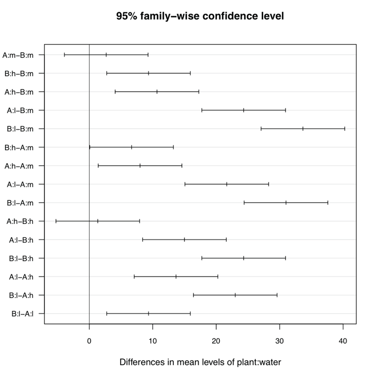
Linear Modeling
Linear modeling is carried out with various commands in R. Various “helper” commands also undertake a variety of useful associated functions.
Command Name
ablineAdds straight lines to a plot. This command can be used to add lines of best fit to fitted models. The command can accept input in various ways:
- Intercept and slope given explicitly
- Intercept and slope taken from fitted-model object
The command can also add vertical or horizontal lines to an existing plot.
Common Usage
abline( a = NULL, b = NULL, reg = NULL, coef = NULL, untf = FALSE, ...)Related Commands
Command Parameters
| a = NULL | The intercept. |
| b = NULL | The slope. |
| reg = NULL | An R object with a coef method. |
| coef = NULL | A vector of length 2, giving the intercept and slope. |
| untf = FALSE | If untf = TRUE, and one or both axes are log-transformed, a curve is drawn corresponding to a line in original coordinates; otherwise, a line is drawn in the transformed coordinate system. |
| ... | Other graphical parameters including col, lty, and lwd. |
Examples
  ## Make data
> count = c(9, 25, 15, 2, 14, 25, 24, 47)
> speed = c(2, 3, 5, 9, 14, 24, 29, 34)

  ## Linear model
> lm1 = lm(count ~ speed)

  ## Plot variables (not shown)
> plot(count ~ speed)

  ## Lines of best fit
> abline(reg = lm1) # From model result
> abline(coef = coef(lm1)) # Coefficients
> abline(a = 8.25, b = 0.79) # Intercept and Slope
Command Name
add1Adds all possible single terms to a model. This command is used to build a model by adding the “best” variable to an existing model. The result shows the AIC value for each possible term. Optionally, you can show a significance statistic.
Common Usage
add1(object, scope, test = "none")Related Commands
Command Parameters
| object | An R object, usually a fitted-model. |
| scope | A formula giving the terms to be considered for adding to the existing model. |
| test = "none" | A character string giving the name of a test statistic to compute for each variable as if it had been added to the original model. The default is "none"; other options are "Chisq" and "F". The F-test is only appropriate for lm and aov models. The Chi-squared test can be an exact test for lm models, or a likelihood ratio test, or test of the reduction in scaled deviance depending on the model type. |
Examples
> data(swiss) # Link to data (in package:datasets)
> names(swiss) # Show variables
[1] "Fertility"        "Agriculture"     "Examination"     "Education"
[5] "Catholic"         "Infant.Mortality"

  ## Build a linear model
  ## Start with "blank" model containing intercept only
> lm1 = lm(Fertility ~ 1, data = swiss)
> lm1

Call:
lm(formula = Fertility ~ 1, data = swiss)

Coefficients:
(Intercept)
      70.14

  ## Evaluate each term to be added to existing model singly
> add1(lm1, scope = swiss, test = "F")
Single term additions

Model:
Fertility ~ 1
                 Df Sum of Sq    RSS    AIC F value     Pr(F)
<none>                        7178.0 238.34
Agriculture       1     894.8 6283.1 234.09  6.4089  0.014917 *
Examination       1    2994.4 4183.6 214.97 32.2087 9.450e-07 ***
Education         1    3162.7 4015.2 213.04 35.4456 3.659e-07 ***
Catholic          1    1543.3 5634.7 228.97 12.3251  0.001029 **
Infant.Mortality  1    1245.5 5932.4 231.39  9.4477  0.003585 **
---
Signif. codes:  0 ‘***’ 0.001 ‘**’ 0.01 ‘*’ 0.05 ‘.’ 0.1 ‘ ‘ 1
Command Name
anovaThis command computes analysis of variance (or deviance) tables for one or more fitted-model objects. You can use this to compare multiple models or to produce the “classic” ANOVA table from a linear model result. Multiple models are compared in the order they are specified (they must be based on the same data set).
Common Usage
anova(object, ...)Related Commands
Command Parameters
| object | An object containing the results obtained by a model fitting such as lm or glm. |
| ... | Additional fitted-model objects. |
Examples
  ## Make data
> height = c(9, 11, 6, 14, 17, 19, 28, 31, 32, 7, 6, 5, 14, 17, 15, 44, 38, 37)
> plant = gl(2, 9, labels = c("vulgaris", "sativa"))
> water = gl(3, 3, 18, labels = c("mid", "hi", "lo"))

  ## Make linear models
> lm1 = lm(height ~ plant + water) # Additive
> lm2 = lm(height ~ plant * water) # Interaction

  ## Make ANOVA tables
> anova(lm1) # Classic ANOVA table
Analysis of Variance Table

Response: height
          Df  Sum Sq Mean Sq F value    Pr(>F)
plant      1   14.22   14.22   1.000    0.3343
water      2 2403.11 1201.56  84.484 1.536e-08 ***
Residuals 14  199.11   14.22
---
Signif. codes:  0 ‘***’ 0.001 ‘**’ 0.01 ‘*’ 0.05 ‘.’ 0.1 ‘ ‘ 1

> anova(lm1, lm2) # Compare models
Analysis of Variance Table

Model 1: height ~ plant + water
Model 2: height ~ plant * water
  Res.Df     RSS Df Sum of Sq      F   Pr(>F)
1     14 199.111
2     12  69.333  2    129.78 11.231 0.001783 **
---
Signif. codes:  0 ‘***’ 0.001 ‘**’ 0.01 ‘*’ 0.05 ‘.’ 0.1 ‘ ‘ 1
Command Name
coef
coefficients
This command extracts model coefficients from fitted-model objects. The coefficients command is an alias for the generic command coef.
Common Usage
coef(object)
coefficients(object)
Related Commands
Command Parameters
| object | An R object that contains coefficients; the result of lm or glm, for example. |
Examples
  ## Make data
> count = c(9, 25, 15, 2, 14, 25, 24, 47)
> speed = c(2, 3, 5, 9, 14, 24, 29, 34)

  ## A linear model
> lm1 = lm(count ~ speed)

  ## The coefficients
> coef(lm1)
(Intercept)       speed
  8.2545956   0.7913603

  ## Produce the same result
> coefficients(lm1)
> lm1$coefficients

> ## Data for ANOVA
> height = c(9, 11, 6, 14, 17, 19, 28, 31, 32, 7, 6, 5, 14, 17, 15, 44, 38, 37)
> plant = gl(2, 9, labels = c("A", "B"))
> water = gl(3, 3, 18, labels = c("m", "h", "l"))

  ## Make an aov object
> aov1 = aov(height ~ plant * water)

  ## The coefficients
> coef(aov1)
  (Intercept)       plantB       waterh       waterl plantB:waterh plantB:waterl
     8.666667    -2.666667     8.000000    21.666667      1.333333     12.000000
Command Name
confintThis command computes confidence intervals for one or more parameters in a fitted-model (for example, resulting from lm or glm).
Common Usage
confint(object, parm, level = 0.95)Related Commands
Command Parameters
| object | A fitted-model object; from lm, for example. |
| parm | A vector of numbers or characters stating which parameters are to be given confidence intervals. If not given, all parameters are used. |
| level = 0.95 | The confidence level required. |
Examples
  ## Make data
> count = c(9, 25, 15, 2, 14, 25, 24, 47)
> speed = c(2, 3, 5, 9, 14, 24, 29, 34)
> algae = c(75, 66, 54, 45, 48, 23, 9, 11)

  ## A linear model
> lm1 = lm(count ~ speed + algae)

  # CI for all terms
> confint(lm1, level = 0.99)
                  0.5 %     99.5 %
(Intercept) -210.594559 128.830182
speed         -2.614892   6.881866
algae         -1.698137   3.100186

  ## CI for only one term
> confint(lm1, parm = "algae")
          2.5 %   97.5 %
algae -0.828495 2.230544
Command Name
drop1This command takes a fitted-model object and removes terms one by one. The result allows you to decide if terms can be dropped from the model as part of a backwards deletion process.
Common Usage
drop1(object, scope, test = "none")Related Commands
Command Parameters
| object | A fitted-model object. |
| scope | A formula giving the terms to be considered for dropping from the existing model. |
| test = "none" | A character string giving the name of a test statistic to compute for each variable as if it had been added to the original model. The default is "none"; other options are "Chisq" and "F". The F-test is only appropriate for lm and aov models. The Chi-squared test can be an exact test for lm models, or a likelihood ratio test, or test of the reduction in scaled deviance depending on the model type. |
Examples
> data(swiss) # Link to data (in package:datasets)
> names(swiss) # Show the variables
[1] "Fertility"        "Agriculture"     "Examination"     "Education"
[5] "Catholic"         "Infant.Mortality"

  ## A linear model, note use of . to denote "everything else"
> lm1 = lm(Fertility ~ ., data = swiss) # A model with all terms

> drop1(lm1, scope = lm1, test = "Chisq")
Single term deletions

Model:
Fertility ~ Agriculture + Examination + Education + Catholic +
    Infant.Mortality
                 Df Sum of Sq    RSS    AIC   Pr(Chi)
<none>                        2105.0 190.69
Agriculture       1    307.72 2412.8 195.10  0.011332 *
Examination       1     53.03 2158.1 189.86  0.279550
Education         1   1162.56 3267.6 209.36 5.465e-06 ***
Catholic          1    447.71 2552.8 197.75  0.002608 **
Infant.Mortality  1    408.75 2513.8 197.03  0.003877 **
---
Signif. codes:  0 ‘***’ 0.001 ‘**’ 0.01 ‘*’ 0.05 ‘.’ 0.1 ‘ ‘ 1
Command Name
familyThis command provides a mechanism to query or specify distribution model parameters for fitted models. The command is used in two main ways:
- To query the distribution model parameters of an object.
- To specify a distribution type in a model such as a generalized linear model via the glm command.
Common Usage
family(object)

binomial(link = "logit")
gaussian(link = "identity")
Gamma(link = "inverse")
inverse.gaussian(link = "1/mu^2")
poisson(link = "log")
quasi(link = "identity", variance = "constant")
quasibinomial(link = "logit")
quasipoisson(link = "log")
Related Commands
Command Parameters
| object | An R object for which you wish to know the distribution model. |
| link | The model link function; usually specified as a character string. |
Examples
  ## Data for glm binomial model
> lat = c(48.1, 45.2, 44.0, 43.7, 43.5, 37.8, 36.6, 34.3)
> a90 = c(47, 177, 1087, 187, 397, 40, 39, 30)
> a100 = c(139, 241, 1183, 175, 671, 14, 17, 0)

  ## Use family to set the distribution type
> glm1 = glm(cbind(a100, a90) ~ lat, family = binomial)

> family(glm1) # Get the distribution family from result

Family: binomial
Link function: logit

  ## A linear model
> lm1 = lm(1:10 ~ c(5:10, 1:4))

> family(lm1) # Get the distribution family

Family: gaussian
Link function: identity
Command Name
fitted
fitted.values
This command extracts model fitted values from objects that are created by modeling commands, for example lm, and glm. The fitted.values command is an alias for the fitted command.
Common Usage
fitted(object)
fitted.values(object)
Related Commands
Command Parameters
| object | An R object that contains fitted values, usually from a command that produces a fitted-model; for example, aov, lm, glm. |
Examples
  ## A binomial generalized linear model (logistic regression)
  ## The data
> lat = c(48.1, 45.2, 44.0, 43.7, 43.5, 37.8, 36.6, 34.3)
> a90 = c(47, 177, 1087, 187, 397, 40, 39, 30)
> a100 = c(139, 241, 1183, 175, 671, 14, 17, 0)

  ## The generalized linear model
> glm1 = glm(cbind(a100, a90) ~ lat, family = binomial)

  ## A linear model
  ## The data
> count = c(9, 25, 15, 2, 14, 25, 24, 47)
> speed = c(2, 3, 5, 9, 14, 24, 29, 34)
> algae = c(75, 66, 54, 45, 48, 23, 9, 11)

  ## The linear model
> lm1 = lm(count ~ speed + algae)

  ## Fitted values
> fitted(glm1)
        1         2         3         4         5         6         7         8
0.7202510 0.6053128 0.5531198 0.5398384 0.5309514 0.2902269 0.2481226 0.1795320
> fitted(lm1)
        1         2         3         4         5         6         7         8
15.961615 11.785882  7.640563  9.865292 22.635800 26.445059 27.298153 39.367636

  ## Access fitted values via model result directly
> glm1$fitted # Same as before
> lm1$fitted  # Same as before
Command Name
glmThis command carries out generalized linear modeling. The modeling can use a variety of distribution functions. The result is a list object with a class attribute "glm".
Common Usage
glm(formula, family = gaussian, data, subset, na.action)Related Commands
Command Parameters
| formula | A formula giving a symbolic description of the model to be fitted. Usually this is in the form response ~ predictor. |
| family = gaussian | A description of the error distribution and link function to be used in the model. This can be specified as a family function or a character string. |
| data | The data frame containing the variables specified in the formula. |
| subset | An optional subset of observations to be used, usually in the form subset = predictor %in% c("a", "b", ...). |
| na.action | A function for handling missing values; defaults to whatever is set in options("na.action"). Usually this is "na.omit", which omits NA items. |
Examples
  ## A Poisson model
> counts <- c(18,17,15,20,10,20,25,13,12)
> outcome <- gl(3,1,9)
> treatment <- gl(3,3)

> glm1 = glm(counts ~ outcome + treatment, family = poisson)
> anova(glm1, test = "Chisq")
Analysis of Deviance Table

Model: poisson, link: log

Response: counts

Terms added sequentially (first to last)


          Df Deviance Resid. Df Resid. Dev P(>|Chi|)
NULL                          8    10.5814
outcome    2   5.4523         6     5.1291   0.06547 .
treatment  2   0.0000         4     5.1291   1.00000
---
Signif. codes:  0 ‘***’ 0.001 ‘**’ 0.01 ‘*’ 0.05 ‘.’ 0.1 ‘ ‘ 1

  ## A binomial generalized linear model (logistic regression)
  ## The data
> lat = c(48.1, 45.2, 44.0, 43.7, 43.5, 37.8, 36.6, 34.3)
> a90 = c(47, 177, 1087, 187, 397, 40, 39, 30)
> a100 = c(139, 241, 1183, 175, 671, 14, 17, 0)

> glm1 = glm(cbind(a100, a90) ~ lat, family = binomial)
> anova(glm1, test = "Chisq")
Analysis of Deviance Table

Model: binomial, link: logit

Response: cbind(a100, a90)

Terms added sequentially (first to last)


     Df Deviance Resid. Df Resid. Dev P(>|Chi|)
NULL                     7    153.633
lat   1   83.301         6     70.333 < 2.2e-16 ***
---
Signif. codes:  0 ‘***’ 0.001 ‘**’ 0.01 ‘*’ 0.05 ‘.’ 0.1 ‘ ‘ 1

  ## A gaussian linear model
  ## The data
> count = c(9, 25, 15, 2, 14, 25, 24, 47)
> speed = c(2, 3, 5, 9, 14, 24, 29, 34)
> algae = c(75, 66, 54, 45, 48, 23, 9, 11)

  ## Same result as lm
> glm1 = glm(count ~ speed + algae, family = gaussian)
> anova(glm1, test = "F")
Analysis of Deviance Table

Model: gaussian, link: identity

Response: count

Terms added sequentially (first to last)


      Df Deviance Resid. Df Resid. Dev      F  Pr(>F)
NULL                      7    1300.88
speed  1   681.36         6     619.51 7.0258 0.04539 *
algae  1   134.62         5     484.90 1.3881 0.29174
---
Signif. codes:  0 ‘***’ 0.001 ‘**’ 0.01 ‘*’ 0.05 ‘.’ 0.1 ‘ ‘ 1
Command Name
lmThis command is used to fit linear models. The model is described in a formula which enables complex models to be symbolized. The lm command is something of a workhorse, and allows regression, analysis of variance, and covariance to be carried out. For some models the aov command is more appropriate; Error terms, for example, are not used in lm. The result of using lm is a list object that has a class attribute "lm".
Common Usage
lm(formula, data, subset, na.action)Related Commands
Command Parameters
| formula | A formula giving a symbolic description of the model to be fitted. Usually this is in the form response ~ predictor. |
| data | The data frame containing the variables specified in the formula. |
| subset | An optional subset of observations to be used, usually in the form subset = predictor %in% c("a", "b", ...). |
| na.action | A function for handling missing values; defaults to whatever is set in options("na.action"). Usually this is "na.omit", which omits NA items. |
Examples
  ## Some data
> count = c(9, 25, 15, 2, 14, 25, 24, 47)  # Response
> speed = c(2, 3, 5, 9, 14, 24, 29, 34)    # Predictor
> algae = c(75, 66, 54, 45, 48, 23, 9, 11) # Predictor

  ## The model
> lm1 = lm(count ~ speed + algae)

> summary(lm1)

Call:
lm(formula = count ~ speed + algae)

Residuals:
     1      2      3      4      5      6      7      8
-6.962 13.214  7.359 -7.865 -8.636 -1.445 -3.298  7.632

Coefficients:
            Estimate Std. Error t value Pr(>|t|)
(Intercept)  -40.882     42.090  -0.971    0.376
speed          2.134      1.178   1.812    0.130
algae          0.701      0.595   1.178    0.292

Residual standard error: 9.848 on 5 degrees of freedom
Multiple R-squared: 0.6273,       Adjusted R-squared: 0.4782
F-statistic: 4.207 on 2 and 5 DF, p-value: 0.08483

> anova(lm1)
Analysis of Variance Table

Response: count
          Df Sum Sq Mean Sq F value  Pr(>F)
speed      1 681.36  681.36  7.0258 0.04539 *
algae      1 134.62  134.62  1.3881 0.29174
Residuals  5 484.90   96.98
---
Signif. codes:  0 ‘***’ 0.001 ‘**’ 0.01 ‘*’ 0.05 ‘.’ 0.1 ‘ ‘ 1
Command Name
resid
residuals
This command extracts residuals from fitted-model objects that have been returned by modeling functions. The residuals command is the generic command and resid is an alias for it.
Common Usage
resid(object)
residuals(object)
Related Commands
Command Parameters
| object | An R object containing residuals; for example, the result from aov, lm, or glm commands. |
Examples
  ## Logistic (binomial) regression
> lat = c(48.1, 45.2, 44.0, 43.7, 43.5, 37.8, 36.6, 34.3)
> a90 = c(47, 177, 1087, 187, 397, 40, 39, 30)
> a100 = c(139, 241, 1183, 175, 671, 14, 17, 0)

  ## The glm
> glm1 = glm(cbind(a100, a90) ~ lat, family = binomial)
> resid(glm1)
         1          2          3          4          5          6          7
 0.8307678 -1.1982004 -3.0582160 -2.1493279  6.4204595 -0.5070130  0.9392368
         8
-3.4456961

> glm1$residuals # Same as resid()

  ## Linear regression
> count = c(9, 25, 15, 2, 14, 25, 24, 47)
> speed = c(2, 3, 5, 9, 14, 24, 29, 34)
> algae = c(75, 66, 54, 45, 48, 23, 9, 11)

  ## The lm
> lm1 = lm(count ~ speed + algae)
> resid(lm1)
        1         2         3         4         5         6         7         8
-6.961615 13.214118  7.359437 -7.865292 -8.635800 -1.445059 -3.298153  7.632364

> lm1$residuals # Same as resid()
Command Name
stepThis command conducts stepwise model building using forwards or backwards algorithms. AIC is used in the decision-making process.
Common Usage
step(object, scope, direction = "both", trace = 1, steps = 1000, k = 2)Related Commands
Command Parameters
| object | An object representing the initial model; this could be a model result or a formula. |
| scope | This defines the range of models to be considered. Usually this is defined using a list that gives the lower and upper models as formulae (see the following examples). |
| direction = "both" | Sets the direction for the model building operation. The default is "both", with "forward" and "backward" as other options. |
| trace = 1 | If trace = 0, no intermediate steps are reported. Setting a value > 1 can give additional information. |
| steps = 1000 | The number of steps to use; the default is 1000. |
| k = 2 | Sets the multiple of the number of degrees of freedom used for the penalty. Use k = 2 (the default) for AIC. Setting k = log(n) equates to BIC (aka SBC). |
| ... | Additional parameters; for example, test (see anova). |
Examples
  ## Make data
> count = c(9, 25, 15, 2, 14, 25, 24, 47)        # Response
> speed = c(2, 3, 5, 9, 14, 24, 29, 34)          # Predictor
> algae = c(75, 66, 54, 45, 48, 23, 9, 11)       # Predictor
> oxyge = c(35, 68, 40, 42, 44, 80, 72, 95)      # Predictor
> lmdat = data.frame(count, speed, algae, oxyge) # Make data frame

 ## Start with intercept and run forwards
  ## Only single term (oxyge) is added
> step(lm(count~1, data = lmdat), scope = list(lower = ~1, upper = lmdat),
 direction = "forward", trace = 1, test = "F")
Start:  AIC=42.73
count ~ 1

        Df Sum of Sq     RSS    AIC F value    Pr(F)
+ oxyge  1   1082.40  218.48 30.458 29.7254 0.001584 **
+ speed  1    681.36  619.51 38.796  6.5990 0.042401 *
+ algae  1    497.67  803.20 40.873  3.7177 0.102108
<none>               1300.88 42.731
---
Signif. codes:  0 ‘***’ 0.001 ‘**’ 0.01 ‘*’ 0.05 ‘.’ 0.1 ‘ ‘ 1

Step:  AIC=30.46
count ~ oxyge

        Df Sum of Sq    RSS    AIC F value  Pr(F)
<none>               218.48 30.458
+ algae  1   14.5897 203.89 31.905  0.3578 0.5758
+ speed  1    0.8597 217.62 32.426  0.0198 0.8937

Call:
lm(formula = count ~ oxyge, data = lmdat)

Coefficients:
(Intercept)        oxyge
   -13.2702       0.5613

> data(swiss)  # Data are in package:datasets
> names(swiss) # View variables (Fertility = response)
[1] "Fertility"        "Agriculture"      "Examination"      "Education"
[5] "Catholic"         "Infant.Mortality"

  ## Start with everything and run backwards
  ## One term is dropped (Examination) from model
> step(lm(Fertility~., data = swiss), scope = list(lower = ~1, upper = swiss),
 direction = "backward", trace = 1, test = "F")
Start:  AIC=190.69
Fertility ~ Agriculture + Examination + Education + Catholic +
    Infant.Mortality

                   Df Sum of Sq    RSS    AIC F value     Pr(F)
- Examination       1     53.03 2158.1 189.86  1.0328  0.315462
<none>                          2105.0 190.69
- Agriculture       1    307.72 2412.8 195.10  5.9934  0.018727 *
- Infant.Mortality  1    408.75 2513.8 197.03  7.9612  0.007336 **
- Catholic          1    447.71 2552.8 197.75  8.7200  0.005190 **
- Education         1   1162.56 3267.6 209.36 22.6432 2.431e-05 ***
---
Signif. codes:  0 ‘***’ 0.001 ‘**’ 0.01 ‘*’ 0.05 ‘.’ 0.1 ‘ ‘ 1

Step:  AIC=189.86
Fertility ~ Agriculture + Education + Catholic + Infant.Mortality

                   Df Sum of Sq    RSS    AIC F value     Pr(F)
<none>                          2158.1 189.86
- Agriculture       1    264.18 2422.2 193.29  5.1413   0.02857 *
- Infant.Mortality  1    409.81 2567.9 196.03  7.9757   0.00722 **
- Catholic          1    956.57 3114.6 205.10 18.6165 9.503e-05 ***
- Education         1   2249.97 4408.0 221.43 43.7886 5.140e-08 ***
---
Signif. codes:  0 ‘***’ 0.001 ‘**’ 0.01 ‘*’ 0.05 ‘.’ 0.1 ‘ ‘ 1

Call:
lm(formula = Fertility ~ Agriculture + Education + Catholic +
    Infant.Mortality, data = swiss)

Coefficients:
     (Intercept)       Agriculture         Education          Catholic
         62.1013           -0.1546           -0.9803            0.1247
Infant.Mortality
          1.0784
Miscellaneous Methods
The analytical methods outlined in this section do not fit easily into the previous categories. The first group of commands deals with clustering. The second group covers ordination, which has foundations in matrix math. The third group covers analytical methods connected with time series. The fourth group covers non-linear modeling.
What’s In This Topic:
- Dissimilarity indices
- Hierarchical clustering
- K-means
- Tree cutting
- Multidimensional scaling (principal coordinates analysis)
- Principal components analysis
- Locally weighted polynomial regression (scatter plot smoothing)
- Non-linear modeling
- Optimization
Clustering
R has a range of commands connected with analytical routines concerned with clustering. These methods include the construction of distance matrices and hierarchical dendrograms as well as k-means analysis.
Command Name
cutreeThis command cuts a tree into groups of data. Generally the tree will have been created by the hclust command. You can specify the number of groups to produce or the cut height(s) to use to cut the tree.
Common Usage
cutree(tree, k = NULL, h = NULL)Related Commands
Command Parameters
| tree | A hierarchical clustering tree object, usually produced by hclust. |
| k = NULL | The number of groups desired. |
| h = NULL | The heights where the tree should be cut. |
Examples
> load("Essential.RData") # Get datafile
> rownames(cd)            # Rows are used as samples
 [1] "ML1" "ML2" "MU1" "MU2" "PL2" "PU2" "SL1" "SL2" "SU1" "SU2"

  ## Create Hierarchical cluster object
> cd.eu = dist(cd, method = "euclidian")     # Distance matrix
> cd.hc = hclust(cd.eu, method = "complete") # Hierarchical cluster

  ## Assign 5 groups and show membership
> cutree(cd.hc, k = 5)
ML1 ML2 MU1 MU2 PL2 PU2 SL1 SL2 SU1 SU2
  1   2   2   1   3   4   4   5   5   5

  ## Show multiple groups.. grp 1 is trivial
> cutree(cd.hc, k = 1:5)
    1 2 3 4 5
ML1 1 1 1 1 1
ML2 1 1 2 2 2
MU1 1 1 2 2 2
MU2 1 1 1 1 1
PL2 1 2 3 3 3
PU2 1 1 2 2 4
SL1 1 1 2 2 4
SL2 1 2 3 4 5
SU1 1 2 3 4 5
SU2 1 2 3 4 5

> cd.hc$height # View cut heights
[1] 11.46996 15.22104 15.63458 16.20247 16.90444 21.83941 22.11063 26.38863
[9] 26.81567

  ## Select height and show membership
> cutree(cd.hc, h = 20)
ML1 ML2 MU1 MU2 PL2 PU2 SL1 SL2 SU1 SU2
  1   2   2   1   3   4   4   5   5   5
Command Name
distThis command computes distance matrices (that is, dissimilarity). Various algorithms can be used (see the following command parameters). The result is an object with a class attribute "dist". There is a dedicated print routine for "dist" objects.
Common Usage
dist(x, method = "euclidian", diag = FALSE, upper = FALSE, p = 2)Related Commands
Command Parameters
| x | Numerical data in a data frame or matrix. |
| method = "euclidian" | The method used to generate the distances; the default is "euclidian". Other options are "maximum", "manhattan", "canberra", "binary", and "minkowski". |
| diag = FALSE | If diag = TRUE, the diagonal of the matrix is given. This actually sets an attribute of the result so it is possible to create a "dist" object with diag = FALSE but use print with diag = TRUE (see the following examples). |
| upper = FALSE | If upper = TRUE, the upper quadrant is given (in addition to the lower). This sets an attribute of the result so it is possible to create a "dist" object with one setting and print the opposite. |
| p = 2 | The power of the Minkowski distance. |
Examples
> load("Essential.RData") # Get datafile
> rownames(cd)            # Rows are used as samples
 [1] "ML1" "ML2" "MU1" "MU2" "PL2" "PU2" "SL1" "SL2" "SU1" "SU2"

  ## Use Euclidian algorithm
> cd.eu = dist(cd, method = "euclidian")
> print(cd.eu, digits = 4) # Show the result
      ML1   ML2   MU1   MU2   PL2   PU2   SL1   SL2   SU1
ML2 21.82
MU1 20.42 16.90
MU2 15.63 22.35 24.73
PL2 26.34 21.78 23.21 25.90
PU2 21.84 18.64 21.61 26.39 23.17
SL1 25.12 19.89 21.84 25.20 19.01 15.22
SL2 21.14 21.25 22.47 21.86 18.46 19.52 17.62
SU1 26.35 24.85 26.13 26.82 20.83 23.59 19.58 16.20
SU2 24.45 25.79 26.39 25.49 22.11 23.45 21.38 11.47 13.12

  ## Use Binary algorithm
> cd.bn = dist(cd, method = "binary", upper = TRUE, diag = TRUE)
> print(cd.bn, digits = 2, diag = FALSE)
     ML1  ML2  MU1  MU2  PL2  PU2  SL1  SL2  SU1  SU2
ML1      0.59 0.50 0.55 0.92 0.76 0.93 0.92 0.95 0.95
ML2 0.59      0.46 0.42 0.84 0.77 0.86 0.89 0.87 0.95
MU1 0.50 0.46      0.48 0.87 0.72 0.88 0.88 0.86 0.91
MU2 0.55 0.42 0.48      0.88 0.81 0.89 0.91 0.92 0.97
PL2 0.92 0.84 0.87 0.88      0.80 0.79 0.81 0.82 0.89
PU2 0.76 0.77 0.72 0.81 0.80      0.83 0.87 0.88 0.88
SL1 0.93 0.86 0.88 0.89 0.79 0.83      0.75 0.66 0.80
SL2 0.92 0.89 0.88 0.91 0.81 0.87 0.75      0.69 0.75
SU1 0.95 0.87 0.86 0.92 0.82 0.88 0.66 0.69      0.61
SU2 0.95 0.95 0.91 0.97 0.89 0.88 0.80 0.75 0.61
Command Name
hclustThis command carries out hierarchical clustering. The command takes a matrix of distances (dissimilarity) and creates an object with a class attribute "hclust". There is a special version of the plot command for "hclust" objects; see the following examples.
Common Usage
hclust(d, method = "complete")Related Commands
Command Parameters
| d | A dissimilarity matrix; usually this is produced by the dist command. |
| method = "complete" | The method of agglomeration to be used; the default is "complete", with other options being "ward", "single", "average", "mcquitty", "median", and "centroid". |
Examples
> load("Essential.RData") # Get datafile
> rownames(cd)            # Rows are used as samples
 [1] "ML1" "ML2" "MU1" "MU2" "PL2" "PU2" "SL1" "SL2" "SU1" "SU2"

  ## Create Hierarchical cluster object
> cd.eu = dist(cd, method = "euclidian")     # Distance matrix

> cd.hc = hclust(cd.eu, method = "complete") # Hierarchical cluster
> cd.hc        # The result

Call:
hclust(d = cd.eu, method = "complete")

Cluster method   : complete
Distance         : euclidean
Number of objects: 10

> names(cd.hc) # Show result components
[1] "merge" "height" "order" "labels" "method" "call"
[7] "dist.method"
## Use plot to create dendrogram (Figure 2-3)
> plot(cd.hc)Figure 2-3: Dendrogram of hierarchical cluster analysis
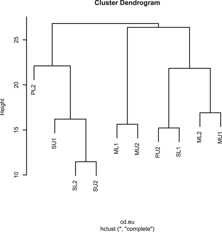
Command Name
kmeansThis command carries out k-means clustering on a data matrix.
Common Usage
kmeans(x, centers, iter.max = 10, nstart = 1, algorithm = "Hartigan-Wong")Related Commands
Command Parameters
| x | An R object containing numeric data; usually this is a matrix or data frame. |
| centers | Either the number of clusters required or a set of initially distinct cluster centers. If this is a single number, a random set of distinct rows in x is chosen as the initial centers. |
| iter.max = 10 | The maximum number of iterations allowed. |
| nstart = 1 | Used for the random selection of centers to start. Setting a value > 1 can be helpful when differentiating between clusters. |
| algorithm = "Hartigan-Wong" | Sets the algorithm to use for the analysis; the default is "Hartigan-Wong", but other options are "Lloyd", "Forgy", and "MacQueen". |
Examples
  ## Some data for k-means analysis
> data(iris)  # Morphological data for 3 putative species
> names(iris) # See variables
[1] "Sepal.Length" "Sepal.Width"  "Petal.Length" "Petal.Width"  "Species"

  ## K-means with 3 clusters (there are 3 putative species)
  ## Use columns 1:4 as data (column 5 is species labels/names)
> iris.k = kmeans(iris[,1:4], centers = 3)
> iris.k # Show result
K-means clustering with 3 clusters of sizes 38, 62, 50

Cluster means:
  Sepal.Length Sepal.Width Petal.Length Petal.Width
1     6.850000    3.073684     5.742105    2.071053
2     5.901613    2.748387     4.393548    1.433871
3     5.006000    3.428000     1.462000    0.246000

Clustering vector:
  [1] 2 2 2 2 2 2 2 2 2 2 2 2 2 2 2 2 2 2 2 2 2 2 2 2 2 2 2 2 2 2 2 2 2 2 2 2
 [37] 2 2 2 2 2 2 2 2 2 2 2 2 2 2 1 1 3 1 1 1 1 1 1 1 1 1 1 1 1 1 1 1 1 1 1 1
 [73] 1 1 1 1 1 3 1 1 1 1 1 1 1 1 1 1 1 1 1 1 1 1 1 1 1 1 1 1 3 1 3 3 3 3 1 3
[109] 3 3 3 3 3 1 1 3 3 3 3 1 3 1 3 1 3 3 1 1 3 3 3 3 3 1 3 3 3 3 1 3 3 3 1 3
[145] 3 3 1 3 3 1

Within cluster sum of squares by cluster:
[1] 23.87947 39.82097 15.15100
 (between_SS / total_SS =  88.4 %)

Available components:

[1] "cluster"      "centers"      "totss"        "withinss"     "tot.withinss"
[6] "betweenss"    "size"

  ## Visualize using two of the morphological variables (Figure 2-4)
> plot(iris[, c(1,4)], pch = iris.k$cluster) # Clusters with different points

  ## Add centers
> points(iris.k$centers[, c(1,4)], pch = 8, cex = 2)  # Asterisk
> points(iris.k$centers[, c(1,4)], pch = 20, cex = 2) # Solid circle
## Show group membership
> table(iris$Species, iris.k$cluster)
1 2 3
setosa 0 0 50
versicolor 2 48 0
virginica 36 14 0Figure 2-4: K-means cluster analysis for Iris morphological data

Ordination
There are two main kinds of ordination built into the base distribution of R. Principal components analysis (PCA) is a method of dealing with multivariate data. Two commands carry out PCA: prcomp and princomp. The commands use slightly different mathematical approaches. Classical multidimensional scaling (also called principal coordinates analysis) is conducted via the cmdscale command.
Command Name
cmdscaleThis command carries out classical multidimensional scaling, which is also known as principal coordinates analysis. The command takes a set of dissimilarities (see dist), and returns a set of points as x, y, coordinates. The distance between the points is broadly equal to the dissimilarities. The result is a matrix object with columns [1] and [2] that are analogous to the x and y coordinates, respectively. Additional dimensions can be specified in the command, so extra columns may result.
Common Usage
cmdscale(d, k = 2, eig = FALSE, add = FALSE, x.ret = FALSE)Related Commands
Command Parameters
| d | A dissimilarity matrix; usually created with the dist command. |
| k = 2 | The dimensions of the result to return. Usually k = 2 is sufficient but additional columns of coordinates can be returned by increasing the value of k. |
| eig = FALSE | If TRUE, the eigenvalues are computed and returned as part of the result. |
| add = FALSE | If TRUE, an additive constant c* is computed. This is added to all non-diagonal dissimilarities such that all n-1 eigenvalues are non-negative. |
| x.ret = FALSE | If TRUE, the doubly centered symmetric distance matrix is returned. |
Examples
> load(file = "Essential.RData") # Load file

  ## View row names (the data samples)
> rownames(moss)
[1] "BN2" "LT1" "LT2" "PE3" "PO2" "PT1" "PT3" "QA1" "QR1"

  ## Create dissimilarity matrix using Euclidian algorithm
> moss.eu = dist(moss, method = "euclidian")

  ## Simplest default multidimensional scaling
> moss.pco = cmdscale(moss.eu)

  ## Result is simple matrix. Columns can be used as basis for plot
> moss.pco
           [,1]        [,2]
BN2  -0.4446475  34.8789419
LT1 -18.1046921   2.8738551
LT2 -22.5535658  -0.1146282
PE3  39.2108396  -2.0936131
PO2 -29.1878891 -13.1531653
PT1  31.1197817   3.1753791
PT3  45.2687047 -13.5379996
QA1 -24.0843294  -7.6439190
QR1 -21.2242021  -4.3848508

  ## If additional parameters are specified the result is a list
  ## Distance coordiantes $points
  ## Eigenvalues $eig
  ## Goodness of Fit of eigenvalues $GOF

> moss.pco = cmdscale(moss.eu, k = 2, eig = TRUE)
> moss.pco
$points
           [,1]        [,2]
BN2  -0.4446475  34.8789419
LT1 -18.1046921   2.8738551
LT2 -22.5535658  -0.1146282
PE3  39.2108396  -2.0936131
PO2 -29.1878891 -13.1531653
PT1  31.1197817   3.1753791
PT3  45.2687047 -13.5379996
QA1 -24.0843294  -7.6439190
QR1 -21.2242021  -4.3848508

$eig
[1] 7.274282e+03 1.673219e+03 4.010192e+02 3.237306e+02 1.945114e+02
[6] 5.300512e+01 3.839127e+01 1.849303e+01 9.928362e-13

$x
NULL

$ac
[1] 0

$GOF
[1] 0.896844 0.896844
Command Name
prcompThis command carries out principal components analysis on a data matrix. The result is an object with a class attribute "prcomp". The PCA is carried out using svd, which is a slightly different approach to the princomp command. There is a special plotting command for the result, biplot. The command can accept input using a formula.
Common Usage
prcomp(formula, data = NULL, subset, na.action,
       retx = TRUE, center = TRUE, scale = FALSE, tol = NULL)
Related Commands
Command Parameters
| formula | A formula with no response variable, e.g., of the form ~ predictor. The variables should be numeric. Alternatively the formula can be a numeric matrix or data frame. |
| data = NULL | An optional data frame that contains the variables in the formula. |
| subset | An optional vector giving the rows to use from the data matrix. |
| na.action | A function that details what to do with NA items. The default is usually na.omit, which omits missing data. |
| retx = TRUE | By default the rotated variables are returned in the result object. |
| center = TRUE | If TRUE, the variables are shifted to be zero centered. You can also give a vector of length equal to the number of variables (columns in the data matrix). |
| scale = FALSE | If scale = TRUE, the variables are scaled to have unit variance before the analysis (this is generally advisable). You can also give a vector of length equal to the number of variables (columns in the data matrix). |
| tol = NULL | A value indicating the magnitude below which components should be omitted; this equates to the product of tol and the standard deviation of first component. |
Examples
  ## Use datasets:USArrests
> data(USArrests)  # Get datafile
> names(USArrests) # View variable names
[1] "Murder"   "Assault"  "UrbanPop" "Rape"

  ## Scaled PCA using entire data.frame
> pca1 = prcomp(USArrests, scale = TRUE)

  ## Both following commands produce same PCA as previous
> pca2 = prcomp(~., data = USArrests, scale = TRUE)
> pca3 = prcomp(~ Murder + Assault + Rape + UrbanPop,
 data = USArrests, scale = TRUE)

> pca1 # View result
Standard deviations:
[1] 1.5748783 0.9948694 0.5971291 0.4164494

Rotation:
                PC1        PC2        PC3         PC4
Murder   -0.5358995  0.4181809 -0.3412327  0.64922780
Assault  -0.5831836  0.1879856 -0.2681484 -0.74340748
UrbanPop -0.2781909 -0.8728062 -0.3780158  0.13387773
Rape     -0.5434321 -0.1673186  0.8177779  0.08902432

> names(pca1) # View elements in result object
[1] "sdev"     "rotation" "center"   "scale"    "x"

> summary(pca1) # Summary
Importance of components:
                         PC1    PC2     PC3     PC4
Standard deviation     1.575 0.9949 0.59713 0.41645
Proportion of Variance 0.620 0.2474 0.08914 0.04336
Cumulative Proportion  0.620 0.8675 0.95664 1.00000

  ## Plots for results...
  ## Scree-plot of variances (Figure 2-5)
> plot(pca1, type = "lines", main = "PCA for USArrests")
Figure 2-5: Scree-plot of variances from principal components analysis

  ## Bi-plot of result (Figure 2-6)
> biplot(pca1, col = 1, cex = c(0.8, 1.2), expand = 0.9)
Figure 2-6: Bi-plot of principal components analysis

Command Name
princompThis command carries out principal components analysis on a data matrix. The result is an object with a class attribute "princomp". The PCA is carried out using eigen, which is a slightly different approach to the prcomp command (the prcomp approach is generally preferable). The biplot plotting command is used for the result. The command can accept input using a formula.
Common Usage
princomp(formula, data = NULL, subset, na.action, cor = FALSE,
         scores = TRUE, covmat = NULL
Related Commands
Command Parameters
| formula | A formula with no response variable, e.g., of the form ~ predictor. The variables should be numeric. Alternatively, the formula can be a numeric matrix or data frame. |
| data = NULL | An optional data frame that contains the variables in the formula. |
| subset | An optional vector giving the rows to use from the data matrix. |
| na.action | A function that details what to do with NA items. The default is usually na.omit, which omits missing data. |
| cor = FALSE | If cor = TRUE, the correlation matrix is used (only if no constant variables exist); the default is to use the covariance matrix. Using cor = TRUE is equivalent to scale = TRUE in the prcomp command. |
| scores = TRUE | If TRUE (the default), the score on each principal component is calculated. |
| covmat = NULL | A covariance matrix. If supplied, this is used instead of calculating it from the data given. |
Examples
  ## Use datasets:USArrests
> data(USArrests)  # Get datafile
> names(USArrests) # View variable names
[1] "Murder"   "Assault"  "UrbanPop" "Rape"

> pca1 = princomp(USArrests, cor = TRUE)

  ## Both following commands produce same PCA as previous
> pca2 = princomp(~., data = USArrests, cor = TRUE)
> pca3 = princomp(~ Murder + Assault + Rape + UrbanPop,
 data = USArrests, cor = TRUE)

> pca1 # View result
Call:
princomp(x = USArrests, cor = TRUE)

Standard deviations:
   Comp.1    Comp.2    Comp.3    Comp.4
1.5748783 0.9948694 0.5971291 0.4164494

 4  variables and  50 observations.

> names(pca1) # View elements in result object
[1] "sdev"   "loadings" "center"   "scale"   "n.obs"   "scores"   "call"

> summary(pca1) # Summary
Importance of components:
                          Comp.1    Comp.2    Comp.3     Comp.4
Standard deviation     1.5748783 0.9948694 0.5971291 0.41644938
Proportion of Variance 0.6200604 0.2474413 0.0891408 0.04335752
Cumulative Proportion  0.6200604 0.8675017 0.9566425 1.00000000

  ## Plots for results...
  ## Scree-plot of variances (refer to Figure 2-5)
> plot(pca1, type = "lines", main = "PCA for USArrests")

  ## Bi-plot of data (refer to Figure 2-6)
> biplot(pca1, col = 1, cex = c(0.8, 1.2), expand = 0.9)
Time Series
This section shows commands related to time-series data.
Command Name
Box.testThis command carries out Box-Pierce or Ljung-Box tests for examining independence in time series. These tests are also called “portmanteau” tests. The result is a list with a class attribute "htest".
Common Usage
Box.test(x, lag = 1, type = "Box-Pierce", fitdf = 0)Related Commands
Command Parameters
| x | A numeric vector or a univariate time-series object. |
| lag = 1 | The lag to use for the autocorrelation coefficients. |
| type = "Box-Pierce" | The test to carry out; defaults to "Box-Pierce" with "Ljung-Box" as an alternative. You can use an abbreviation. |
| fitdf = 0 | The number of degrees of freedom to be subtracted if x is a series of residuals. |
Examples
> data(lynx) # Canadian annual lynx trapped

> Box.test(lynx, lag = 1, type = "Box-Pierce")

       Box-Pierce test

data:  lynx
X-squared = 57.6, df = 1, p-value = 3.209e-14

> Box.test(lynx, lag = 1, type = "Ljung-Box")

       Box-Ljung test

data:  lynx
X-squared = 59.1292, df = 1, p-value = 1.477e-14
Command Name
PP.testThis command carries out the Phillips-Perron test for the null hypothesis that x has a unit root against a stationary alternative. The result is a list with a class attribute "htest".
Common Usage
PP.test(x, lshort = TRUE)Related Commands
Command Parameters
| x | A numeric vector or a univariate time series. |
| lshort = TRUE | If TRUE (the default), the short version of the truncation lag parameter is used. |
Examples
> data(lynx) # Canadian annual lynx trapped
> PP.test(lynx)
Phillips-Perron Unit Root Test
data: lynx
Dickey-Fuller = -4.5852, Truncation lag parameter = 4, p-value = 0.01
> set.seed(55) # Set random number seed
> x = rnorm(1000) # Make 1000 random values from normal distribution
> PP.test(x)
Phillips-Perron Unit Root Test
data: x
Dickey-Fuller = -31.4208, Truncation lag parameter = 7, p-value = 0.01
> y = cumsum(x) # This should have unit root
> PP.test(y)
Phillips-Perron Unit Root Test
data: y
Dickey-Fuller = -0.8208, Truncation lag parameter = 7, p-value = 0.9598Non-linear Modeling and Optimization
In non-linear modeling the observed data are modeled by a function that does not necessarily conform to a strict linear pattern. The technique of non-linear modeling uses successive approximations to fit the model.
In a similar vein, locally weighted polynomial regression is a method often used to visualize relationships by fitting a kind of best-fit line. Rather than being straight, the line is “influenced” by the points it passes by. It is often called scatter plot smoothing.
Command Name
loessThis command carries out local polynomial regression fitting. A common use for this is to produce a locally fitted model that can be added to a scatter plot as a trend line to help visualize the relationship. The trend line is not a straight line but weaves through the scatter of points; thus loess is often referred to as a scatter plot smoother.
Common Usage
loess(formula, data, weights, subset, na.action,
model = FALSE, span = 0.75, degree = 2, family = "gaussian")Related Commands
Command Parameters
| formula | A formula that describes the regression. You specify the response and up to four numeric predictors. The formula is usually of the form response ~ p1 * p2 * p3 * p4, but additive predictors are allowed. |
| data | A data frame specifying where the variables in the formula are to be found. |
| weights | Optional weights for each case; usually specified as a vector. |
| subset | A subset of observations, usually of the form subset = group %in% c("a", "b", ...). |
| na.action | A function indicating what to do if NA items are present. The default is na.omit, which omits the NA items. |
| model = FALSE | If TRUE, the model frame is returned as part of the result (essentially the original data). |
| span = 0.75 | A numerical value that controls the degree of smoothing. Smaller values result in less smoothing. |
| degree = 2 | The degree of the polynomials to use; this is normally 1 or 2. |
| family = "gaussian" | The kind of fitting carried out. The default, "gaussian", uses least-squares. The alternative, "symmetric", uses a re-descending M estimator with Tukey’s biweight function. |
Examples
## Use cars data from R datasets
> data(cars) # Make sure data are ready
## Make a local ploynomial regression
> cars.loess = loess(dist ~ speed, data = cars)
## View the result (a summary)
> cars.loess
Call:
loess(formula = dist ~ speed, data = cars)
Number of Observations: 50
Equivalent Number of Parameters: 4.78
Residual Standard Error: 15.29
## Look at names of items in result
> names(cars.loess)
[1] "n" "fitted" "residuals" "enp" "s" "one.delta"
[7] "two.delta" "trace.hat" "divisor" "pars" "kd" "call" [13] "terms" "xnames" "x" "y" "weights"
## Make a basic scatter plot of the original data (Figure 2-7)
> plot(cars)
## Add loess line
> lines(cars.loess$x, cars.loess$fitted, lwd = 3)
## Give a title
> title(main = "loess smoother")Figure 2-7: Two forms of scatter plot smoother compared

Command Name
lowessThis command carries out scatter plot smoothing. The algorithm uses a locally weighted polynomial regression. A common use for this is to produce a locally fitted model that can be added to a scatter plot as a trend line to help visualize the relationship.
Common Usage
lowess(x, y = NULL, f = 2/3, iter = 3,
delta = 0.01 * diff(range(xy$x[o])))Related Commands
Command Parameters
| x, y = NULL | Vectors that give the coordinates of the points in the scatter plot. Alternatively, if x is an object with a plotting structure (that is, it contains x and y components) then y can be missing. |
| f = 2/3 | Controls the smoothness by giving the proportion of points in the plot that influence the smoothing at each value. Larger values result in smoother curves. |
| iter = 3 | The number of iterations performed; this helps robustness of the result. Larger values take more computing power and run slower. |
| delta | Allows the computation to speed up at the expense of some smoothness. The default value is 1/100 of the range of x. Instead of computing the local polynomial fit for each point, some points are skipped and interpolation is used. Larger values result in more interpolation. |
Examples
## Use cars data from R datasets (built into R)> data(cars) # Make sure data are ready
## Make a local ploynomial regression
> cars.lowess = lowess(cars$speed, cars$dist)
> cars.lowess # Result contains x and y elements
$x
[1] 4 4 7 7 8 9 10 10 10 11 11 12 12 12 12 13 13 13 13 14 14 14 14 15
[25] 15 15 16 16 17 17 17 18 18 18 18 19 19 19 20 20 20 20 20 22 23 24 24 24
[49] 24 25
$y
[1] 4.965459 4.965459 13.124495 13.124495 15.858633 18.579691 21.280313
[8] 21.280313 21.280313 24.129277 24.129277 27.119549 27.119549 27.119549
[15] 27.119549 30.027276 30.027276 30.027276 30.027276 32.962506 32.962506
[22] 32.962506 32.962506 36.757728 36.757728 36.757728 40.435075 40.435075
[29] 43.463492 43.463492 43.463492 46.885479 46.885479 46.885479 46.885479
[36] 50.793152 50.793152 50.793152 56.491224 56.491224 56.491224 56.491224
[43] 56.491224 67.585824 73.079695 78.643164 78.643164 78.643164 78.643164
[50] 84.328698
## Make a basic scatter plot of the original data (refer to Figure 2-7)
> plot(cars)
## Add lowess line
> lines(cars.lowess, lwd = 3)
## Add graph title
> title(main = "lowess smoother")Command Name
nlmThis command carries out a minimization of a function using a Newton-type algorithm.
Common Usage
nlm(f, p, ..., hessian = FALSE, print.level = 0)Related Commands
Command Parameters
| f | The function to be minimized. |
| p | The starting parameter values for the minimization. |
| ... | Additional arguments to f. |
| hessian = FALSE | If hessian = TRUE, the hessian of f at the minimum is returned. |
| print.level = 0 | Controls the information shown through the minimization process: if 0, no information is shown; if 1, only initial and final details are shown; if 2, all tracing information through the iteration process is shown. |
Examples
## Make a simple function to minimize
> f = function(x, a) sum((x-a)^2)
> nlm(f, p = c(6, 9), a = c(2, 4), hessian = TRUE)
$minimum
[1] 5.482287e-26
$estimate
[1] 2 4
$gradient
[1] 3.659295e-13 -2.917666e-13
$hessian
[,1] [,2]
[1,] 2.000000e+00 8.271806e-17
[2,] 8.271806e-17 2.000000e+00
$code
[1] 1
$iterations
[1] 2Command Name
nlsThis command carries out non-linear regression; it determines the non-linear (weighted) least-squares estimates of the parameters of a given model. The result is a list with a class attribute "nls".
Common Usage
nls(formula, data, start, algorithm, trace, subset, weights, na.action)Related Commands
Command Parameters
| formula | A formula for the non-linear model, which should include variables and parameters. |
| data | A data frame that contains the variables in the formula. |
| start | Starting estimates, given as a list. |
| algorithm | A character string that gives the algorithm to be used. The default is a Gauss-Newton algorithm; options are "default", "plinear", and "port". |
| trace = FALSE | If trace = TRUE, the iteration process is displayed. |
| subset | An optional subset of the data set. |
| weights | An optional vector of fixed weights. If present, the objective function is weighted least squares. |
| na.action | A function indicating what to do if NA items are present. The default is na.omit, which omits the NA items. |
Examples
## Make data (substrate concentration and rate of reaction)
> conc = c(1, 1.5, 2, 2.7, 5, 7.7, 10)
> vel = c(9, 12.5, 16.7, 20, 28.6, 37, 38.5)
> mm = data.frame(conc, vel)
## Fit a Michaelis Menten model
> mm.nlm = nls(vel ~ Vm * conc / (K + conc), data = mm,
start = list(K = 1, Vm = 1))
> coef(mm.nlm) # The coefficients
K Vm
5.602863 61.518487
## Plot model (see Figure 2-8)
> plot(vel ~ conc, data = mm, type = "b") # Original data
> lines(spline(mm$conc, fitted(mm.nlm)), lwd = 3) # Add fitted curveFigure 2-8: Plot of a Michaelis-Menten model using non-linear modeling (nls)
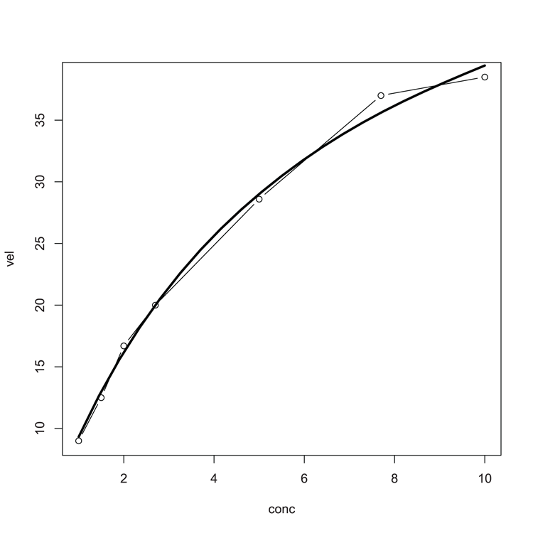
## using a selfStart model
## More data
> data(DNase) # Get data from datasets
> DNase1 <- subset(DNase, Run == 1) # Use only part of data
## The model
> fm1DNase1 <- nls(density ~ SSlogis(log(conc), Asym, xmid, scal), DNase1)
> summary(fm1DNase1)
Formula: density ~ SSlogis(log(conc), Asym, xmid, scal)
Parameters:
Estimate Std. Error t value Pr(>|t|)
Asym 2.34518 0.07815 30.01 2.17e-13 ***
xmid 1.48309 0.08135 18.23 1.22e-10 ***
scal 1.04146 0.03227 32.27 8.51e-14 ***
---
Signif. codes: 0 ‘***’ 0.001 ‘**’ 0.01 ‘*’ 0.05 ‘.’ 0.1 ‘ ‘ 1
Residual standard error: 0.01919 on 13 degrees of freedom
Number of iterations to convergence: 0
Achieved convergence tolerance: 3.281e-06
> coef(fm1DNase1) # Get coefficients only
Asym xmid scal
2.345180 1.483090 1.041455Command Name
optimThis command carries out general-purpose optimization based on Nelder–Mead, quasi-Newton, and conjugate-gradient algorithms. It includes an option for box-constrained optimization and simulated annealing.
Common Usage
optim(par, fn, gr = NULL, ..., method = "Nelder-Mead",
lower = -Inf, upper = Inf, control = list(), hessian = FALSE)Related Commands
Command Parameters
| par | Initial values for the parameters to be optimized. |
| fn | A function to be minimized (or maximized); the first argument must be a vector of parameters over which the minimization is to take place. |
| gr = NULL | A function to return the gradient. |
| ... | Additional arguments to pass to fn and gr. |
| method = "Nelder-Mead" | The method for the optimization. The default is "Nelder-Mead". Other options are "BFGS", "CG", "L-BFGS-B", and "SANN". |
| lower = -Inf | Lower bound on the variables for the "L-BFGS-B" method. |
| upper = Inf | Upper bound on the variables for the "L-BFGS-B" method. |
| control = list() | A list of control parameters. |
| hessian = FALSE | If TRUE, a differentiated Hessian matrix is returned. |
Examples
# Make a simple function to optimize
> f = function(x, a) sum((x-a)^2)
> optim(c(6, 9), f, a = c(2, 4), hessian = TRUE)
$par
[1] 1.999964 4.000290
$value
[1] 8.549353e-08
$counts
function gradient
63 NA
$convergence
[1] 0
$message
NULL
$hessian
[,1] [,2]
[1,] 2.000000e+00 -8.131516e-17
[2,] -8.131516e-17 2.000000e+00Command Name
optimise
optimizeThese commands carry out one-dimensional optimization. The optimise command is simply an alias for optimize. The command searches a given interval, from the lower end to the upper, for a minimum or maximum of a given function with respect to its first argument.
Common Usage
optimize(f, interval, ...,
lower = min(interval), upper = max(interval),
maximum = FALSE, tol = .Machine$double.eps^0.25)Related Commands
Command Parameters
| f | The function to be optimized. The function is either minimized or maximized over its first argument depending on the value of maximum. |
| interval | A vector that gives the endpoints of the interval to be searched for the minimum. |
| ... | Additional arguments to be passed to the function, f. |
| lower = min(interval) | The lower end point of the interval to be searched. |
| upper = max(interval) | The upper end point of the interval to be searched. |
| maximum = FALSE | If maximum = TRUE, the function is maximized rather than minimized. |
| tol | A value for the accuracy. |
Examples
## Make a simple function to optimize
> f = function(x, a) sum((x-a)^2)
> optimize(f, interval = c(6, 9), a = c(2, 4))
$minimum
[1] 6.000076
$objective
[1] 20.00091
> optimize(f, interval = c(6, 9), a = c(2, 4), maximum = TRUE)
$maximum
[1] 8.999924
$objective
[1] 73.99818Command Name
polyrootThis command finds zeros of real or complex polynomials using the Jenkins-Traub algorithm.
Common Usage
polyroot(z)Related Commands
Command Parameters
| z | A vector of polynomial coefficients in increasing order. |
Examples
> polyroot(c(4, 2))
[1] -2+0i
> polyroot(c(4, 2, 3))
[1] -0.333333+1.105542i -0.333333-1.105542i
> polyroot(c(4, 2, 3, 2))
[1] 0.068000+1.103572i -1.635999+0.000000i 0.068000-1.103572iCommand Name
SSlogisThis command creates self-starting non-linear models. The command evaluates the logistic function and its gradient, which creates starting estimates for the parameters.
Common Usage
SSlogis(input, Asym, xmid, scal)Related Commands
Command Parameters
| input | A numeric vector of values used to evaluate the model. |
| Asym | A numeric value representing the asymptote. |
| xmid | A numeric value representing the x value at the inflection point of the curve. |
| scal | A value for the scale parameter. |
Examples
> data(DNase) # Data from datasets
> DNase1 <- subset(DNase, Run == 1) # Use only part of the data
## A self-starting non-linear model
> fm1DNase1 <- nls(density ~ SSlogis(log(conc), Asym, xmid, scal), DNase1)
> coef(fm1DNase1)
Asym xmid scal
2.345180 1.483090 1.041455
## Estimate starting values
> SSlogis(log(DNase1$conc), Asym = 2.5, xmid = 1.5, scal = 1) # Response only
[1] 0.02694401 0.02694401 0.10440049 0.10440049 0.20043094 0.20043094
[7] 0.37110918 0.37110918 0.64628190 0.64628190 1.02705657 1.02705657
[13] 1.45596838 1.45596838 1.84021742 1.84021742
> Asym = 2.5; xmid = 1.5; scal = 1 # Set values
## Use set values
> SSlogis(log(DNase1$conc), Asym, xmid, scal) # Response and gradient
[1] 0.02694401 0.02694401 0.10440049 0.10440049 0.20043094 0.20043094
[7] 0.37110918 0.37110918 0.64628190 0.64628190 1.02705657 1.02705657
[13] 1.45596838 1.45596838 1.84021742 1.84021742
attr(,"gradient")
Asym xmid scal
[1,] 0.01077760 -0.02665362 0.1204597
[2,] 0.01077760 -0.02665362 0.1204597
[3,] 0.04176020 -0.10004070 0.3134430
[4,] 0.04176020 -0.10004070 0.3134430
[5,] 0.08017238 -0.18436192 0.4498444
[6,] 0.08017238 -0.18436192 0.4498444
[7,] 0.14844367 -0.31602037 0.5520434
[8,] 0.14844367 -0.31602037 0.5520434
[9,] 0.25851276 -0.47920978 0.5049495
[10,] 0.25851276 -0.47920978 0.5049495
[11,] 0.41082263 -0.60511849 0.2181850
[12,] 0.41082263 -0.60511849 0.2181850
[13,] 0.58238735 -0.60803081 -0.2022198
[14,] 0.58238735 -0.60803081 -0.2022198
[15,] 0.73608697 -0.48565736 -0.4981527
[16,] 0.73608697 -0.48565736 -0.4981527Command Name
unirootThis command carries out one-dimensional root (zero) finding. It searches the given interval from the lower to the upper to find a root (zero) of the given function, with respect to its first argument.
Common Usage
uniroot(f, interval, ..., lower = min(interval), upper = max(interval),
tol = .Machine$double.eps^0.25, maxiter = 1000)Related Commands
Command Parameters
| f | The function for which the root is required. |
| interval | A vector that gives the endpoints of the interval to be searched for the root. |
| ... | Additional arguments to be passed to the function, f. |
| lower = min(interval) | The lower end point of the interval to be searched. |
| upper = max(interval) | The upper end point of the interval to be searched. |
| tol | A value for the accuracy. |
| maxiter = 1000 | The maximum number of iterations. |
Examples
## Make a function
> f = function (x, a) x – a
## Find root
> uniroot(f, interval = c(0, 1), a= 0.2)
$root
[1] 0.2
$f.root
[1] 0
$iter
[1] 1
$estim.prec
[1] 0.8