
5
Task Planning
Task planning in the context of trajectory learning is related to generation of a plan for reproduction of a demonstrated task. The task planning approaches presented in this chapter employ the task modeling methodology reviewed in Chapter 4. Gaussian mixture regression (GMR) is used for tasks modeled with a Gaussian mixture model (GMM) (Section 4.1). Spline regression is employed with tasks represented with a set of salient trajectory key points. Hidden Markov models (HMMs) (Section 4.2) and conditional random fields (CRFs) (Section 4.3) are commonly used for extracting trajectory key points where the task planning step is performed with spline regression. Locally weighted regression is applied for generation of a reproduction strategy with tasks modeled with the dynamic motion primitives (DMPs) approach (Section 4.4).
5.1 Gaussian Mixture Regression
GMR is used for generating a generalized trajectory for reproduction of tasks represented mathematically with a GMM. As explained in Section 4.1, GMM encodes parametrically a set of observed trajectories with multiple Gaussian probability density functions. For n number of Gaussian components, the model parameters are πn, μn and Σn. GMR in this case is employed to find the conditional expectation of the temporal components of observed trajectories given the spatial component of observed trajectories. Or, for a temporal vector indexing the observation times in the recorded sequences denoted by tk for ![]() , and corresponding D‐dimensional measurements
, and corresponding D‐dimensional measurements ![]() for
for ![]() , the regression calculates
, the regression calculates ![]() , that is, the conditional expectation of xm(tk) given tk.
, that is, the conditional expectation of xm(tk) given tk.
In encoding the trajectories using GMM (D + 1)‐dimensional input data were used, with the temporal and spatial components of the model parameters for the Gaussian component n denoted by

It is known that the conditional probability of Gaussian variables is also a Gaussian density function. This property is exploited to represent the expected conditional probability ![]() as
as
where
If the weight for the contribution of the Gaussian mixture n is calculated using

then estimation of conditional probability distribution for the mixture model is obtained from
Calculating ![]() at each time step tk results in a generalized trajectory for task reproduction. The covariance matrices
at each time step tk results in a generalized trajectory for task reproduction. The covariance matrices ![]() describe the spatial constraints for the resultant trajectory.
describe the spatial constraints for the resultant trajectory.
The trade‐off between the accuracy and the smoothness of the generalized trajectory is controlled by the number of Gaussian components used. Increasing the number of Gaussians improves the accuracy of the model fitting the input data up to a certain level over which overfitting occurs, resulting in nonsmooth generalized trajectory.
5.2 Spline Regression
Spline regression is applied in trajectory learning approaches which rely on task representation using key points. This section describes approaches for extraction of key points from acquired trajectories by employing HMMs and CRFs, followed by task generalization using spline regression.
5.2.1 Extraction of Key Points as Trajectories Features
The statistical methods that use discrete states for modeling human demonstrations (e.g., HMMs) typically involve segmentation of the continuous perceptual data into a sequence of discrete subgoals. The subgoals are key points along the trajectories, often associated with notable changes in the kinematic or dynamic parameters of the trajectories. Hence, the key points should represent events in the demonstrated motions that are important for task reproduction. Accordingly, the task analysis step of such programming by demonstration (PbD) techniques requires identification of a set of candidate key points. Sets of criteria for selection of candidate key points for continuous trajectories have been proposed in the literature (Calinon and Billard, 2004; Asfour et al., 2006). The research presented in the book introduces a different technique for selecting candidate key points, based on classification of discretely labeled data consisting of normalized position and velocity feature vectors (Vakanski et al., 2012). The approach utilizes the Linde–Buzo–Gray (LBG) algorithm (Linde et al., 1980) for segmentation of demonstrated trajectories associated with significant changes in position and velocity. The implementation of the LBG approach for trajectories segmentation was inspired by the works on human motion identification and classification that employ clustering techniques (Liu et al., 2005; Zhou et al., 2008).
The LBG algorithm is a variant of the k‐means clustering method, that is, it is used to partition a set of input data points into a number of clusters. A distinct property of the LBG algorithm is the partitioning procedure, which starts with one data cluster followed by iteratively doubling the number of clusters until termination conditions are satisfied. A pseudo‐code of the algorithm is given in Table 5.1.
Table 5.1 LBG algorithm.
| The input data is a set U consisting of T multidimensional vectors |
| 1. Initialization: The number of partitions is set to |
| 2. Splitting: Each centroid |
| 3. Assignment: Each vector α(tk) is assigned to the nearest centroid, generating a set of clusters |
| 4. Centroids updating: The centroids are set equal to the mean of all data vectors assigned to each cluster, that is, |
| 5. Termination: If the Euclidean distance between the data points and the assigned centroids is less than a given threshold, then stop. Otherwise, set |
For the problem at hand, the velocity values for each dimension d of the recorded trajectories are calculated using an empirically chosen delay value of ς sampling periods, i.e.,

The introduced delay of ς sampling periods smoothes the velocity data, in order to prevent the next key points to be selected too close to the previous key points. The velocities of the first and the last ς time instants are assigned to the constant vectors ![]() and
and ![]() , respectively. The selection of the values of the parameters (e.g., ς) and other implementation details are discussed in Section 5.2.2.4, which is dedicated to the evaluation of the introduced approaches.
, respectively. The selection of the values of the parameters (e.g., ς) and other implementation details are discussed in Section 5.2.2.4, which is dedicated to the evaluation of the introduced approaches.
To avoid biased results caused by the different scaling in the numerical values of the positions, orientations, and velocities, the input data are first normalized to sequences with zero mean and unit variance for each dimension of the trajectories. The normalized poses and velocity vectors are denoted by ![]() and
and ![]() , respectively. Then, these vectors are vertically concatenated into a combined two‐dimensional (2D) vector,
, respectively. Then, these vectors are vertically concatenated into a combined two‐dimensional (2D) vector, ![]() . Afterward, the vectors from all trajectories are horizontally concatenated into a set of vectors U with the length equal to the total number of measurements from all trajectories, that is,
. Afterward, the vectors from all trajectories are horizontally concatenated into a set of vectors U with the length equal to the total number of measurements from all trajectories, that is, ![]() . Next, the LBG classification algorithm is run on the set U to group all α vectors into ρ clusters, by assigning each vector α to the label of the closest centroid.
. Next, the LBG classification algorithm is run on the set U to group all α vectors into ρ clusters, by assigning each vector α to the label of the closest centroid.
The candidate key points for the trajectories are assigned at the transitions between the cluster labels. The resulting sequences of key points after the initial segmentation with LBG algorithm are denoted by ![]() , where the ith key point of the demonstration m (i.e.,
, where the ith key point of the demonstration m (i.e., ![]() ) is represented as an ordered set consisting of the time index tk and the corresponding pose xm(tk).
) is represented as an ordered set consisting of the time index tk and the corresponding pose xm(tk).
In the presented implementation of the LBG algorithm, the total number of clusters ρ was set equal to an empirically selected value. In addition, the number of iterations between steps 3 and 5 in Table 5.1 has been limited to 10, except for the final ρth partition in which complete convergence is allowed. The rationale for limiting the iterations is that there is no point of seeking full convergence of the centroids in each step, when they will be split and updated anyway. The two modifications improve the computational efficiency of the LBG algorithm.
To illustrate the LBG segmentation, an example of assigning key points for simple 2D trajectory with rectangular shape is shown in Figure 5.1 (the trajectory corresponds to painting the contour of a rectangular panel). The number of clusters ρ was empirically set to 16. Figure 5.1a presents the results when only the normalized position coordinates x and y are used for clustering. The key points, represented by circles in the figure, are associated with the changes in x and/or y position coordinates. The selected set of key points misses the corners, which represent important features of the demonstration, since they convey information about the spatial constraints of the task. Labeling with the LBG algorithm for the same trajectory based solely on the velocity features is shown in Figure 5.1b. In this case, there are significant velocity changes around the corners of the trajectories (due to slowing down of the motions around the corners). Figure 5.1c displays the LBG clustering results for combined positions and velocities data. When compared to the results in Figure 5.1a and b that use only positions or velocities features, the segmentation of the trajectory with combined positions and velocities in Figure 5.1c yields improved results, since it encapsulated the relevant trajectory features.

Figure 5.1 An example of initial selection of trajectory key points with the LBG algorithm. The key points are indicated using circles. The following input features are used for clustering: (a) normalized positions coordinates  ; (b) normalized velocities
  ; and (c) normalized positions and velocities
  .
.
With regard to the number of clusters for partitioning a dataset, several works in the literature proposed methods for automatic selection of the optimal number of clusters. For instance, Davies and Bouldin (1979) formulated a coefficient of separation of the clusters based on the distance between the centroids of any two clusters, normalized by the standard deviation of the data within each cluster and by the number of data points assigned to each cluster. Similar measure of clusters’ separation is the Silhouette coefficient (Kaufman and Rousseeuw, 1990), which calculates the average distance of a data point in a cluster to the other points in the same cluster, and compares it with the averaged distance of the point to the data points assigned to other clusters. A partition coefficient has been introduced in Bezdek (1981), based on soft (fuzzy) assignment of a data point to different clusters, followed by maximizing the data membership to the cluster. The aforementioned model validation coefficients are plotted as a function of the number of clusters, and subsequently the plots are used for selection of an optimal number of clusters. In addition, a body of works has investigated this problem from the aspect of probabilistic fitting of a cluster model to data. In this group of methods, commonly used criteria for estimation of the model size include Bayesian information criterion (Schwarz, 1978), minimum description length criterion (Rissanen, 1978), Akaike information criterion (Akaike, 1974), Bayes factors (Kass and Raftery, 1995), and cross‐validated likelihood (Smyth, 1998). The criteria employ Bayesian formalism for finding a trade‐off between maximizing the likelihood of a model in fitting the data and minimizing the number of clusters. Variants of these criteria have also been reported within the published literature (Berkhin, 2001).
The LBG algorithm can also automatically determine the number of clusters ρ, by setting a threshold distance value below which centroid splitting would cease. Although in this case the number of clusters does not need to be prespecified by the end‐user, it requires specifying the threshold value for the stopping criterion. In addition, the resulting key points labeling could suffer from overfitting or missing important trajectory features.
For generic trajectories, determining the number of key points that is sufficient to represent the demonstrated trajectories represents a challenging problem. In cases where the number of identified key points is low, some relevant features of the trajectories may be excluded from the generalization process. On the other hand, extraction of too many key points may result in overfitting of the demonstrated trajectories.
Criteria for initial selection of key points have been reported in several works in the literature. Calinon and Billard (2004) suggested assigning a key point if there is a change in the direction for one of the position coordinates greater than a given threshold, or if the distance to the previous key point is greater than a given threshold. Asfour et al. (2006) proposed an extended set of criteria for the key points selection, which included the following: (i) the angle between two position vectors of the trajectory is less than a given threshold, (ii) the norm between two position vectors is greater than a given threshold, and (iii) the number of time frames between the previous key point and the current position is greater than a given threshold. This set of criteria is more complete, since key points can be identified even if there is no significant change in any of the individual coordinates, but there is an overall change in the direction of the demonstrated motions. The drawback of these two techniques for key points selection is the requirement for manual adjustment of the threshold parameters for different trajectories. For example, in the work of Asfour et al. (2006) the recorded trajectories consisted of 6D positions and orientations trajectories of the hand trajectories and 7D joint angles trajectories. Therefore, the process of selection of candidate key points required experimentally to determine the values of 15 threshold parameters.
An advantage of the method described in the book in comparison to the approaches described earlier is in assigning trajectory key points by using only the number of clusters ρ as a parameter, thus avoiding the manual tuning of a large set of parameters. The demonstrator leverages the learning process by prespecifying the number of clusters based on his/her prior knowledge of the geometry of the trajectories. The selected value of the parameter ρ can serve for segmentation purposes with a family of trajectories with similar level of complexity.
5.2.2 HMM‐Based Modeling and Generalization
5.2.2.1 Related Work
HMM has been one of the most widely used methods for modeling and analysis of human motions, due to its robustness to spatiotemporal variations within sequential data (Pook and Ballard, 1993; Tso and Liu, 1997, Yang et al., 1997). On the other hand, the problem of reproduction of human motions using HMMs for task representation has been less studied in the literature. Therefore, the research presented in the book concentrates on the generation of a generalized trajectory for reproduction of HMM modeled trajectories (Vakanski et al., 2012).
Among the works in the literature that tackle the trajectory reconstruction problem, the approach reported by Tso and Liu (1997) used the observation sequence with the maximum likelihood of being generated by the trained HMM to be reproduced by the robot. However, because of the natural noise content of human movements, the demonstrated trajectories are generally not suitable for execution by the robot learner. In the work of Inamura et al. (2006), a large number of hidden state sequences for a learned HMM were synthetically generated, and a generalized trajectory was obtained by averaging over the set of trajectories that corresponded to the output distributions of the model for the given state sequences. A similar averaging approach was also employed in the article by Lee and Nakamura (2006). The drawback of the averaging approaches is that the smoothness of the reconstructed generalized trajectory cannot be guaranteed.
Another body of work proposed to generate a trajectory for reproduction of HMM modeled skills based on interpolation of trajectory key points (Inamura et al., 2003). For example, Calinon and Billard (2004) first used the forward algorithm to find the observation sequence with the maximum likelihood of the trained HMM, and then the most probable sequence of hidden states for that observation sequence was obtained by applying the Viterbi algorithm. To retrieve a task reproduction trajectory, the extracted key points were interpolated by a third‐order spline for the Cartesian trajectories and via a cosine fit for the joint angle trajectories. Although this approach generated a smooth trajectory suitable for robot reproduction, the resulting trajectory corresponded to only one observed demonstration. What is preferred instead is a generalized trajectory that will encapsulate the observed information from the entire set of demonstrations. The HMM‐based key points approach for trajectory learning was also employed by Asfour et al. (2006). The authors introduced the term of common key points (which refers to the key points that are found in all demonstrations). Thus, the generalized trajectory included the relevant features shared by the entire set of individual demonstrations. Their approach was implemented for emulation of generalized human motions by a dual‐arm robot with the generalized trajectory obtained by linear interpolation through the common key points.
The approach presented in the book is similar to the works of Calinon and Billard (2004) and Asfour et al. (2006), in using key points for describing the important parts of the trajectories for reproduction. Unlike these two approaches, a clustering technique is used for initial identification of candidate key points prior to the HMM modeling. The main advantage of the presented approach is in employing the key points from all demonstrations for reconstruction of a trajectory for task reproduction. Contrary to the work of Asfour et al. (2006), the key points that are not repeated in all demonstrations are not eliminated from the generalization procedure. Instead, by introducing the concept of null key points, all the key points from the entire set of demonstrations are considered for reproduction. Furthermore, by assigning low weights for reproduction to the key points that are not found in most of the demonstrations, only the most consisted features across the set of demonstrations will be reproduced. A detailed explanation of the approach is given in the following sections.
5.2.2.2 Modeling
5.2.2.2.1 HMM Codebook Formation
In this study, the modeling of the observed trajectories is performed with discrete HMMs, which requires the recorded continuous trajectories to be mapped into a codebook of discrete values. The technique described in Section 5.2.1 is employed for vector quantization purposes, that is, the data pertaining to the positions and velocities of the recorded movements are normalized, clustered with the LBG algorithm, and associated with the closest cluster’s centroid. Resultantly, each measurement of the object’s pose xm(tk) is mapped into a discrete symbol om,k from a finite codebook of symbols ![]() , that is,
, that is, ![]() , where No denotes the total number of observation symbols. The entire observation set thus consists of the observation sequences corresponding to all demonstrated trajectories, that is,
, where No denotes the total number of observation symbols. The entire observation set thus consists of the observation sequences corresponding to all demonstrated trajectories, that is, ![]() , where M is the total number of demonstrations.
, where M is the total number of demonstrations.
Several other types of strategies for codebook formation were attempted and compared to the adopted technique. Specifically, the multidimensional short‐time Fourier transform (Yang et al., 1997) has been implemented, which employs concatenated frequency spectra of each dimension of the data to form the prototype vectors, which are afterward clustered into a finite number of classes. Another vector quantization strategy proposed in Lee and Kim (1999) and Calinon and Billard (2004) was examined, which is based on homogenous (fixed) codebooks. This approach employs linear discretization in time of the observed data. Furthermore, a vector quantization based on the LBG clustering of the multidimensional acceleration, velocity, and pose data vectors was tested. The best labeling results were achieved by using the normalized velocity and position approach, which is probably due to the hidden dependency of the position and velocity features for human produced trajectories.
5.2.2.2.2 HMM Initialization
The efficiency of learning with HMMs in a general case depends directly on the number of available observations. Since in robot PbD the number of demonstrations is preferred to be kept low, a proper initialization of the HMM parameters is very important. Here, the initialization is based on the key points assignment with the LBG algorithm. The minimum distortion criterion (Linde et al., 1980; Tso and Liu, 1997) is employed to select a demonstration Xσ, based on calculating the time‐normalized sum‐of‐squares deviation, that is,

where αm(tk) is the combined position/velocity vector of time frame k in the demonstration m, and ![]() is the centroid corresponding to the label (om,k).
is the centroid corresponding to the label (om,k).
Accordingly, the number of hidden states Ns of HMM is set equal to the number of regions between the key points of the sequence Xσ (i.e., the number of key points of Xσ plus one). The HMM configuration known as a Bakis left‐right topology (Rabiner, 1989) is employed to encode the demonstrated trajectories. The self‐transition and forward‐transition probabilities in the state‐transition matrix are initialized as follows:

where τi,σ is the duration in time steps of the state i in demonstration Xσ, and W is a stochastic normalizing constant ensuring that ![]() . The transitions
. The transitions ![]() allow states to be skipped in the case when key points are missing from some of the observed sequences. All other states transition probabilities are assigned to zeros, making transitions to those states impossible. The output probabilities are assigned according to
allow states to be skipped in the case when key points are missing from some of the observed sequences. All other states transition probabilities are assigned to zeros, making transitions to those states impossible. The output probabilities are assigned according to

where ni,σ(cf) represents the number of times the symbol cf is observed in state i for the observation sequence ![]() . The initial state probabilities are set equal to
. The initial state probabilities are set equal to ![]() .
.
5.2.2.2.3 HMM Training and Trajectory Segmentation
The initialized values for the model parameters ![]() are used for HMM training with the Baum–Welch algorithm (Section 4.2.3). All observed sequences
are used for HMM training with the Baum–Welch algorithm (Section 4.2.3). All observed sequences ![]() are employed for training purposes. Afterward, the Viterbi algorithm is used to find the most likely hidden states sequence
are employed for training purposes. Afterward, the Viterbi algorithm is used to find the most likely hidden states sequence ![]() for a given sequence of observations
for a given sequence of observations ![]() and a given model (Section 4.2.2). The transitions between the hidden states are assigned as key points. The starting point and the ending point of each trajectory are also designated as key points, because these points are not associated with the state transitions in the HMM. Also, due to the adopted Bakis topology of the HMM‐state flow structure, certain hidden states (and key points as a consequence) may have not been found in all observed trajectories. Those key points are referred to as null key points in this work. Introducing the concept of null key points ensures that the length of the sequences of key points for all demonstrations is the same and equal to
and a given model (Section 4.2.2). The transitions between the hidden states are assigned as key points. The starting point and the ending point of each trajectory are also designated as key points, because these points are not associated with the state transitions in the HMM. Also, due to the adopted Bakis topology of the HMM‐state flow structure, certain hidden states (and key points as a consequence) may have not been found in all observed trajectories. Those key points are referred to as null key points in this work. Introducing the concept of null key points ensures that the length of the sequences of key points for all demonstrations is the same and equal to ![]() . Thus, the segmentation of the demonstrated trajectories with HMM results in a set of sequences of key points
. Thus, the segmentation of the demonstrated trajectories with HMM results in a set of sequences of key points ![]() , for
, for ![]() , that correspond to the same hidden states (i.e., identical spatial positions) across all trajectories. Generalization of the demonstrations involves clustering and interpolation of these points, as explained in Section 5.2.2.3.
, that correspond to the same hidden states (i.e., identical spatial positions) across all trajectories. Generalization of the demonstrations involves clustering and interpolation of these points, as explained in Section 5.2.2.3.
5.2.2.3 Generalization
5.2.2.3.1 Temporal Normalization of the Demonstrations via Dynamic Time Warping
Since the demonstrated trajectories differ in lengths and velocities, the extracted sequences of trajectory key points ![]() correspond to different temporal distributions across the trajectories. For generalization purposes, the set of key points needs to be aligned along a common time vector. This will ensure tight parametric curve fitting in generating a generalized trajectory through interpolation of the extracted key points. Otherwise, the temporal differences of the key points across the demonstrations could cause spatial distortions in the retrieved reproduction trajectory. The temporal reordering of the key points is performed with the dynamic time warping (DTW) algorithm through the alignment of the entire set of demonstrated trajectories with a reference trajectory.
correspond to different temporal distributions across the trajectories. For generalization purposes, the set of key points needs to be aligned along a common time vector. This will ensure tight parametric curve fitting in generating a generalized trajectory through interpolation of the extracted key points. Otherwise, the temporal differences of the key points across the demonstrations could cause spatial distortions in the retrieved reproduction trajectory. The temporal reordering of the key points is performed with the dynamic time warping (DTW) algorithm through the alignment of the entire set of demonstrated trajectories with a reference trajectory.
To select a reference sequence for time warping of the demonstrations, the forward algorithm (Section 4.2.1) is used for finding the log‐likelihood scores of the demonstrations with respect to the trained HMM, that is, ![]() . The observation
. The observation ![]() with the highest log likelihood is considered as the most consistent with the given model; hence, the respective trajectory Xϕ is selected as a reference sequence.
with the highest log likelihood is considered as the most consistent with the given model; hence, the respective trajectory Xϕ is selected as a reference sequence.
Next, the time vector of the trajectory Xϕ, that is, ![]() , is modified in order to represent the generalized time flow of all demonstrations. This is achieved by calculating the average durations of the hidden states from all demonstrations
, is modified in order to represent the generalized time flow of all demonstrations. This is achieved by calculating the average durations of the hidden states from all demonstrations ![]() , for
, for ![]() . Since the key points are taken to be the transitions between the hidden states in the HMM, the new key point time stamps for the demonstration
. Since the key points are taken to be the transitions between the hidden states in the HMM, the new key point time stamps for the demonstration ![]() are reassigned as follows:
are reassigned as follows:

where ![]() denotes the new time index of the jth key point, and
denotes the new time index of the jth key point, and ![]() since the first key point is always taken at the starting location of each trajectory. Subsequently, a linear interpolation between the new time indexes of the key points
since the first key point is always taken at the starting location of each trajectory. Subsequently, a linear interpolation between the new time indexes of the key points ![]() is applied to find a warped time vector
is applied to find a warped time vector ![]() . The reference sequence
. The reference sequence ![]() is obtained from the most consistent demonstrated trajectory Xϕ with time vector
is obtained from the most consistent demonstrated trajectory Xϕ with time vector ![]() .
.
Afterwards, multidimensional DTWs are run on all demonstrated trajectories against the time‐warped data sequence ![]() . It resulted in a set of warped time waves, G1, G2, …, GM, that aligned every trajectory with the
. It resulted in a set of warped time waves, G1, G2, …, GM, that aligned every trajectory with the ![]() trajectory. Accordingly, all key points are shifted in time by reassigning the time index of every key point κj,m with the time index contained in the jth member of GM. The resulting warped sequences of key points are denoted by
trajectory. Accordingly, all key points are shifted in time by reassigning the time index of every key point κj,m with the time index contained in the jth member of GM. The resulting warped sequences of key points are denoted by ![]() , for
, for ![]() .
.
With the key points from all demonstrations temporally aligned, parametric curve fitting across each dimension would suffice to create a generalized trajectory that represents the set of demonstrated trajectories. However, this approach would fail to separate the deliberate and precise motions from the transitional portions of the trajectories. Therefore, weighting coefficients are assigned for the different portions of trajectories, as bias coefficients of their relative importance for reproduction.
5.2.2.3.2 Key Points Weighting
Introducing the weighting coefficients was inspired by the works of Billard et al. (2004) and Calinon and Billard (2007), where the relative importance of each dimension from a set of measured variables was compared, and for reproduction purposes greater weights were imposed on the dimensions that were less variant across the different demonstrations.
Similarly, in this work weighting coefficients are assigned to all clusters of key points. The weighting is based on the assumption that the key points that are not closely clustered in comparison to the rest of the key points are generally less significant for reproduction. The weighting concept is illustrated in Figure 5.2.

Figure 5.2 Illustration of the weighted curve fitting. For the clusters with small variance of the key points high weights for spline fitting are assigned, whereas for the clusters with high variance of the key points low weights are assigned, which results in loose fitting.
The root mean‐square (RMS) error is employed to measure the closeness of each cluster of key points as follows:

where ![]() denotes the centroid of the cluster Qj of key points with time index j. For each cluster of key points Qj, a normalized weighting coefficient is assigned based on
denotes the centroid of the cluster Qj of key points with time index j. For each cluster of key points Qj, a normalized weighting coefficient is assigned based on

where εmin and εmax are empirically chosen threshold RMS error values. The introduced weighting scheme in (5.13) sets the weights to 0 and 1, when the RMS error is below or above a predefined threshold value, respectively. The upper threshold value εmax is typically chosen at two or three standard deviations of the data points from the centroids of the corresponding cluster. The lower threshold value εmin is typically set equal to a half of the standard deviation of the data points, in order to obtain high weights for reproduction of the data points that are closely clustered. The selection of the threshold values εmin and εmax for the particular trajectories used for evaluation of the presented method is explained in Section 5.2.2.4.
It should be noted that the null key points are not used for weighting or interpolation. Instead, they were introduced to ensure that the key points with the same index correspond to identical spatial positions across the trajectories.
5.2.2.3.3 Spline Fitting and Interpolation
After determining the weights of the clusters of key points, a generalized trajectory can be created by using a number of curve‐fitting techniques. A penalized cubic smoothing‐spline regression (Rice and Rosenblatt, 1983) is used here for that purpose. This technique is well suited for fitting of a smooth curve to scattered data, such as generation of a smooth trajectory from a set of key points from multiple trajectories. Each dimension of the trajectories is fitted parametrically over time with the corresponding weighting coefficients (see Figure 5.2). The spline curve is interpolated at intervals equal to the sampling period, resulting in a generalized trajectory Xgen suitable for following by the learning robot.
5.2.2.4 Experiments
A block diagram that describes the high‐level information flow for the developed approach is presented in Figure 5.3. The algorithm automatically produces a generalized version of the set of demonstrated trajectories, based on a series of data processing steps. A human operator intervened in collecting the demonstrated trajectories, and in the transfer of the derived strategy for task reproduction to the robotic platform for execution.

Figure 5.3 Diagram representation of the presented approach for robot PbD. The solid lines depict automatic steps in the data processing. For a set of observed trajectories X1, …, XM, the algorithm automatically generates a generalized trajectory Xgen, which is transferred to a robot for task reproduction.
To evaluate the approach, two experiments are conducted for a manufacturing process of painting. A hand tool is moved by an operator in a simulated painting process, by traversing the areas of the parts that are required to be painted. The first experiment follows a simple trajectory, while the second experiment entails a more complex geometry and trajectory that includes nonplanar regions and waving motions of the painting tool with different amplitudes.
The experiments were conducted in the National Research Council (NRC)—Aerospace Manufacturing Technology Centre (AMTC) in Montréal, Canada.
5.2.2.4.1 Experiment 1
The experimental setup for the first experiment is shown in Figure 5.4. A demonstrator is performing virtual painting of a panel using a hand tool that serves as a spray gun. The attached optical markers on the tool are tracked by the optical tracking system Optotrak (Section 2.1) shown in Figure 5.4b. The task trajectory consists of (i) approaching the upper left‐side corner of the panel from an initial position of the tool, (ii) painting the rectangular contour of the panel in a clockwise direction, (iii) painting the inner part of the panel with waving left‐to‐right motions, and (iv) bringing the tool back to the initial position.

Figure 5.4 (a) Experimental setup for Experiment 1: panel, painting tool, and reference frame; (b) perception of the demonstrations with the optical tracking system; and (c) the set of demonstrated trajectories.
The task is demonstrated four times by four different operators, that is, the measurement set consists of trajectories Xm, for ![]() , containing the position and orientation data of the tool with respect to a reference frame (Figure 5.4c). The robustness of the learning process can be enhanced by eliminating the demonstrations that are inconsistent with the acquired dataset (Aleotti and Caselli, 2006). Otherwise, the learning system might fail to generalize correctly from a set of demonstrations which are too dissimilar. The sources of variations can be attributed to the uncertainties arising from (i) involuntary motions of the demonstrator, (ii) different conditions in performing the demonstrations, (iii) difference in the performance among the demonstrators, (iv) fatigue due to multiple demonstrations of the same task, etc. The presented work emphasizes on the problem of inconsistency within a set of demonstrations executed by different human demonstrators, through the introduction of a preliminary step for evaluation of the demonstrators’ performance.
, containing the position and orientation data of the tool with respect to a reference frame (Figure 5.4c). The robustness of the learning process can be enhanced by eliminating the demonstrations that are inconsistent with the acquired dataset (Aleotti and Caselli, 2006). Otherwise, the learning system might fail to generalize correctly from a set of demonstrations which are too dissimilar. The sources of variations can be attributed to the uncertainties arising from (i) involuntary motions of the demonstrator, (ii) different conditions in performing the demonstrations, (iii) difference in the performance among the demonstrators, (iv) fatigue due to multiple demonstrations of the same task, etc. The presented work emphasizes on the problem of inconsistency within a set of demonstrations executed by different human demonstrators, through the introduction of a preliminary step for evaluation of the demonstrators’ performance.
This step carries out an initial comparison of the distributions of the first, second, and third derivative of position with respect to time, that is, velocities, accelerations, and jerks, respectively, of the demonstrated trajectories. For each subject, the values of the parameters from all trajectories are combined, and the distributions of the parameters are represented with box plots in Figure 5.5. The plots, for example, indicate that the demonstrations by Subject 4 have the greatest deviations of the accelerations and the jerks, while for the rest of the subjects the distributions are more uniform. Therefore, the demonstrations by Subject 4 were eliminated from the recorded dataset. These parameters can also be exploited as criteria for evaluation of the demonstrations with regard to the motor capabilities of the robot learner. For instance, if the levels of accelerations of the demonstrations are greater than the maximum accelerations available from the robot links motors, the executed task will differ from the demonstrated task, and it can even lead to a task failure, depending on the circumstances. Consequently, the input set of trajectories is reduced to ![]() trajectories, demonstrated by Subjects 1, 2, and 3. This initial refinement results in a more consistent initial dataset, and it leads to generation of a more robust task model. The Cartesian positions of the demonstrations are shown superimposed in Figure 5.4c. The number of measurements of the demonstrations (i.e., Tm) varies from 3728 to 7906 measurements, with an average of 5519. One can infer that despite the similarity of the trajectories’ geometry in Figure 5.4c, the velocities of the demonstrations varied significantly between the subjects.
trajectories, demonstrated by Subjects 1, 2, and 3. This initial refinement results in a more consistent initial dataset, and it leads to generation of a more robust task model. The Cartesian positions of the demonstrations are shown superimposed in Figure 5.4c. The number of measurements of the demonstrations (i.e., Tm) varies from 3728 to 7906 measurements, with an average of 5519. One can infer that despite the similarity of the trajectories’ geometry in Figure 5.4c, the velocities of the demonstrations varied significantly between the subjects.

Figure 5.5 Distributions of (a) velocities, (b) accelerations, and (c) jerks of the demonstrated trajectories by the four subjects. The bottom and top lines of the boxes plot the 25th and 75th percentile for the distributions, the bands in the middle represent the medians, and the whiskers display the minimum and maximum of the data.
After an initial preprocessing of the data, which included smoothing of the recorded trajectories with a Gaussian filter of length 10, candidate key points are identified using the LBG algorithm, as explained in Section 5.2.1. The parameter ς, related to the delay of time frames for the velocity calculation, is chosen equal to 20 sampling periods (i.e., 200 milliseconds), and the number of clusters ρ is set to 64. These parameters are chosen heuristically to balance the complexity and the duration of the demonstrated trajectories. The number of key points per trajectory ranges from 77 to 111 (average value of 87.75 and standard deviation of 11.7). For the minimum distortion trajectory X12 (found using (5.8)), 82 key points are identified. The key points which are closer than 20 time frames are eliminated from the minimum distortion trajectory, resulting in 72 key points in total (shown in Figure 5.6).
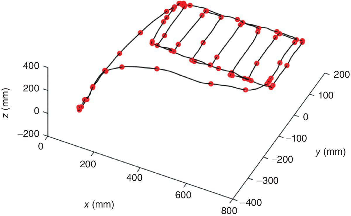
Figure 5.6 Initial assignment of key points for the trajectory with minimum distortion.
Afterward, the recorded trajectories are mapped into discrete sequences of observed symbols, and discrete HMMs are trained. For that purpose, Kevin Murphy’s HMM toolbox (Murphy, 1998) is used in MATLAB environment. The number of discrete observation symbols No is set to 256. The number of hidden states Ns is set equal to the number of key points of the minimum distortion trajectory plus 1, that is, 73. The Viterbi algorithm is employed for finding the sequences of hidden states for each observation sequence, and key points are assigned to the position and orientation values of the trajectories that correspond to the transitions between the hidden states in the observation sequences. Thus, including the starting and ending points of the trajectories, each demonstration was described by a time‐indexed sequence of 74 key points. As explained earlier, for the observation sequences with missing hidden states, the coordinates of the corresponding missing key points are set to zero (for that reason, they were referred to as null key points). This procedure results in spatiotemporal ordering of the key points for all trajectories, with a one‐to‐one mapping existing between the key points across the different demonstrations (e.g., for each trajectory, the key point with the index ![]() corresponds to the upper right corner of the contour). Log likelihoods of the observation sequences for the trained HMM are obtained with the forward algorithm. The observation sequence
corresponds to the upper right corner of the contour). Log likelihoods of the observation sequences for the trained HMM are obtained with the forward algorithm. The observation sequence ![]() had the highest log likelihood; therefore, the demonstration X3 is used for temporal alignment of the set of trajectories with the DTW algorithm.
had the highest log likelihood; therefore, the demonstration X3 is used for temporal alignment of the set of trajectories with the DTW algorithm.
To obtain a generalized trajectory that would represent the entire set, its length should be approximately equal to the average length of the trajectories in the set. Hence, the average durations of the hidden states for the trained HMM are calculated, whereby the newly created sequence of hidden states has length of 5522 time frames. This value is indeed very close to the average length of the demonstrations, being 5519. This time vector is used to modify the time flow of the demonstration X3 as explained in Section 5.2.2.3.1. Subsequently, the resulting sequence is used as a reference sequence for the DTW algorithm, that is, to align each of the demonstrated trajectories against it. The DTW alignment resulted in time‐warped trajectories with length of 5522 time frames, from which the time instances of the key points are extracted. The Cartesian positions coordinates x, y, and z of the DTW‐reassigned key points from all demonstrations are shown in Figure 5.7.

Figure 5.7 Spatiotemporally aligned key points from all demonstrations. For the parts of the demonstrations which correspond to approaching and departing of the tool with respect to the panel, the clusters of key points are more scattered, when compared to the painting part of the demonstrations.
For the approaching and departing parts of trajectories in Figure 5.7, the variance among the key points is high, which implies that these parts are not very important for reproduction. The distributions of the RMS errors for the clusters of key points along x, y, and z coordinates are shown in Figure 5.8a. There are 73 clusters of key points in total, where the starting and ending subsets of key points, which correspond to the approaching and departing parts of the trajectories, exhibit larger deviations from the centroids of the clusters. Therefore, weighting coefficients with lower values are assigned for those parts of the trajectories. The variance of the key points associated with painting the contour and the inner side of the panel is low, and thus the computed weighting coefficients have values close to 1. Values of 0.5 and 2 standard deviations of the RMS errors for the corresponding cluster are adopted for εmin and εmax, respectively, in (5.13). The weights for such adopted thresholds are displayed in Figure 5.8b. For comparison, the weighting coefficients for the key point clusters with the threshold values of 1/6 and 6 standard deviations are shown in Figure 5.8c. In this case, the weights distribution will result in a reproduction trajectory that will fit more closely the demonstrated trajectories. However, such choice of the parameters will not have very significant impact on the final outcome, that is, the approach is not highly sensitive to the choice of the threshold values εmin and εmax.

Figure 5.8 (a) RMS errors for the clusters of key points, (b) weighting coefficients with threshold values of 1/2 and 2 standard deviations, and (c) weighting coefficients with threshold values of 1/6 and 6 standard deviations.
The last step entails smoothing spline interpolation through the key points by using an empirically determined smoothing factor ![]() , which gives both satisfactory smoothness and precision in position for the considered application. For the orientation of the tool expressed in Euler roll–pitch–yaw angles, the 1D generalization results are given in Figure 5.9. The plots show the angle values of the key points and the interpolated curves for each of the angle coordinates. A plot of the Cartesian coordinates of the resulting generalized trajectory Xgen is shown in Figure 5.10.
, which gives both satisfactory smoothness and precision in position for the considered application. For the orientation of the tool expressed in Euler roll–pitch–yaw angles, the 1D generalization results are given in Figure 5.9. The plots show the angle values of the key points and the interpolated curves for each of the angle coordinates. A plot of the Cartesian coordinates of the resulting generalized trajectory Xgen is shown in Figure 5.10.

Figure 5.9 Generalization of the tool orientation from the spatiotemporally aligned key points. Roll angles are represented by a dashed line, pitch angles are represented by a solid line, and yaw angles are represented by a dash–dotted line. The dots in the plot represent the orientation angles of the key points.

Figure 5.10 Generalized trajectory for the Cartesian x–y–z position coordinates of the object.
For comparison, the distributions of velocities, accelerations, and jerks for the demonstrated trajectories by the three subjects and the generalized trajectory are shown in Figure 5.11. First, from the plot of velocity distributions, it can be concluded that the mean value of the generalized trajectory is approximately equal to the average value of the velocities from the demonstrations by all subjects. This is the result of the generalization procedure, that is, the demonstrations by all subjects are used to find a generalized trajectory that will represent the entire set of demonstrations. Second, the distributions of accelerations indicate that the values of the generalized trajectory are lower than the values of the demonstrated trajectories. It is due to the fact that spline smoothing interpolation is employed for reconstruction of the generalized trajectory, which reduces the changes of velocities present in human motions. Third, the jerk distribution for the generalized trajectory is significantly condensed when compared to the demonstrated trajectories. Namely, the inconsistency of the human motions represented by high levels of jerk is filtered out by the generalization procedure, resulting in a smooth trajectory with low levels of jerk.

Figure 5.11 Distributions of (a) velocities, (b) accelerations, and (c) jerks for the demonstrated trajectories by the subjects and the generalized trajectory.
5.2.2.4.2 Experiment 2
The second experiment entails painting a panel with more complex geometry, shown in Figure 5.12a. The objective is to paint the top side of the panel, and the horizontal plane on the right‐hand side of the panel. Both areas are shown bordered with solid lines in Figure 5.12a. The three optical markers shown in the picture are used to define the reference coordinate system of the panel. The task is demonstrated five times by a single demonstrator, and all trajectories are shown superimposed in Figure 5.12b. Different from Experiment 1 where the shape of the generalized trajectory for the painting part is obvious from Figure 5.4c, in the case of Experiment 2 it is not easy to infer the shape of the generalized trajectory, especially for the small right‐hand plane where the waving motions are not controlled.

Figure 5.12 (a) The part used for Experiment 2, with the surfaces to be painted bordered with solid lines and (b) the set of demonstrated trajectories.
The lengths of the demonstrations range between 4028 and 4266 measurements. The initial selection of candidate key points with the number of clusters ρ set to 64 results in numbers of key points between 122 and 134 per trajectory. Based on the sequence with minimum distortion, the number of hidden states Ns for training the HMM is set to 123. Afterward, the demonstrations are temporally aligned with DTW, with the length of the sequence of average states duration equal to 4141 time frames. The resulting set of key points from all five demonstrations is interpolated to generate a generalized trajectory Xgen (Figure 5.13a). The plot also shows the approach and retreat of the painting tool with respect to the panel.

Figure 5.13 (a) Generalized trajectory for Experiment 2 and (b) execution of the trajectory by the robot learner.
The generalized trajectory for the pose of the painting tool was transferred to a desktop robot (Motoman® UPJ), and afterward it was executed by the robot (Figure 5.13b). The height of the robot’s end‐effector was set up to 30 millimeters above the part. The objective of the experiments was not to perform the actual painting with the robot, but to illustrate the approach for learning complex trajectories from observations of demonstrated tasks. The results demonstrate that with encoding of demonstrations at the trajectory level, complex demonstrated movements can be modeled and generalized for reproduction by a robot in a PbD environment.
5.2.2.5 Comparison with Related Work
To compare the presented method with the similar works in the literature, the obtained trajectory for task reproduction based on the approach reported by Calinon and Billard (2004) is shown in Figure 5.14. The demonstration set for Experiment 1 from the Section 5.2.2.4.1 is used, and the result is obtained by using the same parameter values reported in the aforementioned section. The initial key points selection based on LBG algorithm is employed, in order to compare the approaches on the most similar basis. The trajectory for task reproduction is generated by smoothing spline interpolation of the key points generated from the Viterbi path of the most consistent trajectory, as explained in the work of Calinon and Billard (2004). The most consistent trajectory is shown with the dashed line in Figure 5.14. The main drawback of this approach is that it does not generalize from the demonstrated set. Instead, the reproduction trajectory is obtained by using a criterion for selecting the best demonstration from the recorded set, followed by a smoothing procedure. On the other hand, in the approach presented in the book the trajectory for the task reproduction (shown in Figure 5.10) is obtained by taking into account important features from the entire set of demonstrated trajectories, and it does not rely so heavily on only one of the demonstrated trajectories.

Figure 5.14 Generated trajectory for reproduction of the task of panel painting for Experiment 1, based on Calinon and Billard (2004). The most consistent trajectory (dashed line) corresponds to the observation sequence with the highest likelihood of being generated by the learned HMM.
Another advantage of the presented approach with respect to the work by Calinon and Billard (2004) is in providing a mechanism for interpretation of the intent of the demonstrator. Based on the variance of the key points corresponding to the same spatial features across the demonstrated set, the method presented here assigns different weights for reproduction purposes. For instance, for the approaching and departing (transitional) sections of the trajectories, the variability across the demonstrated set is high, and subsequently the generalized trajectory does not follow strictly the trajectories key points. On the other hand, the section of the trajectories corresponding to painting the panel is more constrained, which is reflected in the generation of the generalized trajectory with tight interpolation of the identified key points. It can be observed in Figure 5.10 that the approaching and departing sections are smoother, due to the higher variance across the demonstrations, whereas in Figure 5.14 the approaching and departing sections simply follow the most consistent trajectory. The procedure adopted in the book has similarities to the work of Calinon (2009) based on GMM/GMR, where the sections of the demonstration with high values of the Gaussian covariances are considered less important for reproduction purposes, and vice versa.
The approach of Asfour et al. (2006), which employs generalization from the set of demonstrations by using the concept of common key points, is similar to the presented approach, although it may provide suboptimal results in some cases. For instance, if a key point is missing in one of the demonstrated trajectories, and it is present in all of the remaining trajectories, this key point will be eliminated as not being common and will not be considered for generalization purposes. To avoid this case, the approach might require applying a heuristic for analysis of the demonstrations, and elimination of the suboptimal demonstrations.
The results from the developed method and the methods reported in Calinon and Billard (2004) and Asfour et al. (2006) are compared by using the RMS error as a metric for evaluation of learned trajectories (Calinon et al., 2010)
where m1 and m2 are used for indexing the trajectories. The trajectories were scaled to sequences with the same length by using two techniques: linear scaling and DTW alignment. With the linear scaling technique, the length is set equal to the average length of the demonstrated trajectories. For the DTW scaling, the entire set of trajectories is aligned against one of the demonstrated trajectories. Rather than selecting the generalized trajectory for scaling the dataset with the DTW, some of the demonstrated trajectories were used as reference sequences for alignment, to avoid biased results for the RMS differences.
A color map chart with the RMS differences for the linearly scaled trajectories for Experiment 1 is shown in Figure 5.15. The first three trajectories in the chart represent the generalized trajectories obtained by the presented approach—XG1, by the approach proposed in Calinon and Billard (2004)—XG2, and the one proposed in Asfour et al. (2006)—XG3. The rest of the cells correspond to the demonstrated trajectories X1–X12. The darker colors in the chart pertain to cells with smaller RMS differences. For instance, the trajectory X5 is the most dissimilar to the whole set, and it can be noted that the trajectories demonstrated by the same subject X1–X4, X5–X8, and X9–X12 are more similar when compared to the trajectories demonstrated by the other subjects.

Figure 5.15 RMS differences for the reproduction trajectories generated by the presented approach (XG1), the approaches proposed in Calinon and Billard (2004) (XG2), Asfour et al. (2006) (XG3), and the demonstrated trajectories (X1–X12). As the color bar on the right side indicates, lighter nuances of the cells depict greater RMS differences.
The sums of the RMS differences for the trajectories from Figure 5.15 are given in Figure 5.16a. The RMS differences for scaling of the trajectories with DTW are also displayed. The demonstrated trajectories X4, X5, and X12 are chosen as reference sequences for aligning the trajectories. The DTW algorithm is repeated for three of the demonstrated trajectories to avoid any subjective results that can arise from using a particular trajectory as a reference sequence. As expected, the DTW algorithm aligns the trajectories better than the linear scaling technique. For the presented four cases, the cumulative RMS differences for the trajectory obtained by the presented approach (XG1) are the smallest, which infers that it represents the best match for the demonstrated set.

Figure 5.16 Cumulative sums of the RMS differences for the reproduction trajectories generated by the presented approach (XG1), the approaches proposed in Calinon and Billard (2004) (XG2), and Asfour et al. (2006) (XG3). (a) Demonstrated trajectories (X1–X12) from Experiment 1 and (b) demonstrated trajectories (X1–X5) from Experiment 2.
Similarly, for Experiment 2 from the Section 5.2.2.4.2, the sums of the RMS differences are presented in Figure 5.16b. The DTW alignment is repeated for two of the demonstrated trajectories, X2 and X4. Based on the presented results, it can be concluded that the generalized trajectory generated by the described approach fits better the demonstrated set, when compared to the similar approaches proposed by Calinon and Billard (2004) and Asfour et al. (2006).
Another work in the literature that has some similarities to the one presented in the book has been reported by Gribovskaya and Billard (2008). In their study, DTW was employed initially to align the recorded sequences. Afterward, a continuous HMM was employed for encoding the trajectories. One drawback of such procedure is that the DTW algorithm distorts the trajectories. As a result, important spatial information from the demonstrations may be lost. In addition, the velocity profile of the DTW aligned demonstrations is deformed. In the method presented here, HMM is used for segmentation of the trajectories as recorded, and DTW is used before the interpolation procedure, only to shift the key points to a trajectory with a given time duration (which is found as the average of time durations of the hidden states form HMM). Hence, the velocity information is preserved for modeling the demonstrations with HMM, and the DTW affects the trajectories only at the level of key points.
The computational expense of the presented approach is compared with the state‐of‐the‐art approach reported in Calinon (2009), which uses GMM and GMR for modeling and generalization of continuous movements in a robot PbD setting. The simulations are run on a 2.1 GHz dual‐core CPU with 4 GB of RAM running under Windows XP in the MATLAB environment. Since there are slight variations for the processing times in different simulation trials, the codes were run five times, and the mean values and standard variations are reported. The computation times for obtaining a generalized trajectory from the sets of measured trajectories for both experiments from Section 5.2.2.4 are presented in Table 5.2. The DTW alignment step of the method is performed with a MATLAB executable (MEX) file, which increases the computational speed of the DTW algorithm for about 6–8 times compared to the standard MATLAB m‐files. The results of the computational cost for the presented approach displayed in Table 5.2 indicate that most of the processing time is spent on the learning of HMM parameters and on the discretization of the continuous trajectories.
Table 5.2 Mean values and standard deviations of the computation times for learning the trajectories from Experiment 1 and Experiment 2.
| CPU times (seconds) | ||
| Steps of the program code: | Experiment 1 | Experiment 2 |
| 1. Initial preprocessing (smoothing, removing NANs) | 0.62 (±0.27) | 0.27 (±0.01) |
| 2. LBG clustering | 38.38 (±23.20) | 5.69 (±0.50) |
| 3. HMM initialization | 185.17 (±27.05) | 51.33 (±16.76) |
| 4. HMM training | 108.41 (±22.36) | 149.43 (±36.01) |
| 5. HMM inference | 24.40 (±0.81) | 12.74 (±0.72) |
| 6. DTW alignment | 44.50 (±0.35) | 23.92 (±0.37) |
| 7. Key point weighting and interpolation | 2.56 (±1.04) | 2.28 (±0.01) |
| Total | 404.05 (±26.81) | 245.73 (±39.21) |
The computation times for the GMM/GMR method are reported in Table 5.3, with using the same MATLAB MEX subroutine for performing the DTW alignment phase. For Experiment 1, the trajectory X12 (with the length of 4939 measurements) is selected as a reference sequence for aligning the set of 12 demonstrated trajectories, whereas for Experiment 2 the trajectory X2 (4048 measurements) is selected as a reference sequence for aligning the set of five trajectories. For the steps of GMM encoding and GMR generalization, the MATLAB codes provided in Calinon (2009) are used. The number of Gaussian components for modeling the trajectories was approximated by trial and error, and the values used for the reported times are 40 for the first experiment and 75 for the second experiment.
Table 5.3 Mean values and standard deviations of the computation times for learning the trajectories from Experiment 1 and Experiment 2 by applying the GMM/GMR approach.
| CPU times (seconds) | ||
| Steps of the program code: | First experiment | Second experiment |
| 1. Initial preprocessing | 0.49 (±0.01) | 0.21 (±0.01) |
| 2. DTW alignment | 40.16 (±0.11) | 20.03 (±0.38) |
| 3. GMM encoding | 847.77 (±140.27) | 948.60 (±197.95) |
| 4. GMR | 0.70 (±0.10) | 1.22 (±0.02) |
| Total | 889.13 (±140.17) | 953.86 (±197.88) |
The generalized trajectories generated from the GMM/GMR method are given in Figure 5.17. Based on the results from Table 5.3, it can be concluded that the computational cost of modeling the 6D input data into a large number of Gaussians is computationally expensive. The total computation times with the presented approach are less than the times obtained with the GMM/GMR approach for both sets of trajectories.

Figure 5.17 Generalized trajectory obtained by the GMM/GMR method (Calinon, 2009) for (a) Experiment 1 and (b) Experiment 2, in Section 4.4.4.
5.2.3 CRF Modeling and Generalization
5.2.3.1 Related Work
One of the application domains where CRFs have been most extensively utilized is the language processing. Examples include part‐of‐speech tagging (Lafferty et al., 2001; Sutton and McCallum, 2006), shallow parsing (Sha and Pereira, 2003), and named‐entity recognition (McDonald and Pereira, 2005; Klinger et al., 2007). CRFs were reported to outperform HMMs for classification tasks in these studies. Other areas of implementation include image segmentation (He et al., 2004; Quattoni et al., 2005), gene prediction (DeCaprio et al., 2007), activity recognition (Sminchisescu et al., 2005; Vail et al., 2007a), generation of objects’ trajectories from video sequences (Ross et al., 2006), etc.
In the robot PbD environment, Kjellstrom et al. (2008) presented an approach for grasp recognition from images using CRF. Martinez and Kragic (2008) employed the support vector machine (SVM) algorithm for activity recognition in robot PbD by modeling the demonstrated tasks at a symbolic level, followed by using CRF for temporal classification of each subtask into one of the several predefined action primitives classes. The comparison results of recognition rates between HMM and CRF indicated similar performance of both methods for short actions, and higher recognition rates by CRF for the case of prolonged continuous actions.
CRF has not been implemented before for acquisition of skills at the trajectory level in the area of robot PbD. Therefore, Section 5.2.3.2 presents one such approach (Vakanski et al., 2010). Similarly to the approach presented in Section 5.2.2 that employed HMM for encoding trajectories, the hidden states of the demonstrator’s intention in executing a task are related to the trajectory key points in the observed sequences. CRF is employed for conditional modeling of the sequences of hidden states based on the evidence from observed demonstrations. A generalized trajectory for reproducing the required skill by the robot is generated by cubic spline interpolation among the identified key points from the entire set of demonstrated trajectories.
5.2.3.2 Feature Functions Formation
The developed framework for robot learning from multiple demonstrations employs the optical motion capture device Optotrak Certus® (NDI, Waterloo, Canada) for the task perception (Section 2.1). Hence, the observation sequences are associated with the continuous trajectories captured during the demonstration phase. This section discusses the formation of the feature functions ![]() in a linear chain CRF structure (Section 4.3.1), for the case when the observation sequences are human demonstrated trajectories. In general, CRFs can handle observed features of either continuous or discrete nature, whereas the hidden state variables are always of discrete nature. Structuring of the feature functions for both continuous and discrete observations is discussed next.
in a linear chain CRF structure (Section 4.3.1), for the case when the observation sequences are human demonstrated trajectories. In general, CRFs can handle observed features of either continuous or discrete nature, whereas the hidden state variables are always of discrete nature. Structuring of the feature functions for both continuous and discrete observations is discussed next.
A CRF model designed for classification of human activities from continuous trajectories as observation data is presented in the work of Vail et al. (2007b). The authors introduced the following continuous‐state feature functions:
for ![]() , where Ns denotes the number of hidden states, and d is used for indexing the dimensionality of the observed Cartesian positions ok. The notation
, where Ns denotes the number of hidden states, and d is used for indexing the dimensionality of the observed Cartesian positions ok. The notation ![]() pertains to a binary indicator function, which equals to 1 when the state at time tk is i, and 0 otherwise. To enhance the classification rate of the CRF in the article of Vail et al. (2007b), additional continuous‐state feature functions are added to the model, corresponding to the observed velocities, squared positions, etc.
pertains to a binary indicator function, which equals to 1 when the state at time tk is i, and 0 otherwise. To enhance the classification rate of the CRF in the article of Vail et al. (2007b), additional continuous‐state feature functions are added to the model, corresponding to the observed velocities, squared positions, etc.
The transition feature functions for encoding the transition scores from state i at time ![]() to state j at time tk are defined as follows:
to state j at time tk are defined as follows:
for ![]() .
.
An important remark reported in the article (Vail et al., 2007b) is that the empirical sum of the features in the log‐likelihood function (4.23) can be poorly scaled when continuous features functions are used. This can cause slow convergence of the optimization algorithms, or in the worst case, the algorithm would not converge. As a remedy, the authors proposed to perform normalization of the continuous observations to sequences with zero mean and unity variance, which improved the classification results.
Nevertheless, most of CRF’s applications in the literature deal with categorical input features (e.g., labeling words in a text), rather than continuous measurements. In that case, the observed features are mapped to a finite set of discrete symbols ![]() . The state feature functions are defined as binary indicators functions for each state‐observation pairs as follows:
. The state feature functions are defined as binary indicators functions for each state‐observation pairs as follows:
for ![]() and
and ![]() .
.
The transition feature functions ![]() are defined in an identical manner as in (5.16). The structure of CRFs allows additional observed features to be easily added to the model by generalizing the feature functions. For instance, the dependence of state transitions to the observed symbol can be modeled by adding additional feature functions
are defined in an identical manner as in (5.16). The structure of CRFs allows additional observed features to be easily added to the model by generalizing the feature functions. For instance, the dependence of state transitions to the observed symbol can be modeled by adding additional feature functions ![]() .
.
5.2.3.3 Trajectories Encoding and Generalization
The implementation of CRF in this work is based on discrete observation features, due to the aforementioned scalability problems with the continuous features. For that purpose, the continuous trajectories from the demonstrations are mapped to a discrete set of symbols by using the LBG algorithm, as described in Section 5.2.1. The output of the LBG clustering procedure is a set of discrete sequences ![]() .
.
Training the CRF model requires provision of the corresponding sequences of hidden states (i.e., labels) ![]() for each observation sequence
for each observation sequence ![]() . Similar to the approach described in Section 5.2.2, the labels are assigned to the key points along the trajectories, which are characterized by significant changes in position and velocity. The initial labeling of the trajectories is performed with the LBG technique. The clustering is carried over a set of concatenated normalized positions and velocities vectors from all demonstrated trajectories, that is,
. Similar to the approach described in Section 5.2.2, the labels are assigned to the key points along the trajectories, which are characterized by significant changes in position and velocity. The initial labeling of the trajectories is performed with the LBG technique. The clustering is carried over a set of concatenated normalized positions and velocities vectors from all demonstrated trajectories, that is, ![]() for
for ![]() ,
, ![]() , and
, and ![]() . The transitions between the cluster labels are adopted as key points. The detected initial key points resulted in the labeled sequences denoted as
. The transitions between the cluster labels are adopted as key points. The detected initial key points resulted in the labeled sequences denoted as ![]() .
.
A common challenge associated with the task modeling in robot PbD is the limited number of demonstrations available for estimation of the model parameters (since it may be frustrating for a demonstrator to perform many demonstrations, and in addition, the quality of the performance can decrease due to fatigue or other factors). Therefore, to extract the maximum information from limited training data, as well as to avoid testing on the training data, the leave‐one‐out cross‐validation technique is adopted for training purposes. This technique is based on using a single observation sequence for validation, and using the remaining observation sequences for training. For instance, to label the observed sequence which corresponds to the third demonstration ![]() , a CRF model is trained on the set consisting of the observed sequences
, a CRF model is trained on the set consisting of the observed sequences ![]() , and the corresponding state sequences
, and the corresponding state sequences ![]() obtained from the initial selection of the candidate key points. The set of parameters Λ3, estimated during the training phase using (4.23) and (4.24), is afterward employed to infer the sequence of states
obtained from the initial selection of the candidate key points. The set of parameters Λ3, estimated during the training phase using (4.23) and (4.24), is afterward employed to infer the sequence of states ![]() which maximizes the conditional probability
which maximizes the conditional probability ![]() . This procedure is repeated for each observed sequence from the dataset.
. This procedure is repeated for each observed sequence from the dataset.
The inference problem of interest here consists of finding the most probable sequence of labels for an unlabeled observation sequence. The problem is typically solved either by the Viterbi method or by the method of maximal marginals (Rabiner, 1989). The maximal marginals approach is adopted in this work. This approach is further adapted for the task at hand by introducing additional constraints for the state transitions. Namely, the hidden state sequences in the presented CRF structure are defined such that they start with the state 1 and are ordered consecutively in a left‐right structure, meaning that the state 1 can either continue with a self‐transition or transition to the state 2. Furthermore, some states might not appear in all sequences, for example, a sequence can transition from the state 5 directly to the state 7, without occurrence of the state 6. By analogy with the left‐right Bakis topology in HMMs, the contributions from the potential functions which correspond to the transitions to the past states (i.e., ![]() in (4.20) for
in (4.20) for ![]() and
and ![]() ) are minimized by setting low values for the parameters
) are minimized by setting low values for the parameters ![]() . Thereby, the transitions to the previously visited states in the model are less likely to occur. Additionally, another constraint is introduced that minimizes the possibility of transitioning to distant future states, by setting low values for the parameters
. Thereby, the transitions to the previously visited states in the model are less likely to occur. Additionally, another constraint is introduced that minimizes the possibility of transitioning to distant future states, by setting low values for the parameters ![]() for
for ![]() . As a result, the potential functions corresponding to the transitions to more than two future states have approximately zero values. These constraints reflect the sequential ordering of the hidden states in the CRF model for the considered problem.
. As a result, the potential functions corresponding to the transitions to more than two future states have approximately zero values. These constraints reflect the sequential ordering of the hidden states in the CRF model for the considered problem.
The estimation of the hidden state at time tk is based on computing the maximal marginal probabilities of the graph edges, and are solved by the forward–backward algorithm
where ![]() and
and ![]() denote the forward and backward variables which are calculated in the same recursive manner as with HMMs (Section 4.2.1). The functions Ωk in (5.18) correspond to the transition feature functions in (4.20) (Sutton and McCallum, 2006), that is,
denote the forward and backward variables which are calculated in the same recursive manner as with HMMs (Section 4.2.1). The functions Ωk in (5.18) correspond to the transition feature functions in (4.20) (Sutton and McCallum, 2006), that is,

for ![]() .
.
The classification rate comparing the initial sequence of states ![]() and the sequence of states obtained by the CRF labeling
and the sequence of states obtained by the CRF labeling ![]() is used as a measure of fit for each trajectory m
is used as a measure of fit for each trajectory m

The generation of a trajectory for reproduction of the demonstrations is analogous to the generalization procedure for HMM described in Section 5.2.2.3. To recapitulate, for each sequence of hidden states, the key points are taken to be the transitions between the states. The temporal variance across the set of sequences is tackled by employing the multidimensional DTW algorithm. The trajectory Xϕ corresponding to the states sequence with the maximum classification rate ![]() in (5.20) is selected as a reference sequence, against which all the other trajectories are aligned. This process results in temporally warped key points sequences
in (5.20) is selected as a reference sequence, against which all the other trajectories are aligned. This process results in temporally warped key points sequences ![]() , where the key points’ time stamps correspond to the time vector of the reference trajectory Xϕ. Weighting coefficients are introduced based on the variance of key points across the demonstrations associated with the same time stamps, in order to account for the relative importance for interpolation. The key points from all trajectories are afterward interpolated with a smoothing cubic spline, yielding a generalized trajectory Xgen.
, where the key points’ time stamps correspond to the time vector of the reference trajectory Xϕ. Weighting coefficients are introduced based on the variance of key points across the demonstrations associated with the same time stamps, in order to account for the relative importance for interpolation. The key points from all trajectories are afterward interpolated with a smoothing cubic spline, yielding a generalized trajectory Xgen.
5.2.3.4 Experiments
The presented concept for robot PbD is assessed through simulations of two types of manufacturing processes: painting and shot peening. Perception of the demonstrated trajectories is performed with an optical tracking device. The approach is implemented in MATLAB environment by using the CRF chain toolbox (Schmidt et al., 2008).
5.2.3.4.1 Experiment 1
The experimental setup shown in Figure 5.18a is employed to simulate the trajectories of a tool for painting target objects. The painting task is demonstrated 14 times, and it consists of first painting the contour followed by painting the interior part of the panel. The demonstrations are shown in Figure 5.18c. The trajectories lengths Tm range from 1393 to 2073 time frames. For this task, the orientation of the tool is required to be normal to the panel during the painting; therefore, it is not considered as a relevant discriminative feature. For the initial selection of key points, the trajectories are automatically segmented with the LBG algorithm using 32 clusters of discrete vectors. A total of 33 transitions between the LBG’s discrete symbols appeared in all trajectories, and these are adopted as the initial key points. The first and the last measurements of each trajectory are added as key points, resulting in 35 key points per trajectory. One sample trajectory with the identified key points is shown in Figure 5.18b. The demonstrated trajectories are discretized by utilizing the vectors consisting of normalized 3D positions and velocities ![]() . With 32 symbols used per feature, the total number of observation symbols No amounted to 192.
. With 32 symbols used per feature, the total number of observation symbols No amounted to 192.

Figure 5.18 (a) Experimental setup for Experiment 1 showing the optical tracker, the tool with attached markers and the object for painting. (b) One of the demonstrated trajectories with the initially selected key points. The arrow indicates the direction of the tool’s motion. (c) Demonstrated trajectories and the generalized trajectory.
The percentage of the average classification rates of CRFs from (5.20) calculated for different observation features are given in Table 5.4. The best classification rates are obtained when both velocities and positions are used as observation features. The generalized trajectory is shown by the thick line in Figure 5.18c, superimposed with the demonstrated trajectories. Note that even if some key points were wrongfully classified by the CRF, they would not have big impact on the generalization due to the introduced weighting scheme, which assigns low weights for fitting to the key points with high variability relative to the key points from the other trajectories.
Table 5.4 Means and standard deviations of the classification rates obtained by CRF for the painting task in Experiment 1.
| Classification rates | |
| 1. Position | 81.17 (±9.20) |
| 2. Velocity | 76.86 (±3.27) |
| 3. Position and velocity | 89.11 (±3.13) |
5.2.3.4.2 Experiment 2
The second task for evaluation of the presented approach pertains to application of a shot peening procedure for surface finishing (Irish et al., 2010). Shot peening is a process of impacting material’s surface with small spherical elements called “shots.” This process produces a compressive residual stress layer on material’s surface, which increases the resistance to cracks caused by material fatigue or stress corrosion.
Demonstration of the peening task is performed seven times, with the number of measurements Tm varying between 2438 and 2655. Conversely to the painting process in Experiment 1, where the demonstrations were simulated in the university’s lab, this task’s demonstrations were captured for a process of peening in a real industrial environment. The trajectories represent waiving motions over a curved surface (Figure 5.19). Tool’s positions, velocities, and orientations are examined as observation features. The number of clusters ρ for the initial key points selection with the LBG algorithm is set to 4. This choice is appropriate for the simple waving pattern of the task. A total of 41 key points per trajectory are identified, making the number of hidden states Ns equal to 40. One sample trajectory with the initially selected key points is shown in Figure 5.19a. The discretization of the trajectories is performed with the number of pre‐specified clusters for LBG equal to 16, that is, there are 16 discrete observation symbols for each dimension of the observed sequences.

Figure 5.19 (a) Plot of a sample demonstrated trajectory for the peening task from Experiment 2 and a set of initially selected key points, and (b) generalized trajectory for the peening experiment.
The classification rates of the trajectories segmentation with CRF are given in Table 5.5. From the results provided, it can be concluded that the velocity features are the most suitable for CRF segmentation of this example. The reason behind it is that the key points corresponding to the peaks and troughs of the traversed waving motions (Figure 5.19) are associated with the minimums of the trajectories velocities, whereas the middle parts of the waving motion corresponding to the waves’ baseline are associated with the maximums velocities. Hence, these features are invariant for the entire set, and are informative for classification purposes. With regard to the tool’s orientation, only the angles around the axis normal to the surface are taken into consideration, since the orientations around the other two axes are almost constant and do not convey important information for classification purposes. The results provided in Table 5.5 indicate that the orientation information does not improve the classification rates. Moreover, the CRF classification with the orientation as the only observation feature failed. The generalized trajectory for the case of position and velocity employed as observation features is shown in Figure 5.19b. The demonstrated trajectories are not shown in Figure 5.19b, since the demonstrations are too dissimilar, and it would be impossible to differentiate the individual demonstrations in a superimposed plot.
Table 5.5 Means and standard deviations of the classification rates obtained by CRF for the peening task in Experiment 2.
| Classification rates | |
| 1. Position | 79.06 (±4.33) |
| 2. Velocity | 94.30 (±1.79) |
| 3. Position and velocity | 94.70 (±1.55) |
| 4. Position, velocity, and orientation | 93.49 (±4.37) |
5.2.3.5 Comparisons with Related Work
The presented approach is compared to HMM, due to its wide usage for labeling and analysis of sequential data. To ensure that both methods are compared on an equal basis, a discrete form of HMM is employed, where the input data are the same discrete observation sequences ![]() and the label sequences
and the label sequences ![]() , which were used in the CRF approach. The multidimensional HMM reported by Yang et al. (1994) is implemented. Different from the 1D HMM, the multidimensional HMM has one observation matrix B(d) for each dimension d of the observed data. The model is built on an assumption that each dimension of the observed sequences is independent from the other dimensions. On the other hand, the state transition matrix A has the same form as in the 1D case. The training and inference problems are solved with small modifications of the 1D HMM (see the work of Yang et al. (1994) for details). To maintain consistency with the adopted cross‐validation testing for CRF, the HMM parameters are initialized using the CRF‐labeled data for one of the trajectories (e.g.,
, which were used in the CRF approach. The multidimensional HMM reported by Yang et al. (1994) is implemented. Different from the 1D HMM, the multidimensional HMM has one observation matrix B(d) for each dimension d of the observed data. The model is built on an assumption that each dimension of the observed sequences is independent from the other dimensions. On the other hand, the state transition matrix A has the same form as in the 1D case. The training and inference problems are solved with small modifications of the 1D HMM (see the work of Yang et al. (1994) for details). To maintain consistency with the adopted cross‐validation testing for CRF, the HMM parameters are initialized using the CRF‐labeled data for one of the trajectories (e.g., ![]() and
and ![]() ), followed by the model parameters estimation with the Baum–Welch algorithm for the rest of the trajectories (e.g.,
), followed by the model parameters estimation with the Baum–Welch algorithm for the rest of the trajectories (e.g., ![]() ). The most probable sequence of hidden states for each observation trajectory and the given model are obtained by the Viterbi algorithm. This procedure is repeated for each of the observed trajectories.
). The most probable sequence of hidden states for each observation trajectory and the given model are obtained by the Viterbi algorithm. This procedure is repeated for each of the observed trajectories.
For Experiment 1 related to the painting task, the mean classification rates for the multidimensional HMM obtained from (5.20) are reported in Table 5.6. For comparison, the classification rates obtained by the CRF approach from Table 5.4 are also provided in the rightmost column. For the three cases of observation features considered, the HMM produced lower number of correct labels than the CRF. The results from statistical analysis using paired t‐tests showed statistically significant difference in the classification rates by the CRF and HMM at a 0.05 level. The following p‐values were obtained for the different observation features: position (![]() ), velocity (
), velocity (![]() ), and position/velocity (
), and position/velocity (![]() ).
).
Table 5.6 Means and standard deviations of the classification rates obtained by HMM and CRF for the painting task from Experiment 1.
| Classification rates | ||
| HMM | CRF | |
| 1. Position | 77.69 (±1.96) | 81.17 (±9.2) |
| 2. Velocity | 74.75 (±1.99) | 76.86 (±3.27) |
| 3. Position and velocity | 86.46 (±1.20) | 89.11 (±3.13) |
For the peening task in Experiment 2, the classification rates obtained from both HMM and CRF are provided in Table 5.7. For all four types of observed features reported in the table, the HMM generates higher errors in predicting the labels. The differences in the classification performance of CRF and HMM methods are found to be statistically significant at a 0.05 level. The p‐values of the performed paired t‐tests are less than 0.01 for the different observed features in Table 5.7. It can be noted that adding the tools’ orientation degrades significantly the HMM performance. When using both positions and velocities as observed features, the classification accuracy is improved, but is still lower when compared to the CRF success rates.
Table 5.7 Means and standard deviations of the classification rates obtained by HMM and CRF for the peening task from Experiment 2.
| Classification rates | ||
| HMM | CRF | |
| 1. Position | 74.99 (±3.12) | 79.06 (±4.33) |
| 2. Velocity | 80.97 (±1.79) | 94.30 (±1.79) |
| 3. Position and velocity | 89.98 (±1.81) | 94.70 (±1.55) |
| 4. Position, velocity, and orientation | 64.50 (±4.62) | 93.49 (±4.37) |
The results are consistent with the findings in other studies in the literature (Lafferty et al., 2001; Vail et al., 2007a; Martinez and Kragic, 2008), which report higher classification accuracy of CRF when compared to HMM.
5.3 Locally Weighted Regression
Local learning methods approximate the training data locally by using a set of functions, as opposed to the global regression methods which aim to calculate a single function to fit the training data at a global level. For instance, for a continuous input function y, a global regression approach calculates a continuous output function ŷ, to minimize a cost criterion,
where xi denotes the ith vector of the input data, θ is a set of parameters of the model, ![]() is the estimated function, and ℒ(f(xi, θ), yi) is a loss function.
is the estimated function, and ℒ(f(xi, θ), yi) is a loss function.
A common choice for the loss function is the least‐squares difference, that is,
In local regression, the cost function is minimized locally, that is, C(q) is a function of the input data around a query point q. Examples of local learning models are nearest neighbor, weighted average, locally weighted regression (Atkeson et al., 1997), and locally weighted projection regression (Vijayakumar and Schaal, 2000). Nearest‐neighbor approach employs a distance function to find the nearest data within the training set to a query point, whereas weighted average, as the name implies, outputs the average of the data in the vicinity of a query point weighted by the distance between the data points and the query point. Locally weighted regression fits a surface through the data points in the vicinity of the query point by using a distance weighted regression. Locally weighted projection regression utilizes linear univariate local models by projecting the input data into a local plane.
Relevance of the data in locally learning models is defined using a distance function. A commonly used distance function is the Euclidean distance, where for a multidimensional data point ![]() and a query point
and a query point ![]() , the distance is defined as
, the distance is defined as
with j used to denote the index of the components of the vectors x and q. Other distance functions that have found use in local function approximation include diagonally weighted Euclidean distance, where M is a diagonal matrix with the mj elements acting as scaling factors for the jth dimension of the input data,

Also Mahalanobis distance is employed, which is similar to the previous distance function in (5.24); only the matrix M is allowed to have any arbitrary form, and it is not constrained to being a diagonal matrix,

Another commonly used function is Minkowski distance function, where, instead of using an L2 norm, an arbitrary, weighted or unweighted, Lp norm of the distance to the query point is employed.

Weighting functions are employed to calculate the weight of the data point x, based on a used distance function. These functions provide a smooth gradual decay with the increasing distance from the query point q. In statistics, the weighting functions are called kernel functions, and correspondingly, the problem of fitting a locally weighted function is called kernel regression. The following several weighting functions have been employed:
- 1. Inverse function uses weighting based on the power of the distance to the query point, that is,
- (5.27)

- 2. Gaussian weighting function values the weights by calculating
- (5.28)

- 3. Exponential weighting function,
- (5.29)

- 4. Quadratic weighting function, given by
- (5.30)

Similarly, a number of other weighting functions have been used; some of them developed as variants of the weighting functions given in (5.27)–(5.30).
Locally weighted regression employs weighting of the input data to calculate a continuous output function ŷ,

where, as a reminder, xi denotes the ith vector in the training input data.
Another approach for performing locally weighted regression is, instead of weighting the data points, to weight the training criterion, that is, the error in fitting the function, as in
In this case, the approximation function ![]() fits local models to the data, with the model parameters θ depending of the input data in the vicinity of the query point q. Accordingly, the approximation function will produce different set of model parameters for different query points.
fits local models to the data, with the model parameters θ depending of the input data in the vicinity of the query point q. Accordingly, the approximation function will produce different set of model parameters for different query points.
Linear models for locally weighted regression utilize a set of local models that are linear in the unknown parameters θ. The weighting functions in linear local models are commonly called basis functions. In the case of linear locally weighted regression, the cost function becomes
This approach allows fast approximation of nonlinear functions, where the computational cost increases linearly with the number of inputs. These advantages render it suitable for real‐time applications.
The method of locally weighted regression has been applied in robotic learning from demonstration based on the dynamical systems approach described in Section 4.4. In this case, a set of Gaussian basis functions are employed to locally approximate a nonlinear force function F, related to a set of observed trajectories.
To learn a task from demonstrations, the nonlinear force function F is calculated from (4.26) by substituting the values for the position, velocity, and acceleration, denoted x1, ![]() , and
, and ![]() , of observed trajectories,
, of observed trajectories,
Next, the phase variable ϕ is obtained by integrating the canonical system (4.27), and the weights wi in (4.29) are calculated that minimize the cost function
by solving a linear regression problem. The weighting Gaussian functions are given in (4.30). Weighted Euclidean distance is employed as a distance function, where the standard deviation of the Gaussian basis functions is used as a weighting distance factor. Similarly, for learning motion primitives in rhythmic tasks, von Mises basis functions, given in (4.31), are adopted due to the periodic nature of the input trajectories.
To recreate a generalized trajectory that will converge toward a goal location xgoal, the weights wi obtained by solving (5.35), and corresponding to the data for observed task trajectories, are reused. The value of the canonical variable ϕ is set to 1 at the beginning of the movement, and the canonical system (4.27) is integrated at each time step to obtain the current value of the variable, thus driving the value of the function F. The method produces a smooth output trajectory that converges toward the discrete goal, with the task execution strategy being robust to perturbations to the state x.
5.4 Gaussian Process Regression
Within the published literature, a body of work employed Gaussian processes for robot leaning from human demonstrations (Shon et al., 2005; Grimes et al., 2006; Schneider and Ertel, 2010).
In general, Gaussian processes theory is used for learning the distribution of a regression function f given a set of input variables ![]() and noisy observed target variables
and noisy observed target variables ![]() . The target variables are modeled as
. The target variables are modeled as ![]() , where ε is a random noise variable that is assumed to be independent and identically distributed with respect to the observed variables. The Gaussian process regression (GPR) model calculates a predictive distribution
, where ε is a random noise variable that is assumed to be independent and identically distributed with respect to the observed variables. The Gaussian process regression (GPR) model calculates a predictive distribution ![]() , where x* denotes a new input value, and
, where x* denotes a new input value, and ![]() is a set of tuples consisting of n input points and related observations,
is a set of tuples consisting of n input points and related observations, ![]() . Gaussian processes consider the predicted values as samples from a zero‐mean Gaussian distribution, resulting in a predictive Gaussian distribution
. Gaussian processes consider the predicted values as samples from a zero‐mean Gaussian distribution, resulting in a predictive Gaussian distribution ![]() with mean (Schneider and Ertel, 2010)
with mean (Schneider and Ertel, 2010)
and covariance matrix
In these equations ![]() denotes the noise variance, whereas the covariance matrices K, K*, K** are defined by a covariance function, or kernel,
denotes the noise variance, whereas the covariance matrices K, K*, K** are defined by a covariance function, or kernel, ![]() , as
, as ![]() ,
, ![]() , and
, and ![]() .
.
A variety of kernel functions are used in the literature, with the most common being the squared exponential kernel, also known as the radial basis function kernel, given with

where ![]() denotes the signal variance and l denotes the characteristic length scale. The set of parameters
denotes the signal variance and l denotes the characteristic length scale. The set of parameters ![]() ,
, ![]() , and l are referred to as hyper parameters of the covariance function, and their selection defines the form of the kernel. A standard approach for obtaining the values of the hyper parameters is by using the conjugate gradient algorithm to maximize the log likelihood of the data with respect to the hyper parameters. If the symbol ω substitutes the hyper parameters
, and l are referred to as hyper parameters of the covariance function, and their selection defines the form of the kernel. A standard approach for obtaining the values of the hyper parameters is by using the conjugate gradient algorithm to maximize the log likelihood of the data with respect to the hyper parameters. If the symbol ω substitutes the hyper parameters ![]() , and
, and ![]() denotes the matrix of the input data, the log marginal likelihood is given by
denotes the matrix of the input data, the log marginal likelihood is given by
In (5.39), the notation ![]() refers to determinant of a matrix, and
refers to determinant of a matrix, and ![]() .
.
A shortcoming of using GPR for real‐world applications is the high computational cost of the algorithm. To reduce the computational expense, Schneider and Ertel (2010) proposed a local Gaussian process model in a PbD setting, where the prediction mean and the covariance are calculated as the Gaussian product of local model predictions,

where

and z is the normalization constant. The approximate prediction function is then used for reconstructing an execution trajectory from a set of observed trajectories.
5.5 Summary
Approaches for generating a trajectory for task reproduction by a robot learner are reviewed in this chapter. GMR method employs a mixture of Gaussian density functions to calculate the conditional expectation of the temporal component of the demonstrated trajectories given the spatial component of the trajectory. Task planning with spline regression employs a set of trajectories key points, related to the transitions between the hidden states in the statistical models of HMM and CRF. Locally weighted regression is used for trajectory generation with tasks encoded via DMPs. GPR has also been employed for modeling a set of hidden and observed states from demonstration, followed by creating a task reproduction trajectory.
The chapter describes the entire procedure of transferring skills to robots for two industrial tasks: painting and shot peening. HMM and CRF are used for encoding of demonstrated tasks as a set of relevant key points, whereas DTW is employed for temporal clustering of the key points into a format that represents the generalized time flow of all demonstrations. A generalized trajectory for task reproduction is produced by interpolation of the key points across the demonstrated trajectories using spline regression.
References
- Akaike, H., (1974). A new look at the statistical model identification. IEEE Transactions on Automatic Control, vol. 19, no. 6, pp. 716–723.
- Aleotti, J., and Caselli, S., (2006). Robust trajectory learning and approximation for robot programming by demonstration. Robotics and Autonomous Systems, vol. 54, no. 5, pp. 409–413.
- Asfour, T., Gyarfas, F., Azad, P., and Dillmann, R., (2006). Imitation learning of dual‐arm manipulation tasks in a humanoid robot. Proceedings of the International Conference on Humanoid Robots, Genoa, Italy, pp. 40–47.
- Atkeson, C.G., Moore, A.W., and Schaal, S., (1997). Locally weighted learning for control. Artificial Intelligence Review, vol. 11, no. 1–5, pp. 75–113.
- Berkhin, P., (2001). Survey of clustering data mining techniques. Grouping Multidimensional Data, Springer, pp. 25–71.
- Bezdek, D., (1981). Pattern Recognition with Fuzzy Objective Function Algorithms. New York, USA: Plenum Press.
- Billard, A., Eppars, Y., Calinon, S., Schaal, S., and Cheng, G., (2004). Discovering optimal imitation strategies. Robotics and Autonomous Systems, vol. 47, no. 2–3, pp. 69–77.
- Calinon, S., (2009). Robot Programming by Demonstration: A Probabilistic Approach. Boca Raton, USA: EPFL/CRC Press.
- Calinon, S., and Billard, A., (2004). Stochastic gesture production and recognition model for a humanoid robot. Proceedings of IEEE/RSJ International Conference on Intelligent Robots and Systems, Sendai, Japan, pp. 2769–2774.
- Calinon, S., and Billard, A., (2007). Learning of gestures by imitation in a humanoid robot. Imitation and Social Learning in Robots, Humans and Animals: Social and Communicative Dimension. (Eds.) Dautenhahn, K., and Nehaniv, C.L., Cambridge, USA: Cambridge University Press, pp. 153–178.
- Calinon, S., D’halluin, F., Sauser, E.L., Caldwell, D.G., and Billard, A.G., (2010). Learning and reproduction of gestures by imitation: an approach based on hidden Markov model and Gaussian mixture regression. IEEE Robotics and Automation Magazine, vol. 17, no. 2, pp. 44–54.
- Davies, D.L., and Bouldin, D.W., (1979). A cluster separation measure. IEEE Transactions on Pattern Analysis and Machine Intelligence, vol. 1, no. 2, 224–227.
- DeCaprio, D., Vinson, J.P., Pearson, M.D., Montgomery, P., Doherty, M., and Galagan, J.E., (2007). Conrad: Gene prediction using conditional random fields, Genome Research, vol. 17, no. 9, pp. 1389–1396.
- Gribovskaya, E., and Billard, A., (2008). Combining dynamical systems control and programming by demonstration for teaching discrete bimanual coordination tasks to a humanoid robot. Proceedings of ACME/IEEE International Conference on Human‐Robot Interaction, Amsterdam, the Netherlands, pp. 1–8.
- Grimes, D.B., Chalodhorn, R., and Rao, R.P.N., (2006). Dynamic imitation in a humanoid robot through nonparameteric probabilistic inference. Proceedings of Robotics: Science and Systems, Cambridge, USA: MIT Press.
- He, X., Zemel, R.S., and Carreira‐Perpinan, M.A., (2004). Multiscale conditional random fields for image labeling. Proceedings of IEEE Computer Society Conference on Computer Vision and Pattern Recognition, Washington, USA, pp. 695–702.
- Inamura, T., Tanie, H., and Nakamura, Y., (2003). Keyframe compression and decompression for time series data based on the continuous hidden Markov model. Proceedings of IEEE/RSJ International Conference on Intelligent Robots and Systems, Las Vegas, USA, pp. 1487–1492.
- Inamura, T., Kojo, N., and Inaba, M., (2006). Situation recognition and behavior induction based on geometric symbol representation of multimodal sensorimotor patterns. Proceedings of IEEE/RSJ International Conference on Intelligent Robots and Systems, Beijing, China, pp. 5147–5152.
- Irish, A., Mantegh, I., and Janabi‐Sharifi, F., (2010). A PbD approach for learning pseudo‐periodic robot trajectories over curved surfaces. Proceedings of IEEE/ASME International Conference on Advanced Intelligent Mechatronics, Montréal, Canada, pp. 1425–1432.
- Kass, R.E., and Raftery, A.E., (1995). Bayes factors. Journal of the American Statistical Association, vol. 90, no. 430, pp. 773–795.
- Kaufman, L., and Rousseeuw, P., (1990). Finding Groups in Data: An Introduction to Cluster Analysis. New York, USA: John Wiley & Sons, Inc.
- Kjellstrom, H., Romero, J., Martinez, D., and Kragic, D., (2008). Simultaneous visual recognition of manipulation actions and manipulated objects. Proceedings of European Conference on Computer Vision, Part II, LNCS 5303, pp. 336–349.
- Klinger, R., Furlong, L.I., Friedrich, C.M., Mevissen, H.T., Fluck, J., Sanz, F., et al., (2007). Identifying gene specific variations in biomedical text. Journal of Bioinformatics and Computational Biology, vol. 5, no. 6, pp. 1277–1296.
- Lafferty, J., McCallum, A., and Pereira, F., (2001). Conditional random fields: probabilistic models for segmenting and labeling sequence data. Proceedings of International Conference on Machine Learning, Williamstown, USA, pp. 282–289.
- Lee, H.‐K., and Kim, J.H., (1999). An HMM‐based threshold model approach for gesture recognition. IEEE Transactions on Pattern Analysis and Machine Intelligence, vol. 21, no. 10, pp. 961–973.
- Lee, D., and Nakamura, Y., (2006). Stochastic model of imitating a new observed motion based on the acquired motion primitives. Proceedings of IEEE/RSJ International Conference on Intelligent Robots and Systems, Beijing, China, pp. 4994–5000.
- Linde, Y., Buzo, A., and Gray, R.M., (1980). An algorithm for vector quantizer design. IEEE Transactions on Communications, vol. 28, no. 1, pp. 84–95.
- Liu, G., Zhang, J., Wang, W., and McMilan, L., (2005). A system for analyzing and indexing human‐motion databases. Proceedings of International Conference on Management of Data, Baltimore, USA, pp. 924–926.
- Martinez, D., and Kragic, D., (2008). Modeling and recognition of actions through motor primitives. Proceedings of IEEE International Conference on Robotics and Automation, Pasadena, USA, pp. 1704–1709.
- McDonald, R., and Pereira, F., (2005). Identifying gene and protein mentions in text using conditional random fields. BMC Bioinformatics, vol. 6, no. S6, pp. 1–3.
- Murphy, K., (1998). Hidden Markov Model (HMM) Toolbox for MATLAB. Available from: http://www.cs.ubc.ca/~murphyk/Software/HMM/hmm.html (accessed on September 14, 2016).
- Pook, P.K., and Ballard, D.H., (1993). Recognizing teleoperated manipulations. Proceedings of IEEE International Conference on Robotics and Automation, Atlanta, USA, pp. 578–585.
- Quattoni, A., Collins, M., and Darrell, T., (2005). Conditional random fields for object recognition. Advances in Neural Information Processing Systems, Cambridge, USA: MIT Press, pp. 1097–1104.
- Rabiner, L., (1989). A tutorial on hidden Markov models and selected applications in speech recognition. Proceedings of the IEEE, vol. 77, no. 2, pp. 257–286.
- Rice, J., and Rosenblatt, M., (1983). Smoothing splines: regression, derivatives and deconvolution. The Annals of Statistics, vol. 11, no. 1, pp. 141–156.
- Rissanen, J., (1978). Modeling by shortest data description. Automatica, vol. 14, no. 5, pp. 465–658.
- Ross, D.A., Osindero, S., and Zemel, R.S., (2006). Combining discriminative features to infer complex trajectories. Proceedings of International Conference on Machine Learning, Pittsburgh, USA, pp. 761–768.
- Schmidt, M., Swersky, K., and Murphy, K., (2008). Conditional Random Field Toolbox for MATLAB. Available from: http://www.cs.ubc.ca/~murphyk/Software/CRF/crf.html (accessed on September 14, 2016)
- Schneider, M., and Ertel, W., (2010). Robot learning by demonstration with local Gaussian process regression. Proceedings of IEEE/RAS International Conference on Intelligent Robots and Systems, Taipei, Taiwan, pp. 255–260.
- Schwarz, G., (1978). Estimating the dimension of a model. Annals of Statistics, vol. 6, no. 2, pp. 461–464.
- Sha, F., and Pereira, F., (2003). Shallow parsing with conditional random fields. Proceedings of Conference of the North American Chapter of the Association for Computational Linguistics on Human Language Technology, Stroudsburg, USA, pp. 213–220.
- Shon, A.P., Grochow, K., and Rao, R.P.N., (2005). Robotic imitation from human motion capture using Gaussian processes. Proceedings of Fifth IEEE‐RAS International Conference on Humanoid Robots, Tsukuba, Japan, pp. 129–134.
- Sminchisescu, C., Kanaujia, A., Li, Z., and Metaxas, D., (2005). Conditional models for contextual human motion recognition. Proceedings of IEEE International Conference on Computer Vision, Beijing, China, pp. 1808–1815.
- Smyth, P., (1998). Model selection for probabilistic clustering using cross‐validated likelihood, UCI‐ICS Technical Report 98‐09, University of California, Irvine, USA.
- Sutton, C., and McCallum, A., (2006). An Introduction to Conditional Random Fields for Relational Learning. (Eds.) Getoor, L., and Taskar, B., Cambridge, USA: MIT Press.
- Tso, S.K., and Liu, K.P., (1997). Demonstrated trajectory selection by hidden Markov model. Proceedings of International Conference on Robotics and Automation, Albuquerque, USA, pp. 2713–2718.
- Vail, D.L., Lafferty, J.D., and Veloso, M.M., (2007a). Feature selection in conditional random fields for activity recognition. Proceedings of IEEE/RSJ International Conference on Intelligent Robots and Systems, San Diego, USA, pp. 3379–3384.
- Vail, D.L., Veloso, M.M., and Lafferty, J.D., (2007b). Conditional random fields for activity recognition. Proceedings of International Conference on Autonomous Agents and Multi‐agent Systems, Honolulu, USA, pp. 235–243.
- Vakanski, A., Janabi‐Sharifi, F., Mantegh, I., and Irish, A., (2010). Trajectory learning based on conditional random fields for robot programming by demonstration. Proceedings of IASTED International Conference on Robotics and Applications, Cambridge, USA, pp. 401–408.
- Vakanski, A., Mantegh, I., Irish, A., and Janabi‐Sharifi, F., (2012). Trajectory learning for robot programming by demonstration using hidden Markov model and dynamic time warping. IEEE Transactions on Systems, Man, and Cybernetics—Part B: Cybernetics, vol. 44, no. 4, pp. 1039–1052.
- Vijayakumar, S., and Schaal, S., (2000). Locally weighted projection regression: an O(n) algorithm for incremental real time learning in high dimensional space. Proceedings of International Conference on Machine Learning, San Francisco, USA, pp. 1079–1086.
- Yang, J., Xu, Y., and Chen, C.S., (1994). Hidden Markov model approach to skill learning and its application to telerobotics. IEEE Transactions on Robotics and Automation, vol. 10, no. 5, pp. 621–631.
- Yang, J., Xu, Y., and Chen, C.S., (1997). Human action learning via hidden Markov model. IEEE Transactions on Systems, Man, and Cybernetics—Part A, vol. 27, no. 1, pp. 34–44.
- Zhou, F., De la Torre, F., and Hodgins, J.K., (2008). Aligned cluster analysis for temporal segmentation of human motion. Proceedings of IEEE Conference on Automatic Face and Gestures Recognition, Amsterdam, the Netherlands, pp. 1–7.