
6
Task Execution
This chapter focuses on endowing robustness in the task execution step using vision‐based robot control. A framework that performs all the steps of the learning process in the image space of a vision sensor is presented. The steps of task perception, task planning, and task execution are formulated with the goal of improved overall system performance and enhanced robustness to modeling and measurement errors. The constraints related to vision‐based controller are incorporated into the trajectory learning process, to guarantee feasibility of the generated plan for task execution. Hence, the task planning is solved as a constrained optimization problem, with an objective to optimize a set of trajectories of scene features in the image space of a vision camera.
6.1 Background and Related Work
The developed approach for robot programming by demonstration (PbD) is based on the following postulations: (i) perception of the demonstrations is performed with vision cameras; and (ii) execution of the learned strategies is conducted using visual feedback from the scene.
The most often used perception sensors in the PbD systems are the electromagnetic (Dillmann, 2004), inertial (Calinon, 2009) and optical marker‐based sensors (Vakanski et al., 2010). However, attaching sensors on workpieces, tools, or other objects for demonstration purposes is impractical, tiresome, and for some tasks, impossible. This work concentrates on using vision sensors for perception of demonstrated actions in a PbD framework, due to the nonintrusive character of the measurements. Also, visual perception is the most acceptable sensing modality for the next generation of intelligent robots, through the usage of “robots’ eyes” (probably in combination with the information gathered by other cameras or sensors located on robot’s structure).
Another important aspect of the PbD process that has received little attention is the step of task execution, being often considered as an independent step from the task planning, for which it is assumed that different types of robot control techniques can be employed. In practice, however, the type of controller used for reproduction of a planned strategy can impose certain constraints on the system, which might render the robot performance unsuitable for achieving the task goals. For example, the required command velocities and/or accelerations might not be realizable by the robot learner, or the required motions might violate the robot’s dexterous workspace limits. Therefore, in this work, both the task planning and the task execution (control) are considered synergistically.
From the control perspective, the uncertainties in the execution step can cause incorrect positioning of the robot’s end point with respect to the scene objects. For instance, joints’ gear backlashes or slippages, bending of the robot links, poor fixturing of the objects, or incorrect estimation of the poses of scene objects from noisy sensor measurements, can all have unfavorable effects on system’s performance. Under these circumstances, the execution of the generated PbD strategy from the planning phase will rely on open‐loop kinematic chain to position the end‐effector, and hence it can fail to correctly reproduce the desired robot configurations. To address the robustness of robots’ positioning under uncertainties during the task execution, a vision‐based control strategy (i.e., visual servoing) is employed here (Hutchinson et al., 1996; Janabi‐Sharifi, 2002; Chaumette and Hutchinson, 2006). At present, the use of visual feedback information in the PbD literature is mainly limited to look‐and‐move control, meaning that vision cameras are only used for extracting the positions and/or orientations of objects in the scene, without being used directly for real‐time control of robots’ motion.
The approach presented employs a set of demonstrations captured as trajectories of relevant scene features projected onto the image plane of a stationary camera. A Kalman smoother (Rauch et al., 1965) is initially employed to extract a generalized trajectory for each image feature. This set of trajectories represents smooth and continuous averages of the observed feature trajectories, and it is going to be used as reference trajectories in generating a plan for task reproduction. Similarly, a Kalman smoother is employed for obtaining reference velocities of the tracked object from the demonstrations. The planning step is formulated as an optimization problem, with a cost function that minimizes the distances between the current and reference image feature vectors and the current and reference object velocities. The constraints in the optimization model include visual, workspace, and robot constraints. All the constraints are formulated in a linear or conic form, thus enabling to solve the model as a convex optimization problem. The main advantage of employing convex optimization is the global convergence within the set of feasible solutions. Subsequently, an image‐based visual servoing (IBVS) controller is employed to ensure robust execution of the generated feature trajectories in presence of uncertainties, such as image noise and camera modeling errors (Nematollahi et al., 2012). Note that instead of Kalman smoothing, the initial generalization can be performed by other learning methods, such as the ones using hidden Markov model (HMM) or conditional random field (CRF) described in Chapter 4, or alternatively it can be performed by employing standard curve smoothing techniques. The Kalman smoothing algorithm was selected in this work as a trade‐off between the computational speed of the smoothing algorithms and the generalization abilities of the learning algorithms.
The motivations for implementing image‐based learning approach are multifold, as follows:
- Integration of a vision‐based control strategy into a PbD framework for robust task execution
- Formulation of the planning process as a convex optimization problem to incorporate important task constraints, which are often neglected in the PbD domain
- Introduction of a unique framework for PbD learning with all the steps of the PbD process, that is, observation, planning, and execution steps, taking place in the image space (of a robot’s vision system)
Only a few works in the literature deal with the problem of image‐based control in the robot learning context. Asada et al. (2000) addressed the problem of different viewpoints of demonstrated actions between a teacher and a learner agent. In this work, two pairs of stereo cameras were used separately for observation of the demonstrations and for reproduction of the planned strategies, and a PA‐10 Mitsubishi robot was employed both as a demonstrator and a learner. This approach avoids the three‐dimensional (3D) reconstruction of the observed motions, by proposing a direct reconstruction of the demonstrated trajectory in the image plane of the learner. The epipolar constraint of stereo cameras was used for this purpose, which dictates that the projections of a point onto stereo cameras lay on the epipolar lines. Visual servoing control was employed afterward for execution of the projected trajectory onto the image plane of the learner entity. Different from the approach presented in this chapter, the work by Asada et al. (2000) focuses on imitation of a single demonstrated trajectory, by tackling solely the problem of transforming a demonstrated trajectory from the demonstrated image space into the image space of the robot learner.
Jiang and Unbehauen (2002) and Jiang et al. (2007) presented iterative image‐based learning schemes, where a single static camera was used for observation of a demonstrated trajectory. The later work employed neural networks to learn an approximation of the image Jacobian matrix along the demonstrated trajectories, whereas the former work approximated directly the control signal from the demonstrated data. The learning laws were designed to reduce iteratively the tracking errors in several repetitive reproduction attempts by a robot learner, leading to convergence of the reproduced trajectory toward the demonstrated trajectory. Visual servoing control was employed for execution of the task in the image plane of the camera. Similar to the previously mentioned work in Asada et al. (2000), the proposed schemes consider imitation of a single demonstrated trajectory. Other shortcomings encompass the lack of integration of task constraints, and the possibilities of features leaving the field of view (FoV) of the camera, especially during the first or second repetitive trials when the tracking errors can be significant.
A similar work that also implements learning of the image Jacobian matrix was proposed by Shademan et al. (2009). Image‐based control was employed for execution of several primitive skills, which entailed pointing and reaching tasks. Numerical estimation of the Jacobian matrix was established via locally least‐square estimation scheme. However, this approach is limited to the learning of only several primitive motions, without providing directions of how it can be implemented for learning complex trajectories from demonstrations.
On the other hand, a large body of work in the literature is devoted to the path planning in visual servoing (Mezouar and Chaumette, 2002; Deng et al., 2005; Chesi and Hung, 2007). The majority of these methods utilize an initial and a desired image of the scene, and devise a plan for the paths of salient image features in order to satisfy certain task constraints. Different from these works, the planning step in the framework presented here is initialized by multiple examples of the entire image feature trajectories that are acquired from the demonstrations. Additionally, the planning in this work is carried out directly in the image plane of a vision sensor. However, since direct planning in the image space can cause suboptimal trajectories of the robot’s end point in the Cartesian space, a constraint is formulated in the model that forces the respective Cartesian trajectory to stay within the envelope of the demonstrated motions.
6.2 Kinematic Robot Control
Robot control involves establishing the relationship between the joint angles and the position and orientation (pose) of the robot’s end point. From this aspect, for a given vector of robot joint angles ![]() , the forward robot kinematics calculates the pose of the end‐effector (Sciavicco and Siciliano, 2005). Denavit−Hartenberg convention is a common technique for assigning coordinate frames to a robot’s links, as well as for calculating the forward kinematics as a product of homogenous transformation matrices related to the coordinate transformation between the robot links frames
, the forward robot kinematics calculates the pose of the end‐effector (Sciavicco and Siciliano, 2005). Denavit−Hartenberg convention is a common technique for assigning coordinate frames to a robot’s links, as well as for calculating the forward kinematics as a product of homogenous transformation matrices related to the coordinate transformation between the robot links frames

In the given equation, ![]() and
and ![]() denote the rotation matrix and the position vector, respectively, of the end‐effector frame with respect to the robot base frame.
denote the rotation matrix and the position vector, respectively, of the end‐effector frame with respect to the robot base frame.
The reverse problem of finding the set of joint angles corresponding to a given pose of the end‐effector is called robot inverse kinematics. The equations of the inverse kinematics for a general robot type are nonlinear, and a closed‐form solution does not exist. Robot control is therefore commonly solved using robot differential kinematics equations. In particular, the relation between the joint velocities and the resulting velocities of the end‐effector is called forward differential kinematics, expressed by the following equation:
The matrix J(q) in (6.2) is called the robot Jacobian matrix, and provides a linear mapping between the joint and end‐effector velocities. The forward differential kinematics can be easily derived for a generic robot type. The derivation of the equations for calculating the Jacobian matrix can be found in any textbook that covers robot modeling (e.g., Sciavicco and Siciliano, 2005).
The inverse differential kinematics problem solves the unknown set of joint velocities corresponding to given end‐effector velocities. It is obtained by calculating the inverse of the Jacobian matrix in (6.2), that is,
under the assumption that the Jacobian matrix is square and nonsingular. Obtaining the joint angles for robot control purposes is typically based on numerical integration of (6.3) over time.
Note that the Jacobian matrix is of size ![]() ; therefore, the inverse of the Jacobian matrix will not exist for robots with number of joints different from 6. If
; therefore, the inverse of the Jacobian matrix will not exist for robots with number of joints different from 6. If ![]() , the inverse kinematics problem can be solved by using the right pseudoinverse of the Jacobian matrix,
, the inverse kinematics problem can be solved by using the right pseudoinverse of the Jacobian matrix, ![]() . In this case, the solution to (6.2) is
. In this case, the solution to (6.2) is
where ![]() is any arbitrary vector.
is any arbitrary vector.
The joint configurations for which the Jacobian matrix is singular are called robot kinematic singularities, and the corresponding configurations will be singular configurations. These configurations may lead to unstable behavior, for example, unbounded joint velocities, and should be avoided if possible.
6.3 Vision‐Based Trajectory Tracking Control
Visual servoing systems are generally categorized into three main servoing structures (Chaumette and Hutchinson, 2006): position‐based visual servoing (PBVS), image‐based visual servoing (IBVS), and hybrid visual servoing (HVS). With regards to the position of the camera(s) of the visual servoing systems, there are two configurations: camera mounted on robot’s end‐effector (a.k.a. camera‐in‐hand or eye‐in‐hand), and camera in a fixed position with respect to the end‐effector (camera‐off‐hand).
6.3.1 Image‐Based Visual Servoing (IBVS)
IBVS is based on positioning of the end‐effector with respect to target objects by using feature parameters in the image space. Coordinates of several points from the target object can be considered as image feature parameters. Therefore, let the coordinates of n object feature points in the sworld frame are denoted with (Xi, Yi, Zi), for i = 1, 2, …, n. The perspective projections of the feature points in the image plane are ![]() , where
, where

Here, f denotes the focal length of the camera, u and v are pixel coordinates of the corresponding image features, u0 and v0 are pixel coordinates of the principal point, and α denotes the aspect ratio of horizontal and vertical pixel dimensions. The set of all vectors of image feature parameters ![]() defines the image space
defines the image space ![]() . Let s* denote the vector of desired image feature parameters, which is constant for the task of positioning of the robot’s end‐effector with respect to a stationary target object.
. Let s* denote the vector of desired image feature parameters, which is constant for the task of positioning of the robot’s end‐effector with respect to a stationary target object.
The goal of IBVS is to generate a control signal, such that error in the image space ![]() is minimized, subject to some constraints. For the case of an eye‐in‐hand configuration, it can be assumed that the camera frame coincides with the end‐effector frame, and the relationship between the time change of camera velocity and the image feature parameters is given with
is minimized, subject to some constraints. For the case of an eye‐in‐hand configuration, it can be assumed that the camera frame coincides with the end‐effector frame, and the relationship between the time change of camera velocity and the image feature parameters is given with
where vc denotes the spatial camera velocity in the camera frame, and the matrix L(s) is referred to as image Jacobian or interaction matrix. For a perspective projection model of the camera, the interaction matrix is given as (Chaumette and Hutchinson, 2006)

Note that Zi is the depth coordinate of the target feature i with respect to the camera frame, whose value has to be estimated or approximated for computation of the interaction matrix.
For a properly selected set of features, traditional control laws based on exponential decrease of the error in image space ensures local asymptotic stability of the system and demonstrates good performance. Compared to PBVS, IBVS is less sensitive to camera calibration errors, does not require pose estimation, and is not as computationally expensive. On the other hand, the control law with exponential error decrease forces the image feature trajectories to follow straight lines, which causes suboptimal Cartesian end‐effector trajectories (Figure 6.1). That is especially obvious for tasks with rotational camera movements, when the camera retreats along the optical axis and afterward returns to the desired location (Chaumette, 1998).


Figure 6.1 Response of classical IBVS: feature trajectories in the image plane, camera trajectory in Cartesian space, camera velocities, and feature errors in the image plane.
6.3.2 Position‐Based Visual Servoing (PBVS)
PBVS systems use information for feature parameters extracted from image space to estimate the pose of an end‐effector with respect to a target object. The control is designed based on the relative error between estimated and desired poses of the end‐effector in the Cartesian space. There are several approaches for end‐effector pose estimation in the literature, including close‐range photogrammetric techniques (Yuan, 1989), analytical methods (Horaud et al., 1989), least‐squares methods (Liu et al., 1990), and Kalman filter estimation (Wilson et al., 2000; Ficocelli and Janabi‐Sharifi, 2001).
Let ![]() denotes the translation vector of the frame attached to the camera with respect to the desired camera frame, and let use angle/axis parameterization for the orientation of the camera with respect to the desired camera frame
denotes the translation vector of the frame attached to the camera with respect to the desired camera frame, and let use angle/axis parameterization for the orientation of the camera with respect to the desired camera frame ![]() . The relative error between the pose of the current and desired pose of the camera is
. The relative error between the pose of the current and desired pose of the camera is ![]() . The relationship between the time change of the pose error and the camera velocity
. The relationship between the time change of the pose error and the camera velocity ![]() is given by the interaction matrix
is given by the interaction matrix

where I3 is a 3 × 3 identity matrix, and matrix Lθu is defined as (Malis et al., 1999)

where ![]() and
and ![]() . For the case of control with exponential decrease of the error (i.e.,
. For the case of control with exponential decrease of the error (i.e., ![]() ), the camera velocity is
), the camera velocity is

The final result in (6.10) follows from ![]() (Malis et al., 1999). The described control causes the translational movement of the camera to follow a straight line to the desired camera position, which is shown in Figure 6.2. On the other hand, the image features in Figure 6.2 followed suboptimal trajectories, and left the camera boundaries.
(Malis et al., 1999). The described control causes the translational movement of the camera to follow a straight line to the desired camera position, which is shown in Figure 6.2. On the other hand, the image features in Figure 6.2 followed suboptimal trajectories, and left the camera boundaries.


Figure 6.2 Response of classical PBVS: feature trajectories in the image plane, camera trajectory in Cartesian space, camera velocities, and feature errors in the image plane.
The advantages of PBVS stem from separation of the control design from the pose estimation, which endows the use of traditional robot control algorithms in the Cartesian space. This approach provides good control for large movements of the end‐effector. However, the pose estimation is sensitive to camera and object model errors and it is computationally expensive. In addition, it does not provide a mechanism for regulation of features in the image space, which can cause features to leave the camera FoV (Figure 6.2).
6.3.3 Advanced Visual Servoing Methods
Hybrid visual servo techniques have been proposed to alleviate the limitations of IBVS and PBVS systems. In particular, HVS methods offer a solution to the problem of camera retreat through decoupling of the rotational and translational degrees of freedom (DoFs) of the camera. The hybrid approach of 2‐1/2‐D (Malis et al., 1999) utilizes extracted partial camera displacement from the Cartesian space to control the rotational motion of the camera, and visual features from the image space to control the translational camera motions. Other HVS approaches include the partitioned method (Corke and Hutchinson, 2001), which partitions the control of the camera along the optical axis from the control of the remained DoFs, and the switching methods (Deng et al., 2005; Gans and Hutchinson, 2007), which use a switching algorithm between IBVS and PBVS depending on specified criteria for optimal performance. Hybrid strategies in both control and planning levels have also been proposed (Deng et al., 2005) to avoid image singularities, local minima, and boundaries. Some of the drawbacks associated with most HVS approaches include the computational expense, possibility of features leaving the image boundaries, and sensitivity to image noise.
6.4 Image‐Based Task Planning
6.4.1 Image‐Based Learning Environment
The task perception step using vision cameras is treated in Section 2.2. The section stresses the importance for dimensionality reduction of the acquired image data through feature extraction.
Different camera configurations for observation of demonstrations have been used in the literature, for example, stereo pairs and multiple cameras. A single stationary camera positioned at a strategically chosen location in the scene is employed here. A graphical schematic of the environment is shown in Figure 6.3. It includes the stationary camera and a target object, which is manipulated either by a human operator during the demonstrations or by a robot during the task reproduction (or in the case discussed in Section 6.5.2, the object can be grasped by the robot’s gripper but manipulated by a human teacher through kinesthetic demonstrations). The notation for the coordinate frames is introduced in Figure 6.3 as follows: camera frame ℱc(Oc, xc, yc, zc), object frame ℱo(Oo, xo, yo, zo), robot’s end‐point frame ℱe(Oe, xe, ye, ze), and robot base frame ℱb(Ob, xb, yb, zb). The robot’s end‐point frame is assigned to the central point at which the gripper is attached to the flange of the robot wrist. The pose of a coordinate frame i with respect to a frame j is denoted with the pairs ![]() in the figure. As explained in Chapter 2, the image‐based perception of demonstrations can provide estimation of the Cartesian pose of the object of interest by employing the homography matrix. Furthermore, the velocity of the object at given time instants is calculated by differentiating the pose.
in the figure. As explained in Chapter 2, the image‐based perception of demonstrations can provide estimation of the Cartesian pose of the object of interest by employing the homography matrix. Furthermore, the velocity of the object at given time instants is calculated by differentiating the pose.

Figure 6.3 The learning cell, consisting of a robot, a camera, and an object manipulated by the robot. The assigned coordinate frames are: camera frame ℱc(Oc, xc, yc, zc), object frame ℱo(Oo, xo, yo, zo), robot base frame ℱb(Ob, xb, yb, zb), and robot’s end‐point frame ℱe(Oe, xe, ye, ze). The transformation between a frame i and a frame j is given by a position vector  and a rotation matrix
  .
.
6.4.2 Task Planning
The advantage of performing the perception, planning, and execution of skills directly in the image space of a vision camera is the endowed robustness to camera modeling errors, image noise, and robot modeling errors. However, planning in the image space imposes certain challenges, which are associated with the nonlinear mapping between the 2D image space and the 3D Cartesian space. More specifically, small displacements of the features in the image space can sometimes result in large displacements and high velocities of the feature points in the Cartesian space. In PbD context, this can lead to suboptimal Cartesian trajectories of the manipulated object. Hence, the manipulated object can leave the boundaries of the demonstrated space or potentially cause collisions with objects in the environment. Moreover, the velocities and accelerations required to achieve the planned motions of the manipulated object may be outside the limits of the motor abilities for the robot learner.
To tackle these challenges, the planning step in the image space is formalized here as a constrained optimization problem. The objective is to simultaneously minimize the displacements of features in the image space and the corresponding velocities of the object of interest in the Cartesian space, with respect to a set of reference image feature trajectories and reference object velocities. The optimization procedure is performed at each time instant of the task planning step. Euclidean norms of the changes in the image feature parameters and the Cartesian object velocities are employed as distance metrics, which are going to be minimized. Consequently, a second‐order conic optimization model has been adopted for solving the problem at hand.
6.4.3 Second‐Order Conic Optimization
Conic optimization is a subclass of convex optimization, where the objective is to minimize a convex function over the intersection of an affine subspace and a convex cone. For a given real‐vector space Z, a convex real‐valued function ![]() defined on a convex cone
defined on a convex cone ![]() , and an affine subspace ℋ defined by a set of affine constraints
, and an affine subspace ℋ defined by a set of affine constraints ![]() , a conic optimization problem consists in finding a point z in
, a conic optimization problem consists in finding a point z in ![]() , which minimizes the function ψ(z). The second‐order conic optimization represents a special case, when the convex cone
, which minimizes the function ψ(z). The second‐order conic optimization represents a special case, when the convex cone ![]() is a second‐order cone.
is a second‐order cone.
A standard form of a second‐order conic optimization problem is given as

where the inputs are a matrix ![]() , vectors
, vectors ![]() and
and ![]() , and the output is the vector
, and the output is the vector ![]() . The part of the vector z that corresponds to the conic constraints is denoted by zc, whereas the part that corresponds to the linear constraints is represented by zl, that is,
. The part of the vector z that corresponds to the conic constraints is denoted by zc, whereas the part that corresponds to the linear constraints is represented by zl, that is, ![]() . For a vector variable
. For a vector variable ![]() that belongs to a second‐order cone
that belongs to a second‐order cone ![]() , one has
, one has ![]() . As remarked before,
. As remarked before, ![]() is used to denote Euclidean norm of a vector. The symbols D1 and D2 denote the dimensionality of the variables. An important property of the conic optimization problems is the convexity of the solutions space, that is, global convergence is warranted within the set of feasible solutions. To cast a particular problem into a second‐order optimization form requires a mathematical model expressed through linear and second‐order conic constraints.
is used to denote Euclidean norm of a vector. The symbols D1 and D2 denote the dimensionality of the variables. An important property of the conic optimization problems is the convexity of the solutions space, that is, global convergence is warranted within the set of feasible solutions. To cast a particular problem into a second‐order optimization form requires a mathematical model expressed through linear and second‐order conic constraints.
6.4.4 Objective Function
The objective function of the optimization problem is formulated here as weighted minimization of distance metrics for the image feature trajectories and the object velocities with respect to a set of reference trajectories. The reference trajectories are generated by applying a Kalman smoothing algorithm, as explained in the following text.
For a set of M demonstrated trajectories represented by the image feature parameters ![]() , Kalman smoothers are used to obtain smooth and continuous average of the demonstrated trajectories for each feature point n. The observed state of each Kalman smoother is formed by concatenation of the measurements from all demonstrations. For instance, for the feature point 1, the observation vector at time tk includes the image feature vectors from all M demonstrations,
, Kalman smoothers are used to obtain smooth and continuous average of the demonstrated trajectories for each feature point n. The observed state of each Kalman smoother is formed by concatenation of the measurements from all demonstrations. For instance, for the feature point 1, the observation vector at time tk includes the image feature vectors from all M demonstrations,  . The Kalman‐smoothed trajectories for each feature point n are denoted by r(n), ref. Subsequently, the first part of the cost function is formulated to minimize the distance between an unknown vector related to the image feature parameters at the next time instant
 ![]() and the reference image feature parameters at the next time instant, that is,
and the reference image feature parameters at the next time instant, that is, ![]() . The goal is to generate continuous feature trajectories in the image space, i.e., to prevent sudden changes in the image feature coordinates. To define the optimization over a conic set of variables, a set of auxiliary variables is introduced as
. The goal is to generate continuous feature trajectories in the image space, i.e., to prevent sudden changes in the image feature coordinates. To define the optimization over a conic set of variables, a set of auxiliary variables is introduced as
The first part of the objective function minimizes a weighted sum of the variables τn, based on the conic constraints (6.12).
The second part of the cost function pertains to the velocity of the target object. The objective is to ensure that the image feature trajectories are mapped to smooth and continuous velocities of the manipulated object. To retrieve the velocity of the object from camera‐acquired images, the pose of the object ![]() is first extracted at each time instant by employing the homography transformation. By differentiating the pose, the linear and angular velocities of the object in the camera frame
is first extracted at each time instant by employing the homography transformation. By differentiating the pose, the linear and angular velocities of the object in the camera frame ![]() at each time instant for each demonstration are obtained (Sciavicco and Siciliano, 2005). Similar to the first part of the cost function, Kalman smoothers are used to generate smooth averages of the linear and angular velocities, that is,
at each time instant for each demonstration are obtained (Sciavicco and Siciliano, 2005). Similar to the first part of the cost function, Kalman smoothers are used to generate smooth averages of the linear and angular velocities, that is, ![]() . The objective is formulated to minimize the sum of Euclidean distances between an unknown vector related to the current linear and angular velocities, and the reference linear and angular velocities. By analogy to the first part of the cost function, two auxiliary conic variables are introduced
. The objective is formulated to minimize the sum of Euclidean distances between an unknown vector related to the current linear and angular velocities, and the reference linear and angular velocities. By analogy to the first part of the cost function, two auxiliary conic variables are introduced

that correspond to the linear and angular object velocities, respectively.
The overall cost function is then defined as a weighted minimization of the sum of variables τ1, …, τN, τυ, τω, that is,

where the α’s coefficients denote the weights of relative importance for the individual components in the cost function. The selection of the weighting coefficients, their influence on the performance of the system, and other implementation details, will be discussed in the later sections dedicated to validation of the method.
To recapitulate, when one performs trajectory planning directly in the image space for each individual feature point, the generated set of image trajectories of the object’s feature points might not translate into a feasible Cartesian trajectory of the object. In the considered case, the reference image feature vectors obtained with the Kalman smoothing do not necessarily map into a meaningful Cartesian pose of the object. Therefore, the optimization procedure is performed to ensure that the model variables are constrained such that at each time instant there exists a meaningful mapping between the feature parameters in the image space and the object’s pose in the Cartesian space.
Thus, starting from a set of reference feature parameters ![]() and reference velocity
and reference velocity ![]() , the optimization will be performed at each time instant tk to obtain a new optimal set of image feature parameters
, the optimization will be performed at each time instant tk to obtain a new optimal set of image feature parameters ![]() which is close to the reference image feature parameters
which is close to the reference image feature parameters ![]() , and which entails feasible and smooth Cartesian object velocity
, and which entails feasible and smooth Cartesian object velocity ![]() . From the robot control perspective, the goal is to find an optimal velocity of the end point (and subsequently, the velocity of object that is grasped by robot’s gripper) vo(tk), which when applied at the current time will result in an optimal location of the image features at the next time step
. From the robot control perspective, the goal is to find an optimal velocity of the end point (and subsequently, the velocity of object that is grasped by robot’s gripper) vo(tk), which when applied at the current time will result in an optimal location of the image features at the next time step ![]() .
.
6.4.5 Constraints
The task analysis phase in the presented approach involves extraction of the task constraints from the demonstrated examples, as well as formulation of the constraints associated with the limitations of the employed robot, controller, and sensory system. Therefore, this section formulates the constraints in the optimization model associated with the visual space, the Cartesian workspace, and the robot kinematics. Note that the term “constraint” is used from the perspective of solving an optimization problem, meaning that it defines relationships between variables.
6.4.5.1 Image‐Space Constraints
Constraint 1. The relationship between image feature velocities and the Cartesian velocity of the object can be expressed by introducing a Jacobian matrix of first‐order partial derivatives
Since the optimization procedure is performed at discrete time intervals, an approximation of the continuous time equation (6.15) can be obtained by using Euler’s forward discretization scheme
where Δtk denotes the sampling period at time tk, whereas the matrix L(tk) in the literature of visual servoing is often called image Jacobian matrix or interaction matrix (Chaumette and Hutchinson, 2006).
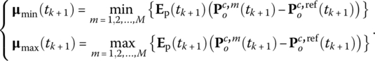
Constraint 2. The second constraint ensures that the image feature parameters in the next time instant ![]() are within the bounds of the envelope of the demonstrated motions. For that purpose, first at each time step, the principal directions of the demonstrated motions are found by utilizing the eigenvectors of the covariance matrix from the demonstrations. For instance, for feature 1, the covariance matrix at each time instant is associated with the concatenated observation vectors from the entire set of demonstrations
are within the bounds of the envelope of the demonstrated motions. For that purpose, first at each time step, the principal directions of the demonstrated motions are found by utilizing the eigenvectors of the covariance matrix from the demonstrations. For instance, for feature 1, the covariance matrix at each time instant is associated with the concatenated observation vectors from the entire set of demonstrations ![]() , i.e.,
, i.e., ![]() . For the set of three trajectories in Figure 6.4a, the eigenvectors ê1, ê2 are illustrated at three different time instants tk for k = 10, 30, 44. The observed image plane features are depicted by different types of markers in Figure 6.4.
. For the set of three trajectories in Figure 6.4a, the eigenvectors ê1, ê2 are illustrated at three different time instants tk for k = 10, 30, 44. The observed image plane features are depicted by different types of markers in Figure 6.4.

Figure 6.4 (a) The eigenvectors of the covariance matrix ê1, ê2 for three demonstrations at times k = 10, 30, and 44; (b) observed parameters for feature 1,  . The vector
  is required to lie in the region bounded by ηmin and ηmax.
The matrix of the eigenvectors Er(tk) rotates the observed image feature vectors along the principal directions of the demonstrated motions. Thus, the observed motion is projected in a local reference frame, aligned with the instantaneous direction of the demonstrations. For instance, the observed parameters for feature 1 of the three demonstrations in the next time instant, ![]() and
and ![]() , are shown rotated in Figure 6.4b, with respect to the reference image feature parameters
, are shown rotated in Figure 6.4b, with respect to the reference image feature parameters ![]() . The rotated observation vectors
. The rotated observation vectors ![]() for
for ![]() define the boundaries of the demonstrated space at the time instant
define the boundaries of the demonstrated space at the time instant ![]() , which corresponds to the hatched section in Figure 6.4b. The inner and outer bounds of the demonstrated envelope are calculated according to
, which corresponds to the hatched section in Figure 6.4b. The inner and outer bounds of the demonstrated envelope are calculated according to

The minimum and maximum operations in (6.17) are performed separately for the horizontal and vertical image coordinates, so that the bounds ![]() and
and ![]() represent 2 × 1 vectors (see Figure 6.4b).
represent 2 × 1 vectors (see Figure 6.4b).
Suppose there exists an unknown vector ![]() related to the image feature parameters in the next time instance. The vector
related to the image feature parameters in the next time instance. The vector ![]() , and its coordinate transformation when rotated in the instantaneous demonstrated direction, is denoted by
, and its coordinate transformation when rotated in the instantaneous demonstrated direction, is denoted by
Then the following constraint ensures that each dimension of ![]() is bounded within the demonstrated envelope:
is bounded within the demonstrated envelope:

The inequalities in (6.19) can be converted to equalities by introducing non‐negative excess (or surplus) and slack variables. In other words, by adding a vector of excess variables ηe to η, and subtracting a vector of slack variables ηs from η, the constraints (6.19) can be represented with the following linear equalities:

Constraint 3. This constraint ensures that the image feature trajectories stay in the FoV of the camera. Therefore, if the image limits in the horizontal direction are denoted as ru, min and ru, max, and the vertical image limits are denoted by rv, min and rv, max, then the coordinates of each feature point should stay bounded within the image limits, that is, the following set of inequalities should hold:

By adding excess and slack variables, the constraints in (6.21) are rewritten as

6.4.5.2 Cartesian Space Constraints
These constraints apply to the object position and velocity in the Cartesian space.
Constraint 1. The relationship between the Cartesian position of the object with respect to the camera frame and the translational (linear) velocity is
In discrete form, (6.23) is represented as
Constraint 2. A constraint is introduced to guarantee that the Cartesian trajectory of the object stays within the envelope of the demonstrated motions in the Cartesian space. This constraint will prevent potential collisions of the object with the surrounding objects in the scene. Note that it is assumed that the demonstrated space defined by the envelope of the demonstrated Cartesian motions is free of obstacles, that is, all the points within the demonstrated envelope are considered safe.
Similar to the image‐based Constraint 2 developed in (6.18)–(6.20), the inner and outer bounds of the demonstrations are found by utilizing the principal directions of the covariance matrix of the demonstrated Cartesian trajectories, i.e.,
For an unknown vector ![]() associated with the position of the object of interest in the next time instant, the distance vector to the reference object position
associated with the position of the object of interest in the next time instant, the distance vector to the reference object position ![]() , rotated by the instantaneous eigenvector matrix, is given by
, rotated by the instantaneous eigenvector matrix, is given by
The components of ![]() are constrained to lie within the bounds of the demonstrated envelope via the following inequality:
are constrained to lie within the bounds of the demonstrated envelope via the following inequality:
where d denotes the dimensionality of the vectors. By introducing excess μe and slack μs variables, the constraint can be represented in the form of equalities

Constraint 3. Another constraint is established for the velocity of the object vo, which is to be bounded between certain minimum and maximum values,
where d is also used for indexing the dimensions of the velocity vector.
By plugging excess and slack variables in (6.29), the following set of equations is obtained:

The values of maximal and minimal velocities, vmax and vmin, could be associated with the extreme values of the velocities that can be exerted by the robot’s end point during the object’s manipulation. Therefore, this constraint can also be categorized into the robot kinematic constraints, presented next.
6.4.5.3 Robot Manipulator Constraints
This set of constraints establishes the relationship between the robot joint angles and the output variable of the optimization model (i.e., the velocity of the target object ![]() ), and introduces a constraint regarding the limitations of the robot’s joints.
), and introduces a constraint regarding the limitations of the robot’s joints.
Constraint 1. The first constraint relates the robot joint variables to the object’s velocity. It is assumed that the object is grasped in the robot’s gripper (Figure 6.3), with the velocity transformation between the object frame expressed in the robot base frame ![]() and robot’s end‐point frame
and robot’s end‐point frame ![]() given by
given by

In (6.31), the notation ![]() is used for the position vector of the object with respect to the end point expressed relative to the robot base frame, whereas
is used for the position vector of the object with respect to the end point expressed relative to the robot base frame, whereas ![]() denotes a skew‐symmetric matrix, which for an arbitrary vector
denotes a skew‐symmetric matrix, which for an arbitrary vector ![]() is defined as
is defined as

The differential kinematic equation of the robot is given with (6.2). Hence, the relationship between the joint variables and the object velocity in camera frame is obtained using (6.31) and (6.2),

where ![]() and
and ![]() are 3 × 3 identity and zeroes matrices, respectively, and J†(q) denotes the pseudoinverse of the robot Jacobian matrix of size
are 3 × 3 identity and zeroes matrices, respectively, and J†(q) denotes the pseudoinverse of the robot Jacobian matrix of size ![]() . At the time tk, (6.33) can be represented in a discrete form
. At the time tk, (6.33) can be represented in a discrete form

The rotation matrix of robot’s end point in base frame ![]() is obtained by using the robot’s forward kinematics. The rotation matrix of the camera frame in robot base frame
is obtained by using the robot’s forward kinematics. The rotation matrix of the camera frame in robot base frame ![]() is found from the calibration of the camera. This matrix is constant, since both the robot’s base frame and the camera frame are fixed. Position of the object frame with respect to the end‐point frame
is found from the calibration of the camera. This matrix is constant, since both the robot’s base frame and the camera frame are fixed. Position of the object frame with respect to the end‐point frame ![]() is also time‐independent, and it is obtained by measurements with a coordinate‐measuring machine.
is also time‐independent, and it is obtained by measurements with a coordinate‐measuring machine.
Constraint 2. A constraint ensuring that the robot joint variables are within the robot workspace limits is defined as
where qmin and qmax stand for the vectors of minimal and maximal realizable values for the joint angles. To represent (6.35) in the form of equalities, excess and slack variables are introduced yielding

6.4.6 Optimization Model
The overall second‐order optimization model is reported in this section in its full form. The model is rewritten in terms of the unknown (decision) variables, and the known variables and parameters, at each instance of the optimization procedure.
Recall that the objective function is defined in (6.14). The model constraints include the following: the linear constraints defining the relations between the variables given with (6.16), (6.18), (6.24), (6.26), and (6.34); the linear constraints obtained from inequalities by introducing excess and slack variables given with (6.20), (6.22), (6.28), (6.30), and (6.36); and the conic constraints given with (6.12) and (6.13). Also, non‐negativity constraints for the components of all excess and slack variables are included in the model.
Auxiliary variables are introduced that denote the difference between the image parameters and the reference image features for the feature n at the next time instant, ![]() . Accordingly, the corresponding image feature vector is obtained by stacking the variables for each image feature,
. Accordingly, the corresponding image feature vector is obtained by stacking the variables for each image feature, ![]() . Thus, subtracting the term
. Thus, subtracting the term ![]() on both sides of (6.16) results in
on both sides of (6.16) results in
With rearranging the given equation, it can be rewritten in terms of the unknown variables in the model ![]() and
and ![]() , and the known variables at the time instant tk, that is, ξ(tk), L(tk),
, and the known variables at the time instant tk, that is, ξ(tk), L(tk), ![]() , and Δtk
, and Δtk

Similarly, (6.18) is rewritten in terms of the introduced variables

Analogous to (6.38), by introducing an auxiliary variable ![]() , and subtracting
, and subtracting ![]() from both sides of (6.24), it becomes
from both sides of (6.24), it becomes

whereas (6.26) can also be rewritten in terms of the unknown variables

In these equations, the variables ![]() ,
, ![]() , and
, and ![]() are known.
are known.
Similarly, (6.34) can be rewritten as

The linear constraints related to the excess and slack variables in (6.20), (6.22), (6.28), (6.30), and (6.36) can be represented in a similar form as


The conic constraint (6.12) can also be rewritten in a similar fashion as
The other conic constraints (6.13) can be written as

where auxiliary variables for the linear and angular velocity are introduced as ![]() and
and ![]() , respectively, that is,
, respectively, that is,

The non‐negativity constraints for the excess and slack variables yield

To summarize, the optimization variable z in (6.11) at the time instant tk is formed by concatenation of the variables from the conic constraints (6.48) and (6.49)
and the variables from the linear constraints
that is, ![]() . The size of the component zc(tk) is
. The size of the component zc(tk) is ![]() , whereas the size of the component zl(tk) is
, whereas the size of the component zl(tk) is ![]() .
.
From the cost function defined in (6.14)

the part of the vector c in (6.11) that corresponds to the zc(tk) is
whereas the part cl(tk) corresponding to zl(tk) is all zeros, since those variables are not used in the cost function.
The known parameters for the optimization model at time tk are as follows: Δtk, ξ(tk), ![]() , L(tk),
, L(tk), ![]() ,
, ![]() ,
, ![]() ,
, ![]() , q(tk),
, q(tk), ![]() , J†(q(tk)),
, J†(q(tk)), ![]() ,
, ![]() ,
, ![]() ,
, ![]() ,
, ![]() , and the time‐independent parameters: rmin, rmax, vmin, vmax, qmin, qmax,
, and the time‐independent parameters: rmin, rmax, vmin, vmax, qmin, qmax, ![]() , and
, and ![]() .
.
The problem can be solved as second‐order conic minimization because the relations among the variables and the parameters are formulated as linear and conic constraints. A series of the presented minimization procedure is performed at each time instant tk. The important unknown variables of the model at times tk are the object velocity ![]() and the locations of the features points at the next time instant
and the locations of the features points at the next time instant ![]() . By tuning the weighting coefficients α’s in the objective function, the results can be adjusted to follow more closely the reference image trajectories, or the reference object velocities, as explained in the sequel.
. By tuning the weighting coefficients α’s in the objective function, the results can be adjusted to follow more closely the reference image trajectories, or the reference object velocities, as explained in the sequel.
6.5 Robust Image‐Based Tracking Control
To follow the image feature trajectories ξ(tk) for ![]() generated from the optimization model, an image‐based visual tracker is employed. The control ensures that the errors between the measured feature parameters
generated from the optimization model, an image‐based visual tracker is employed. The control ensures that the errors between the measured feature parameters ![]() and the desired feature parameters ξ, that is,
and the desired feature parameters ξ, that is, ![]() , are driven to zero for
, are driven to zero for ![]() . By taking derivative of the error and using (6.15), a relation between the features error and the object velocity is established as follows:
. By taking derivative of the error and using (6.15), a relation between the features error and the object velocity is established as follows:
A controller with exponential decoupled decrease of the error ![]() is a common choice in solving visual servoing problems, thus it is adopted here as well. Therefore, (6.55) yields
is a common choice in solving visual servoing problems, thus it is adopted here as well. Therefore, (6.55) yields
where ![]() is an approximation of the pseudoinverse of the image Jacobian matrix L(t). The applied control law warrants that when the error between the measured and the followed feature parameters is small, the velocity of the object will follow closely the desired velocity generated by the optimization model. Note that the image Jacobian matrix L(t) requires information that is not directly available from the image measurements, for example, partial pose estimation of the object. Therefore, an approximation of the matrix is usually used in visual servoing tasks, with different models for the approximation reported in the literature (Chaumette and Hutchinson, 2007).
is an approximation of the pseudoinverse of the image Jacobian matrix L(t). The applied control law warrants that when the error between the measured and the followed feature parameters is small, the velocity of the object will follow closely the desired velocity generated by the optimization model. Note that the image Jacobian matrix L(t) requires information that is not directly available from the image measurements, for example, partial pose estimation of the object. Therefore, an approximation of the matrix is usually used in visual servoing tasks, with different models for the approximation reported in the literature (Chaumette and Hutchinson, 2007).
Regarding the stability of the presented control scheme, it is well known that local asymptotic stability is guaranteed in the neighborhood of ![]() if
if ![]() is positive definite (Chaumette and Hutchinson, 2006). Global asymptotic stability of this type of control cannot be achieved, because the matrix
is positive definite (Chaumette and Hutchinson, 2006). Global asymptotic stability of this type of control cannot be achieved, because the matrix ![]() has a nonzero null space. However, in the neighborhood of the desired pose, the control scheme is free of local minima and the convergence is guaranteed (Chaumette and Hutchinson, 2006). These properties of the IBVS control render its suitability for tracking tasks, such as the problem at hand. That is, when the features selection and system calibration are reasonably performed so that
has a nonzero null space. However, in the neighborhood of the desired pose, the control scheme is free of local minima and the convergence is guaranteed (Chaumette and Hutchinson, 2006). These properties of the IBVS control render its suitability for tracking tasks, such as the problem at hand. That is, when the features selection and system calibration are reasonably performed so that ![]() is positive definite, then the errors between the current and desired feature parameters will converge to zero along the tracked trajectory. Although the region of local asymptotic stability is difficult to be calculated theoretically, it has been shown that, in practice, it can be quite large (Chaumette and Hutchinson, 2006).
is positive definite, then the errors between the current and desired feature parameters will converge to zero along the tracked trajectory. Although the region of local asymptotic stability is difficult to be calculated theoretically, it has been shown that, in practice, it can be quite large (Chaumette and Hutchinson, 2006).
For calculations of the robot joint angles for the task execution, the robot Jacobian matrix is combined with the image Jacobian matrix into a feature Jacobian matrix ![]() (Chaumette and Hutchinson, 2007)
(Chaumette and Hutchinson, 2007)

which provides a direct mapping between the image feature parameters and the time change of the joint angle variables, that is, ![]() . The joint angles of the robot are updated based on (6.33) and (6.56), i.e.,
. The joint angles of the robot are updated based on (6.33) and (6.56), i.e.,
which in discrete form becomes
6.5.1 Simulations
The presented approach is first evaluated through simulations in a virtual environment. The goal of the simulations is mainly to verify the developed task planning method in the image space via the presented optimization model. In the next section, the approach is subjected to more thorough evaluations through experiments with a robot in a real‐world environment.
The simulations and the experiments were performed in the MATLAB environment on a 3‐GHz quad‐core CPU with 4‐GB of RAM running under Windows 7 OS.
A simulated environment in MATLAB was created using functions from the visual servoing toolbox for MATLAB/Simulink (Cervera, 2003) and the Robotics toolbox for MATLAB (Corke, 2011). The conic optimization is solved by using the SeDuMi software package (Sturm, 1997).
A virtual camera model is created, corresponding to the 640 × 480 pixels Point Grey’s Firefly®MV camera, introduced in Section 2.2. A virtual robot Puma 560 is adopted for execution of the generated reproduction strategy. Nonetheless, the focus of the simulations is on the task planning, rather than the task execution.
The simulations are carried out for two different types of demonstrated motions. Simulation 1 uses synthetic generated trajectories, whereas Simulation 2 employs human‐executed trajectories. The discrete sampling period for both simulations is set equal to ![]() seconds, for
seconds, for ![]() .
.
Note that in Figures 6.5–6.14, the plots depicting the image plane of the camera are displayed with borders around them, in order to be easily differentiated from the time plots of the other variables, such as Cartesian positions or velocities. The image feature parameters in the figures are displayed in pixel coordinates ![]() , rather than in spatial coordinates
, rather than in spatial coordinates ![]() , since it is more intuitive for presentation purposes. The demonstrated trajectories are depicted with thin solid lines (unless otherwise indicated). The initial states of the trajectories are indicated by square marks, while the final states are indicated by cross marks. In addition, the reference trajectories obtained from Kalman smoothing are represented by thick dashed lines, and the generalized trajectories obtained from the conic optimization are depicted by thick solid lines. The line styles are also described in the figure legends.
, since it is more intuitive for presentation purposes. The demonstrated trajectories are depicted with thin solid lines (unless otherwise indicated). The initial states of the trajectories are indicated by square marks, while the final states are indicated by cross marks. In addition, the reference trajectories obtained from Kalman smoothing are represented by thick dashed lines, and the generalized trajectories obtained from the conic optimization are depicted by thick solid lines. The line styles are also described in the figure legends.


Figure 6.5 (a) Three demonstrated trajectories of the object in the Cartesian space. For one of the trajectories, the initial and ending coordinate frames of the object are shown, along with the six coplanar features; (b) projected demonstrated trajectories of the feature points onto the image plane of the camera; (c) reference image feature trajectories produced by Kalman smoothing and generalized trajectories produced by the optimization model; and (d) object velocities from the optimization model.


Figure 6.6 (a) Demonstrated Cartesian trajectories of the object, with the features points, and the initial and ending object frames; (b) demonstrated and reference linear velocities of the object for x‐ and y‐coordinates of the motions; (c) reference image feature trajectories from the Kalman smoothing and the corresponding generalized trajectories from the optimization; and (d) the demonstrated and retrieved generalized object trajectories in the Cartesian space. The initial state and the ending state are depicted with square and cross marks, respectively.

Figure 6.7 (a) Experimental setup showing the robot in the home configuration and the camera. The coordinate axes of the robot base frame and the camera frame are depicted; (b) the object with the coordinate frame axes and the features.

Figure 6.8 Sequence of images from the kinesthetic demonstrations.


Figure 6.9 (a) Feature trajectories in the image space for one‐sample demonstration; (b) demonstrated trajectories, Kalman‐smoothed (reference) trajectory, and corresponding planned trajectory for one feature point (for the feature no. 2); (c) demonstrated linear and angular velocities of the object and the reference velocities obtained by Kalman smoothing; (d) Kalman‐smoothed (reference) image feature trajectories and the generalized trajectories obtained from the optimization procedure; and (e) demonstrated and the generated Cartesian trajectories of the object in the robot base frame.


Figure 6.10 (a) Desired and robot‐executed feature trajectories in the image space; (b) tracking errors for the pixel coordinates (u, v) of the five image features in the image space; (c) tracking errors for x‐, y‐, and z‐coordinates of the object in the Cartesian space; (d) translational velocities of the object from the IBVS tracker.


Figure 6.11 Task execution without optimization of the trajectories: (a) Desired and robot‐executed feature trajectories in the image space; (b) tracking errors for the pixel coordinates (u, v) of the five image features in the image space; (c) tracking errors for x‐, y‐, and z‐coordinates of the object in the Cartesian space; (d) translational velocities of the object from the IBVS tracker.

Figure 6.12 (a) Demonstrated trajectories of the image feature points, superimposed with the desired and robot‐executed feature trajectories; (b) desired and executed trajectories for slowed down trajectories.


Figure 6.13 (a) Image feature trajectories for one of the demonstrations; (b) demonstrated trajectories, reference trajectory from the Kalman smoothing, and the corresponding generalized trajectory for one of the feature points; (c) desired and robot‐executed image feature trajectories; (d) translational velocities of the object from the IBVS tracker; (e) tracking errors for pixel coordinates (u, v) of the five image features in the image space; and (f) tracking errors for x‐, y‐, and z‐coordinates of the object in the Cartesian space.

Figure 6.14 Projected trajectories of the feature points in the image space with (a) errors of 5, 10, and 20% introduced for all camera intrinsic parameters; (b) errors of 5% introduced for the focal length scaling factors of the camera.
6.5.1.1 Simulation 1
This simulation case is designed for initial examination of the planning in a simplistic scenario with three synthetic trajectories of a moving object generated in MATLAB. The Cartesian positions of the object are shown in Figure 6.5a. For one of the demonstrated trajectories, the axes of the coordinate frame of the object are also shown in the plot. A total rotation of 60° around the y‐axis has been applied to the object during the motion. The motions are characterized by constant velocities. Six planar features located on the object are observed by a stationary camera (i.e., ![]() ). The projections of the feature points onto the image plane of the camera for the three demonstrations are displayed in Figure 6.5b with different line styles. The boundaries of the task in the Cartesian and image space can be easily inferred for the demonstrated motions. The simulation scenario is designed such that there is a violation of the FoV of the camera. Note that in the simulations the FoV of the camera is infinite, that is, negative values of the pixels can be handled.
). The projections of the feature points onto the image plane of the camera for the three demonstrations are displayed in Figure 6.5b with different line styles. The boundaries of the task in the Cartesian and image space can be easily inferred for the demonstrated motions. The simulation scenario is designed such that there is a violation of the FoV of the camera. Note that in the simulations the FoV of the camera is infinite, that is, negative values of the pixels can be handled.
Kalman smoothers are employed to find smooth average trajectories for each feature point r(n),ref, as well as to find the reference velocities of the object ![]() . For initialization of the Kalman smoothers, the measurement and process noise covariance matrices are set as follows. For the image feature parameters corresponding to each feature point n:
. For initialization of the Kalman smoothers, the measurement and process noise covariance matrices are set as follows. For the image feature parameters corresponding to each feature point n: ![]() ,
, ![]() ; for the object’s pose:
; for the object’s pose: ![]() ,
, ![]() ; and for the object’s linear and angular velocities:
; and for the object’s linear and angular velocities: ![]() ,
, ![]() . As noted before, the notation
. As noted before, the notation ![]() refers to an identity matrix of size a. The resulting reference trajectories for the image features are depicted with dashed lines in Figure 6.5c. It can be noticed that for some of the feature points, a section of the reference trajectories is outside of the image boundaries.
refers to an identity matrix of size a. The resulting reference trajectories for the image features are depicted with dashed lines in Figure 6.5c. It can be noticed that for some of the feature points, a section of the reference trajectories is outside of the image boundaries.
The optimization model constraints (6.22) ensure that all image features stay within the camera FoV during the entire length of the motion. The image boundaries in this case are defined as ±10 pixels from the horizontal and vertical dimensions of the image sensor, that is,

Accordingly, a series of second‐order conic optimization models described in Section 6.4.6 is run, with the reference trajectories from the Kalman smoothing algorithms used as inputs for the optimizations. The following values for the weighting coefficients were adopted: ![]() and
and ![]() . The resulting image feature trajectories from the optimization are depicted with thick solid lines in Figure 6.5c, whereas the resulting velocity of the object is shown in Figure 6.5d. The angular velocities around the x‐ and z‐axes are zero and therefore are not shown in the figure. It can be observed in Figure 6.5c that the image feature trajectories are confined within the FoV bounds defined in (6.60). For the image feature parameters that have values less than the specified boundary for the vertical coordinate, that is,
. The resulting image feature trajectories from the optimization are depicted with thick solid lines in Figure 6.5c, whereas the resulting velocity of the object is shown in Figure 6.5d. The angular velocities around the x‐ and z‐axes are zero and therefore are not shown in the figure. It can be observed in Figure 6.5c that the image feature trajectories are confined within the FoV bounds defined in (6.60). For the image feature parameters that have values less than the specified boundary for the vertical coordinate, that is, ![]() pixels, the presented approach modified the plan to satisfy the image limits constraint.
pixels, the presented approach modified the plan to satisfy the image limits constraint.
6.5.1.2 Simulation 2
This simulation entails a case where an object is moved by a human demonstrator, while the poses of the object are recorded with an optical marker‐based tracker. A total of five demonstrations are collected, displayed in Figure 6.6. The demonstrations involve translatory motions, whereas synthetic rotation of 60° around the y‐axis has been added to all trajectories. It is assumed that the object has six point features and the model of the object is readily available. Different from Simulation 1, the demonstrated trajectories in Simulation 2 are characterized by the nonconsistency of human‐demonstrated motions. The velocities of the demonstrated trajectories are shown in Figure 6.6b. The Kalman‐smoothed velocities of the object are shown with the dashed lines in Figure 6.6b. Similarly, the smoothed image feature trajectories are given in Figure 6.6c. The same initialization parameters for the Kalman smoothers as in Simulation 1 were employed.
The resulting reference trajectories are then used for initialization of the optimization procedure. Similar to Simulation 1, the weighting coefficients are set to ![]() and
and ![]() . The weighting scheme assigns higher weight to the importance of following the reference velocities, whereas the model constraints ensure that the generated feature trajectories in the image space are close to the reference trajectories and are within the bounds of the demonstrated task space. As a result, the generated object velocities vo are almost identical to the reference velocities shown in Figure 6.6b. The generated image feature trajectories are shown with the thick lines in Figure 6.6c. The corresponding Cartesian object trajectory is shown in Figure 6.6d. The trajectory is within the bounds of the demonstrated task space, and reaching the final goal state of the task is accomplished. The simulation results of the robot’s task execution are not presented, since a more proficient analysis is provided in the next section, involving real‐world experiments.
. The weighting scheme assigns higher weight to the importance of following the reference velocities, whereas the model constraints ensure that the generated feature trajectories in the image space are close to the reference trajectories and are within the bounds of the demonstrated task space. As a result, the generated object velocities vo are almost identical to the reference velocities shown in Figure 6.6b. The generated image feature trajectories are shown with the thick lines in Figure 6.6c. The corresponding Cartesian object trajectory is shown in Figure 6.6d. The trajectory is within the bounds of the demonstrated task space, and reaching the final goal state of the task is accomplished. The simulation results of the robot’s task execution are not presented, since a more proficient analysis is provided in the next section, involving real‐world experiments.
6.5.2 Experiments
Experimental evaluation of the approach is conducted with a CRS A255 desktop robot and a Point Grey’s Firefly MV camera (Section 2.2), both shown in Figure 6.7a. An object with five coplanar circular features shown in Figure 6.7b is used for the experiments. The centroids of the circular features are depicted with cross markers in the figure, and also the circular features are circumscribed with solid lines. The coordinates of the centroids of the dots in the object frame are (12, 22, 0), (−12, 22, 0), (0, 0, 0), (−12, −22, 0), and (12, −22, 0) millimeters. The demonstrations consist of manipulating the object in front of the camera.
The frame rate of the camera was set to 30 fps. A megapixel fixed focal length lens from Edmund Optics Inc. was used. The camera was calibrated by using the camera calibration toolbox for MATLAB® (Bouguet, 2010). The calibration procedure uses a set of 20 images of a planar checkerboard taken at different positions and orientations with respect to the camera. The camera parameters are estimated employing nonlinear optimization (based on iterative gradient descent) for minimizing the radial and tangential distortion in the images. The calibration estimated values of the intrinsic camera parameters are as follows: principal point coordinates ![]() ,
, ![]() pixels, focal length
pixels, focal length ![]() millimeters, and the scaling factors
millimeters, and the scaling factors ![]() ,
, ![]() pixels.
pixels.
The CRS A255 robot is controlled through the QuaRC toolbox for open‐architecture control (QuaRC, 2012). In fact, the CRS A255 robot was originally acquired as a closed‐architecture system, meaning that prestructured proportional–integral–derivative (PID) feedback controllers are employed for actuating the links’ joints. For example, when a user commands the robot to move to a desired position, the built‐in PID controllers calculate and send current to joint motors, in order to drive the robot to the desired position. That is, the closed‐architecture controller prevents the users from accessing the joint motors and implementing advanced control algorithms. On the other hand, the QuaRC toolbox for open architecture, developed by Quanser (Markham, Ontario), allows direct control of the joint motors of the CRS robot. It uses Quanser Q8 data‐acquisition board for reading the joint encoders and for communicating with the motor amplifiers at 1‐millisecond intervals. In addition, QuaRC provides a library of custom Simulink blocks and S‐functions developed for the A255 robot, thus enabling design of advanced control algorithms and real‐time control of the robot motions in Simulink environment. The toolbox also contains a block for acquisition of images with Point Grey’s FireflyMV camera.
The A255 robot has an anthropomorphic structure, that is, it is realized entirely by revolute joints, and by analogy to the human body, it consists of an arm and a wrist. The arm of the A255 manipulator endows three DoFs, whereas the wrist provides two DoFs. The fact that the wrist has only two DoFs prevents from exerting arbitrary orientation of the robot’s end point, and subsequently an arbitrary orientation of the manipulated object cannot be achieved. Accordingly, the experiments are designed to avoid the shortcomings of the missing rotational DoF. In the first place, one must have in mind that human‐demonstrated trajectories cannot be completely devoid of a certain rotational DoF, due to the stochastic character of human motion. Therefore, kinesthetic demonstrations are employed for the experiments (see Figure 6.8), meaning that while the object is grasped by the robot’s gripper, the joint motors are set into passive mode, and the links are manually moved by a demonstrator (Hersch et al., 2008; Kormushev et al., 2011). Furthermore, the kinesthetic mode of demonstrations does not require solving the correspondence problem between the embodiments of the demonstrator and the robot. The drawbacks are related to the reduced naturalness of the motions, and also this demonstration mode can be challenging for robots with large number of DoFs.
Three sets of experiments are designed to evaluate the performance of the presented approach.
6.5.2.1 Experiment 1
The first experiment consists of moving an object along a trajectory of a pick‐and‐place task. A sequence of images from the kinesthetic demonstrations is displayed in Figure 6.8. The total number of demonstrated trajectories M is 5. Image plane coordinates of the centroids of the dots are considered as image feature parameters, denoted by ![]() . The trajectories of the feature points in the image plane of the camera for one of the demonstrations are presented in Figure 6.9a. As explained, the initial and ending states are illustrated with square and cross marks, respectively.
. The trajectories of the feature points in the image plane of the camera for one of the demonstrations are presented in Figure 6.9a. As explained, the initial and ending states are illustrated with square and cross marks, respectively.
Tracking the features in the acquired image sequences is based on the “dot tracker” method reported in the VISP package (Marchand et al., 2005). More specifically, before the manipulation task, with the robot set in the initial configuration, the five dots on the object are manually selected in an acquired image. Afterward, tracking of each feature is achieved by processing a region of interest with a size of 80 pixels, centered at the centroid of the dot from the previous image. The feature extraction involved binarization, thresholding, and centroids calculation of the largest blobs with connected pixels in the windows. The extracted trajectories are initially lightly smoothed with a moving average window of three points, and linearly scaled to the length of the longest demonstration (which was equal to 511 frames for the considered experiment). Consequently, the demonstrated input data in the image plane coordinates form the set ![]() for
for ![]() ,
, ![]() ,
, ![]() . Recall that, in the figures, the image features are shown in pixel coordinates
. Recall that, in the figures, the image features are shown in pixel coordinates ![]() , for more intuitive presentation.
, for more intuitive presentation.
For the Kalman smoothing, the measurement and process noise covariance matrices corresponding to the image feature parameters are ![]() and
and ![]() , respectively. For the object’s pose, the corresponding matrices are
, respectively. For the object’s pose, the corresponding matrices are ![]() ,
, ![]() , and for the object’s velocities are
, and for the object’s velocities are ![]() ,
, ![]() . The initialization based on the given parameters imposes greater smoothing on the Cartesian position and velocity data, since these parameters are calculated indirectly from the noisy image measurements (by using planar homography transformation). The demonstrated and the reference velocities are shown in Figure 6.9c. On the other hand, the selected initialization for the image feature trajectories results in tight following of the demonstrated trajectories in the image space. The smooth average trajectory from the Kalman smoothing for the feature point 2 (i.e., u(2),ref) is depicted by the thick dashed line in Figure 6.9b.
. The initialization based on the given parameters imposes greater smoothing on the Cartesian position and velocity data, since these parameters are calculated indirectly from the noisy image measurements (by using planar homography transformation). The demonstrated and the reference velocities are shown in Figure 6.9c. On the other hand, the selected initialization for the image feature trajectories results in tight following of the demonstrated trajectories in the image space. The smooth average trajectory from the Kalman smoothing for the feature point 2 (i.e., u(2),ref) is depicted by the thick dashed line in Figure 6.9b.
Afterward, the optimization procedure described in Section 6.4 is performed. The discrete sampling period is set to ![]() seconds (which corresponds to the camera frame rate), for
seconds (which corresponds to the camera frame rate), for ![]() . The adopted values for the weighting coefficients,
. The adopted values for the weighting coefficients, ![]() and
and ![]() , assign higher weights on the importance for emulating the reference velocities. Less emphasis is placed on following the reference image trajectories. The overall computational time for solving the optimization procedures for this experiment was approximately 30 seconds. The output trajectory from the optimization step is shown in pixel coordinates in Figure 6.9b for the feature point 2 with a thick solid line, superimposed with the demonstrated trajectories and the reference trajectory. Additionally, the output image trajectories for all five feature points are shown in Figure 6.9d, and the corresponding Cartesian trajectory of the object expressed in the robot base frame is shown in Figure 6.9e.
, assign higher weights on the importance for emulating the reference velocities. Less emphasis is placed on following the reference image trajectories. The overall computational time for solving the optimization procedures for this experiment was approximately 30 seconds. The output trajectory from the optimization step is shown in pixel coordinates in Figure 6.9b for the feature point 2 with a thick solid line, superimposed with the demonstrated trajectories and the reference trajectory. Additionally, the output image trajectories for all five feature points are shown in Figure 6.9d, and the corresponding Cartesian trajectory of the object expressed in the robot base frame is shown in Figure 6.9e.
In Figure 6.9b, it is noticeable that the reference trajectory obtained by the Kalman smoother (the dashed line) does not correspond to the geometric mean of the demonstrations, and at some points, it does not belong to the envelope of the demonstrated trajectories. The reason behind this is the temporal variations across the trajectories due to the random distributions of velocities in the demonstrations, that is, the trajectories are linearly scaled to an equal length, but they are not temporally scaled. Therefore, the observed features locations at particular time instants tk correspond to different states (i.e., spatial positions) across the demonstrated set of M trajectories. On the other hand, it can be noticed that the generated trajectory from the second‐order conic optimization is constrained to lie within the envelope of the demonstrated trajectories. One could note here that if the demonstrated trajectories were temporally scaled (for instance, by using the DTW algorithm described in Section 3.3.2), the resulting reference trajectories of the features points would be bounded within the demonstrated envelope, thus they would be better representatives of the task. However, the disadvantage of this approach is the distortion of the velocity profile of the demonstrations caused by the temporal warping, and therefore, it is not considered for the problem at hand.
To move the object by the robot along the generalized trajectory from the optimization model, the IBVS tracking control from (6.58) is employed. The control is implemented through the QuaRC open‐architecture system with a rate of 33 milliseconds, while the internal loop for low‐level control of the joint motors operates at 1 millisecond rate. The resulting trajectories of the object features during the task execution by the robot are shown in Figure 6.10a (the line with circle markers). For comparison, the desired trajectories from the optimization process are also shown in the figure, depicted with thick solid lines. Regarding the selection of the control gain λ, recall that higher gains dictate fast adaptation to the desired trajectory accompanied with reduced accuracy due to overshoots, and vice versa for the lower control gains. Also, setting the control gain too high can destabilize the system. Thus, initially the performance of the system was evaluated for different values of the control gain. Subsequently, for the parameter λ, the value of 0.75 was adopted for the first 4/5th of the trajectory length—in order to ensure accurate tracking, and the value of 0.1 was adopted for the last 1/5th of the trajectory—to provide accurate positioning at the end of the task. The tracking errors in the image plane are shown in Figure 6.10b, for the horizontal (u) and vertical (v) pixel coordinates of the five features. The errors during the trajectory following are moderate, with values in the range of several pixels, and with the errors at the final position settling within 2 pixels. The tracking errors in the Cartesian space are shown in Figure 6.10c. The steady‐state errors at the final object position expressed in the robot base frame are (1.05, 0.04, −0.15) millimeters. The x‐coordinate corresponds to the depth measurements in the camera frame. As expected, feature depths are more sensitive to image noise, due to the camera projection model. The command values for the linear velocities of the object are shown in Figure 6.10d.
The presented approach is important because it establishes a framework for exploiting the robustness of vision‐based control in PbD learning. For instance, consider the trajectory tracking results shown in Figure 6.11, which correspond to the same object manipulation task, but this time the reference trajectories from the Kalman smoother are used as desired trajectory for the IBVS tracking. In other words, the optimization procedure was not performed. The results indicate that the tracking is less successful (Figure 6.11a), yielding steady‐state image‐space errors of approximately 5 pixels (Figure 6.11b). Moreover, the object position at the end of the task (Figure 6.11c) implies divergence from the desired position, as well as high command velocities at the beginning of the tracking (Figure 6.11d). These results reveal the difficulties associated with the trajectory planning in the image space due to nonlinearity in the mapping between the image space and the Cartesian space. More specifically, the positions of the five feature points in the image plane may not necessarily correspond to a realizable Cartesian pose of the object, and/or they may impose large velocities of the object in the Cartesian space. In the considered case, the final positions of the image feature parameters are not achievable, that is, there exist steady‐state errors in the image space that the control scheme attempts to minimize, which result in the task failure with regards to the final Cartesian position of the object (Figure 6.11c).
6.5.2.2 Experiment 2
The second experiment is designed to evaluate the performance of the presented approach for trajectories with sharp turns, with the results presented in Figure 6.12. The task is repeated four times by a human teacher via kinesthetic demonstrations. The trajectory learning is performed using the same learning parameters as in Experiment 1. The robot‐executed trajectory shown in Figure 6.12a indicates overshoots of the desired feature trajectories at the two corners where the sharp turns occur. If the control gain λ was set to lower values, the overshoots could have been avoided but on account of cutting the corners. Figure 6.12b shows the task reproduction by the robot, in the case when the generated desired trajectory is interpolated to a trajectory three times longer than the initial trajectory, that is, this corresponds to slowing down the trajectory three times. In this case, the trajectory following is performed without deviations from the desired trajectory. It can be concluded that the visual tracking performs better for slower trajectories, while fast changing trajectories produce higher tracking errors.
6.5.2.3 Experiment 3
The third experiment is designed to evaluate the tasks involving trajectories with intersecting parts, which is often a challenging case for learning (Khansari‐Zadeh and Billard, 2011). A loop in the demonstrated task is shown in the image plane trajectories in Figure 6.13a. The results from the trajectory planning step with four demonstrations are displayed in Figure 6.13b. Similar to the case with sharp turns in Experiment 2, the presence of the loop caused tracking errors for that part of the trajectory, and therefore the desired trajectory was interpolated to a three times longer trajectory. The result of the tracking in this case is given in Figure 6.13c. The image plane steady‐state errors of the IBVS tracking are within 1.5 pixels (Figure 6.13e), while the translational steady‐state errors of the object in the Cartesian space are (2.4, −0.3, −0.1) millimeters (Figure 6.13f). The results from the task planning and execution steps are satisfactory with small trajectory following errors and small positioning errors of the object at the end of the task.
6.5.3 Robustness Analysis and Comparisons with Other Methods
The advantages of image‐based control stemming from the robustness to modeling errors are next evaluated for several types of uncertainties. First, the outcome of the learning from demonstration process is examined under the assumption that the camera is not properly calibrated. The errors in the intrinsic camera parameters ε ranging from 5 to 80% are introduced for all considered intrinsic parameters as follows: ![]() ,
, ![]() ,
, ![]() , and
, and ![]() . Obviously, these calibration errors affect the transformation in (2.1), that is, the transformation of the measurements from pixel coordinates into the spatial image plane coordinates. In particular, the estimation of the object pose from image coordinates obtained under camera model errors produces erroneous results. In image‐based tracking, the control law operates directly over parameters in the image space and compensates for these errors.
. Obviously, these calibration errors affect the transformation in (2.1), that is, the transformation of the measurements from pixel coordinates into the spatial image plane coordinates. In particular, the estimation of the object pose from image coordinates obtained under camera model errors produces erroneous results. In image‐based tracking, the control law operates directly over parameters in the image space and compensates for these errors.
The robot performance is evaluated using the optical motion capture system Optotrak (Section 2.1). Optical markers are attached onto the object (see Figures 6.4 and 6.7), enabling high accuracy in the measurements of object’s poses over time, in comparison to the estimated poses from camera‐acquired images.
The following comparison parameters are used for quantifying the deviation between the demonstrated trajectories and the robot‐executed trajectories:
- Steady‐state errors of the object’s position:
 , where for each coordinate
  , ξss denotes the steady‐state position of the robot‐executed trajectory, and
  denotes the mean steady‐state position from the set of M demonstrated trajectories
 - RMS deviations for each coordinate
 (6.61)
- Overall RMS deviations, obtained by summing the deviations for all three coordinates
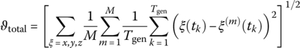
For the IBVS tracking, the values of the parameters are shown in Table 6.1. The results demonstrate the robustness of the IBVS scheme, since even for very large intrinsic errors, for example, 80%, the performance of the tracking is almost unchanged. The errors in the object’s position at the end of the task are in submillimeter amounts for the y‐ and z‐coordinates. For the x‐coordinate of object’s position, the errors are larger, since the x‐axis corresponds to the depth coordinate of the camera. Even with a well‐calibrated camera (i.e., 0% intrinsic errors in the table), the reference values of the steady‐state errors are approximately 8 millimeters. When errors in the intrinsic camera parameters are introduced, the positioning of the object at the end of the task is almost unchanged. Similarly, the tracking errors, quantified with the RMS metrics in Table 6.1, indicate that the trajectory following under intrinsic camera errors is comparable to the performance without introducing intrinsic camera errors. Moreover, the total RMS deviations reveal slightly lower deviations for the case when 10% intrinsic errors are introduced, which may be attributed to the random noise in the image measurements.
Table 6.1 Evaluation of the trajectory tracking with IBVS under intrinsic camera parameters errors ranging from 0 to 80%.
| Intrinsic errors (%) | Steady‐state errors | RMS errors | Total RMS errors | ||||
| x | y | z | x | y | Z | ||
| 0 | 8.2 | 0.2 | 0.4 | 11.1 | 9.3 | 5.3 | 15.4 |
| 5 | 8.3 | 0.1 | 0.5 | 10.8 | 8.8 | 4.8 | 14.7 |
| 10 | 8.3 | 0.04 | 0.5 | 9.4 | 7.8 | 3.8 | 12.8 |
| 20 | 8.6 | 0.02 | 0.7 | 10.5 | 8.3 | 4.1 | 13.9 |
| 40 | 8.4 | 0.1 | 0.6 | 10.3 | 7.6 | 3.5 | 13.3 |
| 80 | 10.6 | 0.6 | 0.7 | 18.7 | 12.1 | 6.4 | 23.2 |
Tracking errors are expressed in millimeters.
For comparison, the task execution is repeated without vision‐based control, that is, the robot uses its motor encoder readings for following a desired trajectory in order to relocate the object. The demonstrated object trajectories in the Cartesian space are extracted from the camera‐sourced images. Two PbD methods are employed for generating a generalized trajectory: (i) Gaussian mixture model/Gaussian mixture regression (GMM/GMR) approach (Calinon, 2009) with eight mixtures of Gaussians used for modeling the demonstrated object positions, and (ii) dynamic motion primitives (DMPs) approach (Ijspeert et al., 2003) with 20 Gaussian kernels used. Velocities of the object in the Cartesian space are used as command inputs for the robot in order to move the object along the generalized trajectories. Subsequently, an operational space velocity controller for the robot’s motion is employed in both cases, based on an inverse differential kinematics scheme (Sciavicco and Siciliano, 2005). The deviations between the demonstrated trajectories and the robot‐executed trajectories measured by the optical tracker are given in Table 6.2. The results indicate deteriorated performance, with high tracking errors, as well as errors in the object positioning at the end of the task. The deviations of the robot‐executed trajectories from the demonstrated trajectories originate from two sources: the object pose estimation using erroneous camera parameters and errors due to robot kinematics. Namely, even for the case without errors in the intrinsic camera parameters (first row in Table 6.2 with 0% errors), there exist tracking and steady‐state position errors due to the robot kinematics (such as incorrect estimate of the robot’s end‐point position after the homing, coupling of the robot’s joints, backlashes, and frictions in the actuators). On the other hand, by using visual feedback to control the robot directly in the image space of the camera, the errors associated with the inaccuracies in the robot kinematic model are avoided.
Table 6.2 Evaluation of the trajectory tracking without vision‐based control under intrinsic camera parameters errors ranging from 0 to 80%.
| Intrinsic errors (%) | GMM/GMR approach | DMPs approach | ||||||
| Steady‐state errors | Total RMS errors | Steady‐state errors | Total RMS errors | |||||
| X | y | Z | x | Y | z | |||
| 0 | 6.5 | 3.4 | 17.0 | 17.7 | 4.2 | 1.5 | 13.3 | 18.6 |
| 5 | 11.7 | 5.0 | 18.2 | 19.1 | 10.2 | 3.0 | 14.8 | 20.3 |
| 10 | 15.9 | 6.8 | 20.2 | 26.5 | 15.7 | 5.2 | 16.4 | 23.4 |
| 20 | 22.3 | 9.62 | 22.5 | 29.9 | 28.5 | 9.6 | 19.6 | 32.4 |
| 40 | 33.5 | 14.3 | 25.3 | 36.8 | 47.1 | 16.3 | 25.8 | 39.8 |
| 80 | 46.2 | 30.4 | 35.4 | 43.9 | 68.6 | 29.4 | 36.7 | 64.9 |
Tracking errors are expressed in millimeters.
Robustness to extrinsic camera parameters is also evaluated in a similar fashion. Recall that the extrinsic parameters refer to the pose of the camera with respect to a given frame. The presented vision‐based tracker is very robust to the extrinsic camera errors, since these parameters are hardly used in the control law (6.58), with exception of the rotation matrix ![]() . The obtained results for the robot performance are almost identical for errors ranging from 5 to 80%, and, therefore, are not reported here. The GMM/GMR and DMPs approaches were also examined in the case of adding extrinsic camera errors. As expected, the camera pose errors induced erroneous estimation of the object pose from grabbed images, that is, the object trajectories with respect to the robot base are translated into the 3D space. However, the performance of both methods was not affected in this case, due to the type of employed robot control scheme. More precisely, the used velocity controller is independent of the initial position of the robot’s end point. Therefore, the object was moved along the desired trajectories without any undesired effects caused by the errors in the extrinsic camera parameters. On the contrary, if a position controller was used for moving the robot’s gripper (and the object) along the planned trajectories, the executed robot trajectory would have differed significantly from the planned trajectory. For comparison, the mean values of the final object pose from the demonstrated trajectories, extracted under assumption of the presence of camera extrinsic errors, are shown in Table 6.3.
. The obtained results for the robot performance are almost identical for errors ranging from 5 to 80%, and, therefore, are not reported here. The GMM/GMR and DMPs approaches were also examined in the case of adding extrinsic camera errors. As expected, the camera pose errors induced erroneous estimation of the object pose from grabbed images, that is, the object trajectories with respect to the robot base are translated into the 3D space. However, the performance of both methods was not affected in this case, due to the type of employed robot control scheme. More precisely, the used velocity controller is independent of the initial position of the robot’s end point. Therefore, the object was moved along the desired trajectories without any undesired effects caused by the errors in the extrinsic camera parameters. On the contrary, if a position controller was used for moving the robot’s gripper (and the object) along the planned trajectories, the executed robot trajectory would have differed significantly from the planned trajectory. For comparison, the mean values of the final object pose from the demonstrated trajectories, extracted under assumption of the presence of camera extrinsic errors, are shown in Table 6.3.
Table 6.3 Coordinates of the object position at the end of the task expressed in the robot base frame (in millimeters) under extrinsic camera parameters errors ranging from 0 to 80%.
| Extrinsic errors (%) | X | y | z |
| 0 | 351.5 | −9.1 | 214.9 |
| 10 | 416.6 | −12.8 | 238.5 |
| 40 | 611.7 | −23.9 | 309.1 |
| 80 | 871.9 | −38.9 | 403.23 |
Reproduction of learned tasks by using visual servoing can also be implemented by first performing the task planning in the Cartesian space, then projecting several salient features of the target object onto the image space, and lastly employing image‐based tracker for following the image feature trajectories (Mezouar and Chaumette, 2002). This scenario assumes independent planning and execution steps, and ensures robust execution under uncertainties, due to the implemented vision‐based tracking. However, in the case of modeling errors, projections of the features from the Cartesian space onto the image plane can result in robot actions that differ from the planned ones. Figure 6.14a shows the projected image plane trajectories from the planning step with a thick continuous line. The projected trajectories in the cases of intrinsic camera errors ε of 5, 10, and 20% applied to the camera intrinsic parameters (![]() ,
, ![]() ,
, ![]() ,
, ![]() ) are shown overlaid in Figure 6.14a. Hence, mapping from the Cartesian into the image space under modeling errors causes deviation from the planned trajectories. Due to the displacement of the principal point coordinates for the case of 20% errors, the image feature trajectories are out of the FoV of the camera. Figure 6.14b presents another case when moderate 5% errors have been imposed only on the intrinsic parameters corresponding to the focal length scaling factors fCku and fCkv. The plot illustrates that the projected trajectories are elongated and, as expected, they differ from the planned ones. These deviations of the projected trajectories will result in robot‐executed motions that are different from the planned motions. On the other hand, the approach presented here uses the camera‐observed feature trajectories both for task planning and for task reproduction, thus avoiding the problems with the 2D–3D mapping, and providing a learning framework robust to camera modeling errors.
) are shown overlaid in Figure 6.14a. Hence, mapping from the Cartesian into the image space under modeling errors causes deviation from the planned trajectories. Due to the displacement of the principal point coordinates for the case of 20% errors, the image feature trajectories are out of the FoV of the camera. Figure 6.14b presents another case when moderate 5% errors have been imposed only on the intrinsic parameters corresponding to the focal length scaling factors fCku and fCkv. The plot illustrates that the projected trajectories are elongated and, as expected, they differ from the planned ones. These deviations of the projected trajectories will result in robot‐executed motions that are different from the planned motions. On the other hand, the approach presented here uses the camera‐observed feature trajectories both for task planning and for task reproduction, thus avoiding the problems with the 2D–3D mapping, and providing a learning framework robust to camera modeling errors.
6.6 Discussion
For generating the reference trajectories, instead of Kalman smoothing, other machine learning methods can be employed, for example, HMM (Chapter 4), GMM/GMR (Calinon, 2009), and dynamical systems approach (Ijspeert et al., 2003). However, since the reference trajectories are subjected to correction for visual tracking (through the described optimization procedure), a simple averaging via Kalman smoothing is adopted. Although the outputs of the Kalman smoothing depend on the initialization, it is a computationally fast algorithm, and can work for trajectories with different shape complexity (Coates et al., 2008).
Among the shortcomings and possible improvements of the presented approach against the existing methods are (i) the controlled system is locally stable; however, it is difficult to theoretically derive the region of stability; (ii) the implemented convex optimization in the planning phase warrants global convergence within the feasible solutions; however, if the constraints are set too strict, the obtained optimal solution might not be satisfactory; (iii) the visual tracking can produce large tracking errors for high‐speed tracking tasks; (iv) deriving a generic performance metrics with regards to the optimality of the generated solution for task reproduction is challenging and remains to be done; (v) the demonstrated trajectories are linearly scaled, which can result in poor generalization, especially when the demonstrations vary significantly in length and velocity; and (vi) the object geometry is assumed to be known; however, in a general case, it is preferred to consider unknown object geometry.
6.7 Summary
In this chapter, a method for learning from demonstrations based on integration of a visual controller for robust task execution is presented. The method provides a unified framework for performing the perception, planning, and execution steps in the image space of a vision sensor. It enables to perform the task planning and execution directly over the observed parameters, that is, the projections of several features on the target object onto the vision sensor space. Such direct mapping endows robustness to errors originating from the calibration of the perception sensor, measurement noise, and the robot kinematics.
The task planning is solved in two substeps. First, a machine learning approach is employed to generate a reference trajectory for task reproduction from multiple examples of the task. Afterward, at each sampling time, an optimization procedure is performed, which is initialized by the reference trajectory, and aims to modify the reference trajectory in order to enforce satisfaction of task constraints. The formalization of the optimization problem involves vision sensor constraints (related to the image‐plane limits and the bounds of the demonstrated image trajectories), 3D Cartesian constraints (related to the bounds of the demonstrated workspace and the velocity limits), and robot constraints (related to the joint saturations and robot kinematics). The robustness of the method is evaluated through a set of simulations and experiments conducted for learning and reproduction of trajectories with different complexities.
References
- Asada, M., Yoshikawa, Y., and Hososda, K., (2000). Learning by observation without three‐dimensional reconstruction. Proceedings of Sixth International Conference on Intelligent Autonomous Systems, Venice, Italy, pp. 555–560.
- Bouguet, J.‐I., (2010). Camera Calibration Toolbox for MATLAB. Available from: http://www.vision.caltech.edu/bouguetj/calib_doc/index.html (accessed on September 9, 2016).
- Calinon, S., (2009). Robot Programming by Demonstration: A Probabilistic Approach. Boca Raton, USA: EPFL/CRC Press.
- Cervera, E., (2003). Visual Servoing Toolbox for MATLAB/Simulink. Available from: http://vstoolbox.sourceforge.net/ (accessed on September 9, 2016).
- Chaumette, F., (1998). Potential problems of stability and convergence in image‐based and position‐based visual servoing. The Confluence of Vision and Control. (Eds.) Kriegman, D., Hager, G., and Morse, A.S. Lecture Notes in Control and Information Systems, No. 237. London, UK: Springer‐Verlag, pp. 66–78.
- Chaumette, F., and Hutchinson, S., (2006). Visual servo control—Part I: Basic approaches. IEEE Robotics and Automation Magazine, vol. 13, no. 4, pp. 82–90.
- Chaumette, F., and Hutchinson, S., (2007). Visual servo control—Part II: Advanced approaches. IEEE Robotics and Automation Magazine, vol. 14, no. 1, pp. 109–118.
- Chesi, G., and Hung, Y.S., (2007). Global path‐planning for constrained and optimal visual servoing. IEEE Transactions on Robotics, vol. 23, no. 5, pp. 1050–1060.
- Coates, A., Abbeel, P., and Ng, A.Y., (2008). Learning for control from multiple demonstrations. Proceedings of International Conference on Machine Learning, Helsinki, Finland, pp. 144–151.
- Corke, P., (2011). Robotics, vision and control: fundamental algorithms in MATLAB. Springer Tract in Advanced Robotics, vol. 73. (Eds.) Siciliano, B., Khatib, O., and Groen, F., Berlin, Germany: Springer‐Verlag.
- Corke, P., and Hutchinson, S., (2001). A new partitioned approach to image‐based visual servo control. IEEE Transactions on Robotics and Automation, vol. 17, no. 4, pp. 507–515.
- Deng, L., Janabi‐Sharifi, F., and Wilson, W., (2005). Hybrid motion control and planning strategies for visual servoing. IEEE Transactions on Industrial Electronics, vol. 52, no. 4, pp. 1024–1040.
- Dillmann, R., (2004). Teaching and learning of robot tasks via observation of human performance. Robotics and Autonomous Systems, vol. 47, no. 2–3, pp. 109–116.
- Ficocelli, M., and Janabi‐Sharifi, F., (2001). Adaptive filtering for pose estimation in visual servoing. Proceedings of IEEE/RSJ International Conference on Intelligent Robots and Systems, Maui, USA, pp. 19–24.
- Gans, N.R., and Hutchinson, S.A., (2007). Stable visual servoing through hybrid switched‐system control. IEEE Transactions on Robotics, vol. 23, no. 3, pp. 530–540.
- Hersch, M., Guenter, F., Calinon, S., and Billard, A., (2008). Dynamical system modulation for robot learning via kinesthetic demonstrations. IEEE Transactions on Robotics, vol. 24, no. 6, pp. 1463–1467.
- Horaud, R., Canio, B., Leboullenx, O., and Lacolle, B., (1989). An analytic solution for the perspective 4‐point problem. Computer Vision, Graphics, and Image Processing, vol. 47, pp. 33–44.
- Hutchinson, S., Hager, G., and Corke, P., (1996). A tutorial on visual servo control. IEEE Transactions on Robotics and Automation, vol. 12, no. 5, pp. 651–670.
- Ijspeert, A.J., Nakanishi, J., and Schaal, S., (2003). Learning attractor landscapes for learning motor primitives. Advances in Neural Information Processing Systems, vol. 15 (Eds.) Becker, S., Thrun, S., and Obermayer, K., Cambridge, USA: MIT Press, pp. 1547–1554.
- Janabi‐Sharifi, F., (2002) Visual servoing: theory and applications. Opto‐Mechatronics Systems Handbook. (Ed.) Cho, H., Boca Raton, USA: CRC Press, ch. 15.
- Jiang, P., and Unbehauen, R., (2002). Robot visual servoing with iterative learning control. IEEE Transactions on Systems, Man, and Cybernetics—Part A, vol. 32, no. 2, pp. 281–287.
- Jiang, P., Bamforth, L.C.A., Feng, Z., Baruch, J.E.F., and Chen, Y.Q., (2007). Indirect iterative learning control for a discrete visual servo without a camera‐robot model. IEEE Transactions on Systems, Man, and Cybernetics—Part B, vol. 37, no. 4, pp. 863–876.
- Khansari‐Zadeh, S.M., and Billard, A., (2011). Learning stable non‐linear dynamical systems with Gaussian mixture models. IEEE Transactions on Robotics, vol. 27, no. 5, pp. 943–957.
- Kormushev, P., Nenchev, D.N., Calinon, S., and Caldwell, D.G., (2011). Upper‐body kinesthetic teaching of a free standing humanoid robot. Proceedings of International Conference on Robotics and Automation, Shangai, China, pp. 3970–3975.
- Liu, Y., Huang, T.S., and Faugeras, O.D., (1990). Determination of camera location from 2‐D to 3‐D line and point correspondences. IEEE Transactions on Pattern Analysis and Machine Intelligence, vol. 12, no. 1, pp. 28–37.
- Malis, E., Chaumette, F., and Boudet, S., (1999). 2‐1/2‐D visual servoing. IEEE Transactions on Robotics and Automation, vol. 15, no. 2, pp. 238–250.
- Marchand, E., Spindler, F., and Chaumette, F., (2005). VISP for Visual Servoing: a generic software platform with a wide class of robot control skills. IEEE Robotics and Automation Magazine, vol. 12, no. 4, pp. 40–52.
- Mezouar, Y., and Chaumette, F., (2002). Path planning for robust image‐based control. IEEE Transactions on Robotics and Automation, vol. 18, no. 4, pp. 534–549.
- Nematollahi, E., Vakanski, A., and Janabi‐Sharifi, F., (2012). A second‐order conic optimization‐based method for visual servoing. Journal of Mechatronics, vol. 22, no. 4, pp. 444–467.
- QuaRC. Accelerate Design, Quanser, (2012). Available from: http://www.quanser.com (accessed on September 9, 2016).
- Rauch, H.E., Tung, F., and Striebel, C.T., (1965). Maximum likelihood estimates of linear dynamic systems. Journal of the American Institute of Aeronautics and Astronautics, vol. 3, no. 8, pp. 1445–1450.
- Sciavicco, L., and Siciliano, B., (2005). Modeling and Control of Robot Manipulators (second edition). London, UK: Springer‐Verlag.
- Shademan, A., Farahmand, A.‐M., and Jagersand, M., (2009). Towards learning robotics reaching and pointing: an uncalibrated visual servoing approach. Proceedings of Canadian Conference on Computer and Robot Vision, Kelowna, Canada, pp. 229–236.
- Sturm, J.F., (1997). SeDuMi 1.21, a MATLAB Toolbox for Optimization over Symmetric Cones. Available from: http://sedumi.ie.lehigh.edu/ (accessed on September 9, 2016).
- Vakanski, A., Janabi‐Sharifi, F., Mantegh, I., and Irish, A., (2010). Trajectory learning based on conditional random fields for robot programming by demonstration. Proceedings of IASTED International Conference on Robotics and Applications, Cambridge, USA, pp. 401–408.
- Wilson, W.J., Hulls, C.C., and Janabi‐Sharifi, F., (2000). Robust image processing and position‐based visual servoing. Robust Vision for Vision‐Based Control of Motion. (Eds.) Vincze, M., and Hager, G.D., New Jersey: IEEE Press, pp. 163–201.
- Yuan, J.S.‐C., (1989). A general photogrammetric method for determining object position and orientation. IEEE Transactions on Robotics and Automation, vol. 5, no. 2, pp. 129–142.