Chapter 11
From Spins to Agents: An Econophysics Approach to Tax Evasion
Götz Seibold
11.1 Introduction
Econophysics is quite a recent development in physics, which started in the beginning of the 1990s and, as the name suggests, deals with the application of concepts derived from physics to problems in the field of finance and economics. Predominantly, these concepts are adopted from statistical physics, in particular from the modern theory of phase transitions and comprise notions such as scaling and criticality, which are used to describe financial or economic data (cf. e.g., Stanley et al., 1996; Lux and Marchesi, 1999; Liu et al., 1999; Yamasaki et al., 2005). Meanwhile, several books and review papers not only provide a good introduction (see e.g., Mantegna and Stanley, 2000; McCauley, 2004; Chakraborti et al., 2011a; Chen and Li, 2012) but also include critical reflections on the development of this new field as in Stanley et al. (2001) and Gallegati et al. (2006). In statistical physics one derives the phenomenological laws of classical thermodynamics from the microscopic mechanical description of the constituting individual particles. In this spirit a lot of research in econophysics is based on agent-based models (Chakraborti et al., 2011b) that go beyond the traditional economic description of a “representative agent” due to the incorporation of interactions between agents. In econophysics models these interactions then can have a correspondence in physics and economy as, for example, in kinetic exchange models (Patriarca et al., 2004) where agents exchange money in pairs between themselves. It can be shown (Patriarca et al., 2004) that such models bear a close analogy to the kinetic theory of gases with agents representing particles and trades corresponding to the collision of particles.
The investigations and formalisms presented in this chapter deal with an econophysics-based multiagent theory of tax evasion within the Ising model. Originally developed for the description of ferromagnetism (Ising, 1925) the Ising model nowadays is also frequently used to investigate the dynamics of social and financial systems (for an overview see e.g., Castellano et al., 2009; Galam, 2012; Sen and Chakrabarti, 2013; Sornette, 2014). One of the first applications in this context is attributed to Föllmer (1974) who investigated what he called an “Ising economy,” that is, an egalitarian economy with two goods and two exclusive preferences. A review on more recent applications can be found in Sornette (2014). In Section 11.2 we will introduce the basic notions of the Ising model and in the following Section 11.2.3 will also illustrate a numerical approach for its solution based on the Monte-Carlo method. Further on, in Section 11.3, we discuss its application to tax evasion including the seminal papers by Zaklan et al. (2008, 2009) and in Section 11.4 the heterogeneous agent extension by Pickhardt and Seibold (2014) and Seibold and Pickhardt (2013). On the basis of discrete choice models the subsequent Section 11.4 connects the physical variables entering the Ising model to quantities that are more familiar in the economics community. In particular, we show that in this framework the Ising model is just a simple way to construct the utility function for interacting “binary” decision makers. Finally, in Section 11.6, we summarize the key issues of the econophysics approach to tax evasion and discuss further perspectives and possible developments.
11.2 The Ising Model
11.2.1 Purpose
The Ising model was originally proposed by Wilhelm Lenz as part of a Ph.D. problem to his student Ernst Ising and published in the Zeitschrift für Physik in 1925 (Ising, 1925). At that time the aim was to understand the magnetic properties of matter, in particular, the question why ferromagnetism breaks down in iron, cobalt, or nickel above a certain temperature ![]() (so-called Curie temperature).
(so-called Curie temperature).

Figure 11.1 Ground state spin configurations of the Ising model on a  square lattice with nearest-neighbor interaction
  . At temperature
  Eq. (11.1) yields two degenerate states where either all spins point in the “upward” (a) or “downward” (b) direction. Some of the nearest neighbor interactions
  are indicated by dashed curvy lines. In addition, one often implements periodic boundary conditions where also sites of the left and right (upper and lower) boundary are connected by
  , for example, sites
  and
and  or sites
  and
and 
11.2.2 Entities, State Variables, and Scales
The model of Lenz and Ising is based on the assumption that the material hosts a collection of individual elementary magnets at positions ![]() . These magnets are also called magnetic moments and are mathematically characterized by a vector
. These magnets are also called magnetic moments and are mathematically characterized by a vector ![]() , which points from the elementary magnet's south pole to its north pole. Uhlenbeck and Goudsmit (1925) proposed that the electron itself possesses a magnetic moment, the spin, which nowadays is known to dominate the ferromagnetic properties in the above mentioned materials. For this reason “spin” has become also a standard name for the vector
, which points from the elementary magnet's south pole to its north pole. Uhlenbeck and Goudsmit (1925) proposed that the electron itself possesses a magnetic moment, the spin, which nowadays is known to dominate the ferromagnetic properties in the above mentioned materials. For this reason “spin” has become also a standard name for the vector ![]() in the Ising model. Ising further assumed that interactions with the crystal restrict the orientation of the spin to a preferred direction, say
in the Ising model. Ising further assumed that interactions with the crystal restrict the orientation of the spin to a preferred direction, say ![]() , so that only the component
, so that only the component ![]() is relevant. This component can take two values
is relevant. This component can take two values ![]() where the magnitude is only fixed for convenience and does not play a role in our further considerations. In order to generate a collective magnetic state the spins at locations
where the magnitude is only fixed for convenience and does not play a role in our further considerations. In order to generate a collective magnetic state the spins at locations ![]() and
and ![]() can interact via an exchange constant
can interact via an exchange constant ![]() . Often, these interactions are short distance so that only the exchange
. Often, these interactions are short distance so that only the exchange ![]() between nearest neighbors matters. The corresponding energy
between nearest neighbors matters. The corresponding energy ![]() of the Ising model reads as
of the Ising model reads as

where the minus sign has been introduced for convenience and the brackets indicate summation over nearest neighbors. It should be noted that a different value for the magnitude of ![]() would only imply a rescaling of the energy value. If we neglect for the moment the influence of temperature and are just interested in the state which minimizes the energy equation (11.1) then it becomes clear that the spin configuration strongly depends on the sign of the exchange constant
would only imply a rescaling of the energy value. If we neglect for the moment the influence of temperature and are just interested in the state which minimizes the energy equation (11.1) then it becomes clear that the spin configuration strongly depends on the sign of the exchange constant ![]() . For positive
. For positive ![]() , Figure 11.1 shows the two ground state spin configurations on a
, Figure 11.1 shows the two ground state spin configurations on a ![]() square lattice, both ferromagnetic and having the same energy.1 Clearly, the ferromagnetic alignment is favored because each pair of neighboring spins, either both spin up or spin down, gives a contribution
square lattice, both ferromagnetic and having the same energy.1 Clearly, the ferromagnetic alignment is favored because each pair of neighboring spins, either both spin up or spin down, gives a contribution ![]() to the energy. On the other hand, for
to the energy. On the other hand, for ![]() the ground state would be an anti-ferromagnet where spins alternately point in the up and down direction. In the following discussions we restrict to the
the ground state would be an anti-ferromagnet where spins alternately point in the up and down direction. In the following discussions we restrict to the ![]() case.
case.
While apparently the evaluation of the minimum energy spin configuration of Eq. (11.1) is rather trivial the situation becomes more involved at finite temperature. In this case, one considers the Ising model in connection with a heat reservoir of temperature ![]() so that both systems can exchange portions of heat energy. This heat energy can in turn disorder the spins so that above a certain critical temperature
so that both systems can exchange portions of heat energy. This heat energy can in turn disorder the spins so that above a certain critical temperature ![]() the ferromagnetic state breaks down. Formally, this problem has to be solved with methods of statistical mechanics (see e.g., Huang, 1987) and Ising in his 1925 thesis was only able to give a solution for a one-dimensional chain of spins. However, in this case the (disappointing) finding was that a phase transition toward a ferromagnetic state exists only at
the ferromagnetic state breaks down. Formally, this problem has to be solved with methods of statistical mechanics (see e.g., Huang, 1987) and Ising in his 1925 thesis was only able to give a solution for a one-dimensional chain of spins. However, in this case the (disappointing) finding was that a phase transition toward a ferromagnetic state exists only at ![]() , that is, for an infinitesimal finite temperature the spins become immediately disordered. It was only in 1944 that the Ising model was solved for a two-dimensional square lattice by Onsager (1944). In this case, the phase transition occurs at a finite temperature
, that is, for an infinitesimal finite temperature the spins become immediately disordered. It was only in 1944 that the Ising model was solved for a two-dimensional square lattice by Onsager (1944). In this case, the phase transition occurs at a finite temperature

where ![]() J/K denotes the Boltzmann constant.2 No analytical solution has been found until today for three-dimensional, cubics, lattices and so on.
J/K denotes the Boltzmann constant.2 No analytical solution has been found until today for three-dimensional, cubics, lattices and so on.
A frequent extension of the Ising model, which we will also investigate in the following application to tax evasion, concerns the incorporation of a magnetic field ![]() . In this case, even for the two-dimensional square lattice, no analytical solution is available.
. In this case, even for the two-dimensional square lattice, no analytical solution is available.
11.2.3 Process Overview and Scheduling
The availability of analytical solutions for special systems only requires numerical methods in order to solve more complex Ising models as the ones we will use in our applications to tax evasion. For a given spin configuration ![]() we can compute the energy
we can compute the energy ![]() from Eq. (11.1). At finite temperature
from Eq. (11.1). At finite temperature ![]() the corresponding probability for this state is given by the Boltzmann weight
the corresponding probability for this state is given by the Boltzmann weight
and the normalization constant is called the partition function with
Note that the summation in Eq. (11.4) is over all possible spin configurations. Since each spin can take two orientations one has ![]() different realizations for a system with
different realizations for a system with ![]() spins and it is clear that an exact evaluation of the sum would only be possible for small lattice sizes, even numerically. In order to handle this problem one makes use of the so-called Monte-Carlo Metropolis algorithms that are based on the principle of detailed balance and have been introduced by Metropolis et al. (1953). This principle corresponds to the necessary condition (but not sufficient condition) for a system in equilibrium
spins and it is clear that an exact evaluation of the sum would only be possible for small lattice sizes, even numerically. In order to handle this problem one makes use of the so-called Monte-Carlo Metropolis algorithms that are based on the principle of detailed balance and have been introduced by Metropolis et al. (1953). This principle corresponds to the necessary condition (but not sufficient condition) for a system in equilibrium

which states that the probability of the system for having realized spin configuration ![]() and transitioning to configuration
and transitioning to configuration ![]() is the same as having realized
is the same as having realized ![]() and transitioning to
and transitioning to ![]() . The idea is now to approach the equilibrium state by a series of transitions
. The idea is now to approach the equilibrium state by a series of transitions ![]() where two successive configurations only differ by a single spin flip. In order to implement this procedure one needs a probability to evaluate whether the spin flip is realized and which satisfies detailed balance. One popular implementation in this regard is the Glauber probability
where two successive configurations only differ by a single spin flip. In order to implement this procedure one needs a probability to evaluate whether the spin flip is realized and which satisfies detailed balance. One popular implementation in this regard is the Glauber probability

which satisfies Eq. (11.5) and where the energies ![]() and
and ![]() only differ by the contribution of a single spin flip.
only differ by the contribution of a single spin flip.
The numerical implementation of this algorithm is then straightforward:
- 1. Start with an initial (e.g., random) spin configuration.
- 2. Choose a spin of the system at random.
- 3. Calculate the energy difference
 between the configuration where this spin would be flipped and the energy of the old configuration.
 - 4. Generate a random number
 with
with  .
. - 5. If
 accept the spin flip.
 - 6. Start from (1) until the predefined number of steps is reached.
Results presented in this chapter have been obtained by a slight variation of this procedure; namely, instead of selecting spins at random [item (2)] we go through the lattice in a regular fashion and associate one complete sweep through the lattice as one (tax relevant) time period (see next section). More detailed discussions about Monte-Carlo schemes and practical implementations can be found for example, in Binder and Heermann (2010) and Krauth (2006).
11.3 Application to Tax Evasion
In a series of papers (Zaklan et al., 2008, 2009; Lima and Zaklan, 2008) Zaklan and collaborators have suggested the application of the Ising model Glauber dynamics to the problem of tax evasion. According to their proposal a spin ![]() is identified with a honest tax payer whereas
is identified with a honest tax payer whereas ![]() represents a cheater. Spins on a lattice thus represent a society of agents, which can either be compliant or noncompliant with regard to tax evasion. Although at first glance this seems to be a severe simplification, data from tax compliance laboratory experiments (Alm and McKee, 2006; Alm et al., 2009; Bloomquist, 2011; Bazart and Bonein, 2014) and also data from the IRS National Research Program (2001) for small business filers (Bloomquist, 2011) support a bimodal distribution of the declared income which is peaked at zero and full income, respectively.
represents a cheater. Spins on a lattice thus represent a society of agents, which can either be compliant or noncompliant with regard to tax evasion. Although at first glance this seems to be a severe simplification, data from tax compliance laboratory experiments (Alm and McKee, 2006; Alm et al., 2009; Bloomquist, 2011; Bazart and Bonein, 2014) and also data from the IRS National Research Program (2001) for small business filers (Bloomquist, 2011) support a bimodal distribution of the declared income which is peaked at zero and full income, respectively.
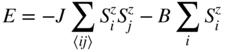
This feature is demonstrated in Figure 11.2, which in the main panel (full gray-shaded bins) reports the frequency of declarations obtained in the tax compliance experiment of Bazart and Bonein (2014). This experiment was designed as a pure declaration game, excluding redistribution of tax through the provision of public goods, and aimed to investigate reciprocal relationships in tax compliance decisions under various types of inequities. In each round (period) participants received an income of 100 points and were subject to certain fiscal policy parameters (e.g., tax audit, penalty rates, etc.; for details see Bazart and Bonein, 2014). Data shown in Figure 11.2 were obtained from the so-called horizontal inequity treatment where, at the end of each tax relevant period, participants learned the average income reported by the other members of their group. Important in the present context is that the declarations ![]() of most participants are close to either
of most participants are close to either ![]() or
or ![]() , which results in the bimodal distribution shown with the full bins in the main panel of Figure 11.2. In order to map this distribution to Ising data
, which results in the bimodal distribution shown with the full bins in the main panel of Figure 11.2. In order to map this distribution to Ising data ![]() one can introduce a threshold
one can introduce a threshold ![]() and assign all declarations with
and assign all declarations with ![]() to
to ![]() and all declarations with
and all declarations with ![]() to
to ![]() . In the Ising model, a participant with
. In the Ising model, a participant with ![]() is then represented by a spin
is then represented by a spin ![]() (i.e., a noncompliant agent) and a participant with
(i.e., a noncompliant agent) and a participant with ![]() corresponds to a compliant agent with
corresponds to a compliant agent with ![]() . Fixing the threshold to
. Fixing the threshold to ![]() yields the distribution shown by open bins in Figure 11.2 and one finds that the average of the experimental and Ising data is almost the same in each period of the experiment as shown in the inset to Figure 11.2. This agreement also supports the validity of an Ising description of tax evasion behavior.
yields the distribution shown by open bins in Figure 11.2 and one finds that the average of the experimental and Ising data is almost the same in each period of the experiment as shown in the inset to Figure 11.2. This agreement also supports the validity of an Ising description of tax evasion behavior.
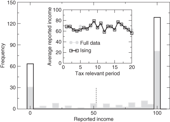
Figure 11.2 Main panel: The range of reported income  is divided into
  bins and the height of each bin corresponds to the frequency of declarations within the corresponding
  -interval. The Ising distribution (open bins) is obtained by assigning all declarations with
  to
to  and all declarations with
  to
to  . Inset: Upon setting
  (indicated by the dashed line) the Ising data give an excellent approximation to the average reported income as obtained from the experimental data (Bazart and Bonein, 2014) for all periods of the experiment.
Source: Figure reproduced from Bazart et al. 2016 by courtesy of the Journal of Tax Administration.
The horizontal inequity setting in the experiments of Bazart and Bonein (2014) aimed to study the question whether the evasion decision of one taxpayer will be conditional on those of all other taxpayers (see also Schnellenbach, 2010, and references therein). In fact, it was shown that some taxpayers did change their declaration decisions in the next period to get closer to the average reported income of other group members, that is, taxpayers tend to “copy” the predominant compliance behavior of those in their social network. In order to model this kind of behavior one has to take the interaction between agents into account, which in the Eq. (11.1) is due to the exchange constant ![]() . As illustrated in Figure 11.3 this interaction causes an agent to copy the average behavior of its “social network,” which for the simple structure depicted in Figure 11.3 consists of the four nearest neighbors but can be generalized in a straightforward manner to more complex networks.
. As illustrated in Figure 11.3 this interaction causes an agent to copy the average behavior of its “social network,” which for the simple structure depicted in Figure 11.3 consists of the four nearest neighbors but can be generalized in a straightforward manner to more complex networks.
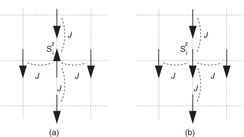
Figure 11.3 Social network of a tax payer on lattice site  for a square lattice with nearest-neighbor interactions. Shown are the situations of a honest (
 , (a)) and cheating (
 , (b)) agent, respectively, connected to noncompliant neighbors
In Figure 11.3(a) a honest tax payer (![]() ) interacts with noncompliant neighbors and, for the moment, we ignore the influence of an external field
) interacts with noncompliant neighbors and, for the moment, we ignore the influence of an external field ![]() . Within the Glauber dynamics, discussed earlier, a spin flip
. Within the Glauber dynamics, discussed earlier, a spin flip ![]() would then lower the energy by
would then lower the energy by ![]() (
(![]() per bond) so that the associated transition probability Eq. (11.7) is large at low temperature (i.e., for
per bond) so that the associated transition probability Eq. (11.7) is large at low temperature (i.e., for ![]() ). On the other hand, if the agent has the same evading behavior than its neighbors (Figure 11.3(b)) the energy change for the spin flip transition
). On the other hand, if the agent has the same evading behavior than its neighbors (Figure 11.3(b)) the energy change for the spin flip transition ![]() is positive (
is positive (![]() ) corresponding to a small transition probability at low temperature. In other words, the central agent tends to conform to the behavior of its neighbors where the adaptation increases with decreasing temperature. The latter parameter therefore is interpreted in Zaklan et al. (2008, 2009), Lima and Zaklan (2008) as a “social temperature parameter.” In Section 11.5 we will show that in the framework of discrete choice models this parameter can also be related to the fluctuations of unobserved utility. In their numerical modeling of tax evasion dynamics, Zaklan et al. associated a tax relevant period with an adjustment of all lattice spins based on the Glauber probability Eq. (11.7). Moreover, they introduced the probability of an efficient audit which means that the detection of tax evasion (i.e.,
) corresponding to a small transition probability at low temperature. In other words, the central agent tends to conform to the behavior of its neighbors where the adaptation increases with decreasing temperature. The latter parameter therefore is interpreted in Zaklan et al. (2008, 2009), Lima and Zaklan (2008) as a “social temperature parameter.” In Section 11.5 we will show that in the framework of discrete choice models this parameter can also be related to the fluctuations of unobserved utility. In their numerical modeling of tax evasion dynamics, Zaklan et al. associated a tax relevant period with an adjustment of all lattice spins based on the Glauber probability Eq. (11.7). Moreover, they introduced the probability of an efficient audit which means that the detection of tax evasion (i.e., ![]() ) forces the agent to stay honest over the following
) forces the agent to stay honest over the following ![]() time periods.
time periods.

Figure 11.4 Tax evasion dynamics on a  square lattice with nearest-neighbor interactions
  . (a, b) Results for agents with a social temperature of
  and audit probabilities
  and
and  , respectively. (c, d) The corresponding results for a social temperature of
  . The scale of temperature is set by
  . Tax audits enforce compliance over
  time steps. Initial condition is full compliance for all agents (
 ) except for (a) where the dashed line corresponds to an initial condition with full evasion (
 )
)
Figure 11.4 shows examples for the tax evasion dynamics obtained for selected parameter values on a ![]() square lattice with nearest-neighbor interactions. Since only the ratio
square lattice with nearest-neighbor interactions. Since only the ratio ![]() enters into the Glauber dynamics Eq. (11.7), the individual temperatures are specified with respect to
enters into the Glauber dynamics Eq. (11.7), the individual temperatures are specified with respect to ![]() . Figure 11.4(a) and (b) display the extent of tax evasion (i.e., the fraction of
. Figure 11.4(a) and (b) display the extent of tax evasion (i.e., the fraction of ![]() -spins) as a function of time for small “social temperature”
-spins) as a function of time for small “social temperature” ![]() and for small and large audit probabilities
and for small and large audit probabilities ![]() and
and ![]() , respectively. The initial condition is full compliance for all agents.3 Due to the small
, respectively. The initial condition is full compliance for all agents.3 Due to the small ![]() -value between the economics and econophysics based approach only a small number of agents become noncompliant in the first time step and because the audit probability is also small (Figure 11.4(a)), tax evasion
-value between the economics and econophysics based approach only a small number of agents become noncompliant in the first time step and because the audit probability is also small (Figure 11.4(a)), tax evasion ![]() increases continuously up to some saturation value
increases continuously up to some saturation value ![]() . At this value the system of agents has reached equilibrium between the influence of the neighborhood to become a noncompliant taxpayer and the tax audits which enforce compliance over
. At this value the system of agents has reached equilibrium between the influence of the neighborhood to become a noncompliant taxpayer and the tax audits which enforce compliance over ![]() time periods. Upon increasing the audit probability to
time periods. Upon increasing the audit probability to ![]() (Figure 11.4(b)) the number of tax evaders reaches its maximum already after about three time steps and then starts to decrease due to the high audit probability. After 10 time steps, initially detected tax evaders may again switch from compliant to noncompliant behavior, which leads to the observed small increase of
(Figure 11.4(b)) the number of tax evaders reaches its maximum already after about three time steps and then starts to decrease due to the high audit probability. After 10 time steps, initially detected tax evaders may again switch from compliant to noncompliant behavior, which leads to the observed small increase of ![]() before it reaches its saturation value of
before it reaches its saturation value of ![]() . Note that the “social temperature”
. Note that the “social temperature” ![]() is below the ordering temperature
is below the ordering temperature ![]() of the two-dimensional Ising model. For zero audit probability, the long-term tax evasion would therefore also converge to a small value (
of the two-dimensional Ising model. For zero audit probability, the long-term tax evasion would therefore also converge to a small value (![]() ), corresponding to the fraction of “minority spins” at this particular temperature. The effect of a finite audit probability is, therefore, just a further reduction from this small value.
), corresponding to the fraction of “minority spins” at this particular temperature. The effect of a finite audit probability is, therefore, just a further reduction from this small value.
In contrast, much above the ordering temperature the zero audit equilibrium state is reached for an equal number of compliant and noncompliant tax payers, that is, ![]() . Finite audit probabilities then lead to a further reduction of this equilibrium value. This situation is depicted in Figure 11.4(c) and (d), which display the extent of tax evasion for a system build up from agents who decide mainly autonomously, due to the large “social temperature”
. Finite audit probabilities then lead to a further reduction of this equilibrium value. This situation is depicted in Figure 11.4(c) and (d), which display the extent of tax evasion for a system build up from agents who decide mainly autonomously, due to the large “social temperature” ![]() (i.e., much larger than the exchange energy). As a consequence, already after two time steps approximately half of the agents become noncompliant, which in turn induces a reduction of
(i.e., much larger than the exchange energy). As a consequence, already after two time steps approximately half of the agents become noncompliant, which in turn induces a reduction of ![]() due to the auditing. It is remarkable that even for small audit probability
due to the auditing. It is remarkable that even for small audit probability ![]() (Figure 11.4(c))
(Figure 11.4(c)) ![]() decreases by
decreases by ![]() before it saturates at
before it saturates at ![]() after more than 10 time steps. Upon invoking a larger audit probability,
after more than 10 time steps. Upon invoking a larger audit probability, ![]() , the number of autonomous agents decreases rapidly after the first initial time steps and consequently
, the number of autonomous agents decreases rapidly after the first initial time steps and consequently ![]() decreases to almost zero within the first 10 time steps. Half the fraction of those who have been detected at the first time step will then select the possibility of noncompliance again, which leads to the oscillatory behavior of
decreases to almost zero within the first 10 time steps. Half the fraction of those who have been detected at the first time step will then select the possibility of noncompliance again, which leads to the oscillatory behavior of ![]() . A stable situation is only reached at
. A stable situation is only reached at ![]() time steps at
time steps at ![]() .
.
A more detailed discussion of related results can be found in Zaklan et al. (2008, 2009), and Lima and Zaklan (2008). In particular, the influence of a homogeneous magnetic field ![]() , interpreted as the influence of mass media, has been investigated by Lima and Zaklan (2008). In this context, a positive
, interpreted as the influence of mass media, has been investigated by Lima and Zaklan (2008). In this context, a positive ![]() would enhance the confidence in tax authorities whereas
would enhance the confidence in tax authorities whereas ![]() would imply a reduction of tax payers trust in governmental institutions. It has also been shown that the results are not sensitive to the specific lattice geometry. This issue has been analyzed in Zaklan et al. (2008, 2009), Lima and Zaklan (2008) where, in addition, alternative lattice structures such as the scale-free Barabási-Albert network or the Voronoi–Delaunay network have been considered. In addition, Lima (2010) investigates Erdös–Rényi random graphs and finds that the results for these alternative lattices do not differ significantly from those obtained with a square lattice. More recently, a generalization of the model with regard to the incorporation of nonequilibrium dynamics has been proposed in Lima (2010, 2012a,b).
would imply a reduction of tax payers trust in governmental institutions. It has also been shown that the results are not sensitive to the specific lattice geometry. This issue has been analyzed in Zaklan et al. (2008, 2009), Lima and Zaklan (2008) where, in addition, alternative lattice structures such as the scale-free Barabási-Albert network or the Voronoi–Delaunay network have been considered. In addition, Lima (2010) investigates Erdös–Rényi random graphs and finds that the results for these alternative lattices do not differ significantly from those obtained with a square lattice. More recently, a generalization of the model with regard to the incorporation of nonequilibrium dynamics has been proposed in Lima (2010, 2012a,b).
Extensions of the model concern also the implementation of different audit schemes. The original proposal (Zaklan et al., 2009, 2008) with enforcement of compliance over a fixed number of time steps upon detection of tax evasion has been investigated in a randomized variant in Lima and Zaklan (2008). Moreover, also lapse of time effects have been studied (Seibold and Pickhardt, 2013), that is, the situation where a detected agent is screened over several years in the past by the (tax) authorities (i.e., backaudit).
11.4 Heterogeneous Agents
In the original Zaklan model (Zaklan et al., 2008, 2009), each agent is either compliant or noncompliant and transitions between both behaviors are possible. However, the behavioral dynamics is governed by the Glauber probabilities (Eq. (11.7)) which, besides the contribution of the social network, depends on the “global parameters” temperature and magnetic field only. Therefore, agents in a social network consisting of the same number of cheating as well as honest tax payers have the same Glauber probabilities, which means that they are not endogenously different. However, most economic agent-based models assume behaviorally different agent types as, for instance, in the work of Hokamp and Pickhardt (2010) where four behavioral types have been introduced. First, they consider maximizing A-Types that show rational and risk-adverse behavior by maximizing their expected utility in agreement with Allingham and Sandmo (1972). Second, the model incorporates imitating B-Type agents that copy the behavior of the majority of their social network; that is, their decision on being compliant or noncompliant in the tax relevant period ![]() is dependent on the average compliance of agents in their social network at the previous period
is dependent on the average compliance of agents in their social network at the previous period ![]() . The third type of agents are “ethical” ones which, motivated by behavioral norms, are mostly compliant. Finally, random D-Types constitute the fourth type of agents. Due to the complexity of the tax law these agents may make unintended mistakes with respect to declaring their true income. Therefore, D-Types randomly switch between being compliant and noncompliant.
. The third type of agents are “ethical” ones which, motivated by behavioral norms, are mostly compliant. Finally, random D-Types constitute the fourth type of agents. Due to the complexity of the tax law these agents may make unintended mistakes with respect to declaring their true income. Therefore, D-Types randomly switch between being compliant and noncompliant.
How can we implement these behaviorally different agents into the Ising model description of tax evasion discussed in Section 11.3. Concerning the A-Type agents it is obviously not possible to have risk-adverse behavior in our ecophysics model. Within the approach of Allingham and Sandmo (1972) this would imply a concave utility function which allows for an “inner solution,” that is, the possibility that agents declare part of their income. However, the variables in the Ising model can take only two values, ![]() corresponding to full- or zero-income declaration. In the Allingham–Sandmo model, such agents are risk-neutral with an utility function which is linear in the after tax and penalty net income. This yields full (zero) declaration if the audit probability
corresponding to full- or zero-income declaration. In the Allingham–Sandmo model, such agents are risk-neutral with an utility function which is linear in the after tax and penalty net income. This yields full (zero) declaration if the audit probability ![]() is larger (smaller) than the ratio between the tax rates of declared and undeclared income. In practice this means that for real values of the various parameters risk-neutral A-Type agents mostly declare zero income. In the Ising model we can implement such behavior by coupling the spin that represents the A-Type to a local negative magnetic field
is larger (smaller) than the ratio between the tax rates of declared and undeclared income. In practice this means that for real values of the various parameters risk-neutral A-Type agents mostly declare zero income. In the Ising model we can implement such behavior by coupling the spin that represents the A-Type to a local negative magnetic field ![]() , that is, the energy functional equation (11.1) is supplemented by a term
, that is, the energy functional equation (11.1) is supplemented by a term

where the summation runs over all sites that are occupied by an A-Type. Inspection of the Glauber probability equation (11.7) reveals that the magnetic field has only a significant influence when it is (i) larger than the contribution from neighbors (i.e., ![]() ) and (ii) when it is not overcome by large temperature fluctuations. In order to locally satisfy the last criterion we couple each site
) and (ii) when it is not overcome by large temperature fluctuations. In order to locally satisfy the last criterion we couple each site ![]() to a heat bath with temperature
to a heat bath with temperature ![]() , that is, in contrast to the original Zaklan model (Zaklan et al., 2008, 2009) temperature is not a global parameter but is locally defined at each site.4 For A-Types this means that in addition
, that is, in contrast to the original Zaklan model (Zaklan et al., 2008, 2009) temperature is not a global parameter but is locally defined at each site.4 For A-Types this means that in addition ![]() should be satisfied in order to obtain large Glauber probabilities for
should be satisfied in order to obtain large Glauber probabilities for ![]() states on the A-Type sites. In the same way, C-Type agents can be modeled by the coupling to local magnetic fields
states on the A-Type sites. In the same way, C-Type agents can be modeled by the coupling to local magnetic fields ![]() via
via

where again the relations ![]() and
and ![]() should be satisfied in order to have the dominant influence on the Glauber probabilities given by
should be satisfied in order to have the dominant influence on the Glauber probabilities given by ![]() . The positive sign of the field (as opposed to the negative A-Type field
. The positive sign of the field (as opposed to the negative A-Type field ![]() ) lowers the energy contribution Eq. (11.9) for
) lowers the energy contribution Eq. (11.9) for ![]() states.
states.
For imitating B-Type agents the Glauber probability should be maximized for spin states close to the average spin of their social network. For this purpose we model these agents by a small local temperature ![]() so that the influence of the interaction energy
so that the influence of the interaction energy ![]() is dominant. Also, random D-Types are characterized by the local temperature, which has to satisfy
is dominant. Also, random D-Types are characterized by the local temperature, which has to satisfy ![]() . In this case, one sees from Eq. (11.7) that the Glauber probabilities are close to
. In this case, one sees from Eq. (11.7) that the Glauber probabilities are close to ![]() , that is, the random agent is strongly fluctuating between compliant and noncompliant behavior.
, that is, the random agent is strongly fluctuating between compliant and noncompliant behavior.

Figure 11.5 Ising model with heterogeneous agent types. Each site is coupled to a heat bath with temperature  as indicated by boxes. Moreover, A-Type agents are coupled to a negative magnetic field (e.g., site
  ) whereas C-Type agents are coupled to a positive magnetic field (e.g., site
  ). Nearest neighbors are coupled by the exchange constant
Figure 11.5 illustrates the Ising model design for heterogeneous agents for a ![]() lattice with nearest-neighbor couplings
lattice with nearest-neighbor couplings ![]() . Every site is coupled to an individual heat bath with temperature
. Every site is coupled to an individual heat bath with temperature ![]() , represented by the boxes. Moreover, the spins on A-Type (C-Type) sites are coupled to a negative (positive) magnetic field (as visualized by the large gray arrow). The parameter ranges for the individual agent types are summarized in Table 11.1.
, represented by the boxes. Moreover, the spins on A-Type (C-Type) sites are coupled to a negative (positive) magnetic field (as visualized by the large gray arrow). The parameter ranges for the individual agent types are summarized in Table 11.1.
Clearly, the various agent types are textbook cases for the individual behavior of tax payers. In principle, one can parametrize an agent at lattice site ![]() by an arbitrary combination for the field and temperature values
by an arbitrary combination for the field and temperature values ![]() ,
, ![]() so that besides the “pure” types, also agents with an intermediate behavior (e.g., between A- and B-Types) are possible. In fact, this is what one finds when the parameters are calibrated with tax compliance laboratory experiments (Bazart et al., 2016).
so that besides the “pure” types, also agents with an intermediate behavior (e.g., between A- and B-Types) are possible. In fact, this is what one finds when the parameters are calibrated with tax compliance laboratory experiments (Bazart et al., 2016).
Table 11.1 Summary of parameter ranges that specify the various agent types in the heterogeneous Ising model
| Type | Parameter specification |
| a | |
| b | |
| c | |
| d |
Figure 11.6 shows the Glauber probabilities (Eq. (11.7)) for a compliant tax payer switching to noncompliance in the ![]() parameter space. Figure 11.6(a) (Figure 11.6(b)) reports the situation that all neighbors are noncompliant (compliant) and the “pure” agent-types are indicated in the panels. For example, a compliant A-Type (which can be the result of an audit) has always probability
parameter space. Figure 11.6(a) (Figure 11.6(b)) reports the situation that all neighbors are noncompliant (compliant) and the “pure” agent-types are indicated in the panels. For example, a compliant A-Type (which can be the result of an audit) has always probability ![]() to switch to noncompliance, irrespective of the behavior of neighbors. It is also apparent from Figure 11.6 that only the probability of B-Types strongly depends on the state of the nearest neighbors. In any case, it is possible to change the behavior of agents continuously by changing the field and (or) temperature parameters and therefore to have agents with an intermediate behavior between the “pure” types.
to switch to noncompliance, irrespective of the behavior of neighbors. It is also apparent from Figure 11.6 that only the probability of B-Types strongly depends on the state of the nearest neighbors. In any case, it is possible to change the behavior of agents continuously by changing the field and (or) temperature parameters and therefore to have agents with an intermediate behavior between the “pure” types.

Figure 11.6 Field-temperature parameter space of probabilities for the transition of an agent from compliance to noncompliance. (a) All nearest neighbors are compliant ( ), (b) All nearest neighbors are noncompliant (
 ) as illustrated in Figure 11.3.
  -field values are in units of the exchange constant
  whereas temperature
  values are given in units of

Figure 11.7 Tax evasion dynamics for the multi-agent Ising model. In each panel the percentage of two agent-types is fixed to  as indicated in the heading. The fraction of the other two agent-types is then varied in steps of
  . System size:
  square lattice with nearest-neighbor coupling
  . Enforced compliance period after audit:
  time steps. Agents are specified by the following parameters: A-Types (
 ,
,  ), B-Types (
 ,
,  ), C-Types (
 ,
,  ), D-Types (
 ,
,  ). Temperature values are in units of
  and field values in units of
Figure 11.7 reports the tax evasion dynamics (i.e., the fraction of ![]() agents) for different compositions of the heterogeneous tax payer society. For simplicity we restrict to “pure” agent-types with the corresponding parameter values given in the caption to Figure 11.7. Initial conditions at time step
agents) for different compositions of the heterogeneous tax payer society. For simplicity we restrict to “pure” agent-types with the corresponding parameter values given in the caption to Figure 11.7. Initial conditions at time step ![]() are such that
are such that ![]() for C-Types and
for C-Types and ![]() for A-, B-, and D-Type agents. As shown in Figure 11.4 the equilibrium value at large times does not depend on these initial conditions as these are only relevant on a short time scale after
for A-, B-, and D-Type agents. As shown in Figure 11.4 the equilibrium value at large times does not depend on these initial conditions as these are only relevant on a short time scale after ![]() . For this reason, the initial fraction of tax evasion in Figure 11.7 is always one minus the fraction of C-Types. Panel I.) of Figure 11.7 shows the evasion dynamics for
. For this reason, the initial fraction of tax evasion in Figure 11.7 is always one minus the fraction of C-Types. Panel I.) of Figure 11.7 shows the evasion dynamics for ![]() B- and D-Types, while the respective fraction of noncompliant A-Types and fully compliant C-Types varies by
B- and D-Types, while the respective fraction of noncompliant A-Types and fully compliant C-Types varies by ![]() . This also induces a variation in the long-term tax evasion of about
. This also induces a variation in the long-term tax evasion of about ![]() , which is slightly larger because of the contribution of B-Types that copy the behavior of A- and C-Types when they are nearest neighbors. In panel II.) the percentage of A- and C-Types is fixed to
, which is slightly larger because of the contribution of B-Types that copy the behavior of A- and C-Types when they are nearest neighbors. In panel II.) the percentage of A- and C-Types is fixed to ![]() whereas the relative fraction of B- and D-Types is varied. Note that an ensemble of B-Types is predominantly compliant (cf. Figure 11.4(a, b)) whereas the tax evasion of random D-Types approaches 0.5 for low audit rates (cf. Figure 11.4(c)). Therefore, a shift of the relative fraction from B- to D-Types, as in panel II.), increases tax evasion, where the increment decreases with decreasing percentage of B-Types. This is due to the decreasing amount of B-Type clusters that contribute to compliance so that for smaller fractions of B-Types these are predominantly connected to A- and C-Types. The corresponding imitating effect compensates and therefore tax evasion increases by a lesser degree when the fraction of B-Types is reduced from
whereas the relative fraction of B- and D-Types is varied. Note that an ensemble of B-Types is predominantly compliant (cf. Figure 11.4(a, b)) whereas the tax evasion of random D-Types approaches 0.5 for low audit rates (cf. Figure 11.4(c)). Therefore, a shift of the relative fraction from B- to D-Types, as in panel II.), increases tax evasion, where the increment decreases with decreasing percentage of B-Types. This is due to the decreasing amount of B-Type clusters that contribute to compliance so that for smaller fractions of B-Types these are predominantly connected to A- and C-Types. The corresponding imitating effect compensates and therefore tax evasion increases by a lesser degree when the fraction of B-Types is reduced from ![]() to
to ![]() as compared to the reduction from
as compared to the reduction from ![]() to
to ![]() (with a corresponding increase in the fraction of D-Types). The situation of fixed percentages (
(with a corresponding increase in the fraction of D-Types). The situation of fixed percentages (![]() ) for A- and D-Types is illustrated in panel III.). For an additional fraction of
) for A- and D-Types is illustrated in panel III.). For an additional fraction of ![]() for B-Types, the long-term tax evasion is
for B-Types, the long-term tax evasion is ![]() , that is, about 0.25 points larger than what one expects from the contribution of A- (
, that is, about 0.25 points larger than what one expects from the contribution of A- (![]() ) and D- (
) and D- (![]() ) types. Clearly, this “excess” evasion comes from the imitating B-Types, which, due to the interaction with noncompliant A-Types, contribute to tax evasion. Decreasing the fraction of B-Types with a similar increase of C-Types obviously enhances compliance because now the still significant fraction of B-Types (cf. e.g., the result for
) types. Clearly, this “excess” evasion comes from the imitating B-Types, which, due to the interaction with noncompliant A-Types, contribute to tax evasion. Decreasing the fraction of B-Types with a similar increase of C-Types obviously enhances compliance because now the still significant fraction of B-Types (cf. e.g., the result for ![]() B-Types) can also imitate the compliant C-Type behavior. This effect vanishes for a small percentage of B-Types so that in this limit panel III.) only shows a weak variation of the corresponding long-term evasion. Finally, panel IV.) shows the result for fixed C- and D-Type fraction while the percentage of A- and C-Types is changed. Here the increase of A-Types naturally increases evasion with a larger increment for small A-Type fractions panel III.).This is due to the effect of B-Types that now imitate the A-Types whereas this effect obviously vanishes for small fractions of B-Types.
B-Types) can also imitate the compliant C-Type behavior. This effect vanishes for a small percentage of B-Types so that in this limit panel III.) only shows a weak variation of the corresponding long-term evasion. Finally, panel IV.) shows the result for fixed C- and D-Type fraction while the percentage of A- and C-Types is changed. Here the increase of A-Types naturally increases evasion with a larger increment for small A-Type fractions panel III.).This is due to the effect of B-Types that now imitate the A-Types whereas this effect obviously vanishes for small fractions of B-Types.
The key issue for calculating the tax evasion dynamics within the heterogeneous Ising model is certainly to get reasonable estimates for the fraction of the different agent types. A first step in this direction has been undertaken by Hokamp and Seibold (2014) in the analysis of the shadow economies in France and Germany within a similar model. Here, the results from laboratory experiments on tax compliance (Bazart and Pickhardt, 2011) have been used to extract the full compliance ratio (i.e., essentially the fraction of C-Types) of ![]() and
and ![]() for Germany and France, respectively. Note that the compliance ratio only specifies the percentage of subjects which showed fully compliant behavior in each round of the experiment. The average compliance rate which determines tax evasion is larger. Since no data are available for the percentage of D-Type agents the corresponding number was taken from Andreoni et al. (1998) which reports that about 7% of US households overpaid their taxes in 1988. If one anticipates that about the same amount of people underpays their taxes one arrives at a percentage of
for Germany and France, respectively. Note that the compliance ratio only specifies the percentage of subjects which showed fully compliant behavior in each round of the experiment. The average compliance rate which determines tax evasion is larger. Since no data are available for the percentage of D-Type agents the corresponding number was taken from Andreoni et al. (1998) which reports that about 7% of US households overpaid their taxes in 1988. If one anticipates that about the same amount of people underpays their taxes one arrives at a percentage of ![]() of D-Type agents (cf. also Hokamp and Pickhardt, 2010). Hokamp and Seibold (2014) then determine the fraction of A- and B-Type agents that participate in the shadow economy in France and Germany, respectively. Calculations were performed for the two audit schemes with fixed compliance period and backaudit where for the latter a backaudit period of
of D-Type agents (cf. also Hokamp and Pickhardt, 2010). Hokamp and Seibold (2014) then determine the fraction of A- and B-Type agents that participate in the shadow economy in France and Germany, respectively. Calculations were performed for the two audit schemes with fixed compliance period and backaudit where for the latter a backaudit period of ![]() time steps has been considered. The latter is compatible with the limitation period of five years in
time steps has been considered. The latter is compatible with the limitation period of five years in ![]() where the experiments by Bazart and Pickhardt (2011) have been conducted. Data on the shadow economies for France and Germany were adopted from Buehn and Schneider (2012), which for the two countries reports
where the experiments by Bazart and Pickhardt (2011) have been conducted. Data on the shadow economies for France and Germany were adopted from Buehn and Schneider (2012), which for the two countries reports ![]() and
and ![]() of the official GDP, respectively, averaged over the period 1999–2007. These numbers are supported by the data of Elgin and Öztunali (2012), which report
of the official GDP, respectively, averaged over the period 1999–2007. These numbers are supported by the data of Elgin and Öztunali (2012), which report ![]() for OECD EU-countries in the period from 2001–2009. As a result, the analysis revealed a larger share of A-Type agents for Germany, where the absolute magnitude and the difference to France depends on the considered enforcement scheme. For example, the back audit mechanism results in a fraction of
for OECD EU-countries in the period from 2001–2009. As a result, the analysis revealed a larger share of A-Type agents for Germany, where the absolute magnitude and the difference to France depends on the considered enforcement scheme. For example, the back audit mechanism results in a fraction of ![]() A-Types for France and
A-Types for France and ![]() A-Types for Germany. The missing fraction then corresponds to the B-Types, which yields
A-Types for Germany. The missing fraction then corresponds to the B-Types, which yields ![]() (Germany) and
(Germany) and ![]() (France). Note that a more direct estimate for the percentage of agent types has been performed recently in Bazart et al. (2016) where the field and temperature parameter has been determined for individual participants in a tax evasion laboratory experiment.
(France). Note that a more direct estimate for the percentage of agent types has been performed recently in Bazart et al. (2016) where the field and temperature parameter has been determined for individual participants in a tax evasion laboratory experiment.
11.5 Relation to Binary Choice Model
There is a close relationship between the Glauber probabilities in Eq. (11.7) and the probabilities which can be derived within the logit discrete choice model. The development of the latter was awarded with the 2000 Nobel prize in economics to Daniel L. McFadden “for his development of theory and methods for analyzing discrete choice.” This connection therefore allows to link the dynamics of the behavioral dynamics obtained from utility-maximizing behavior and therefore provides a link between econophysics and classical economics description of tax evasion.
Consider an agent, in the present context called decision maker, which can choose between the two alternatives of declaring zero or full income. Taking again an ensemble of heterogeneous agents, the decision maker n obtains a certain level of utility (or profit) from each alternative, which we denote by ![]() with
with ![]() corresponding to zero and full income declaration, respectively. Further on we assume that the individual's utility from choosing the alternative j takes the form
corresponding to zero and full income declaration, respectively. Further on we assume that the individual's utility from choosing the alternative j takes the form ![]() , where
, where ![]() is common to all individuals with observed attributes j (i.e., declaration of full or zero income), while
is common to all individuals with observed attributes j (i.e., declaration of full or zero income), while ![]() is particular to the drawn individual. Both utility terms are deterministic, the first reflecting “representative” (and observable) tastes in the population, and the second reflecting (unobservable) idiosyncratic taste variations. The probability
is particular to the drawn individual. Both utility terms are deterministic, the first reflecting “representative” (and observable) tastes in the population, and the second reflecting (unobservable) idiosyncratic taste variations. The probability ![]() that decision maker
that decision maker ![]() chooses alternative
chooses alternative ![]() is then given by
is then given by

and the probabilities are normalized, ![]() .
.
The basic assumption of the logit model is that the unobserved contributions, ![]() , are independent with regard to agent
, are independent with regard to agent ![]() , and alternative
, and alternative ![]() and are specified by the Gumbel or double exponential probability density
and are specified by the Gumbel or double exponential probability density
The probabilities equation (11.10) can therefore be expressed via the corresponding cumulative distribution
weighted by the density of the unknown ![]() . One finds for the probability of zero income declaration for agent
. One finds for the probability of zero income declaration for agent ![]()

where the integration can be easily performed by substituting ![]() . Similarly, the probability for full income declaration is obtained as
. Similarly, the probability for full income declaration is obtained as
so that the condition ![]() is satisfied. Thus the decision probability on declaring zero or full income depends on the difference between the corresponding observable parts of the utility function
is satisfied. Thus the decision probability on declaring zero or full income depends on the difference between the corresponding observable parts of the utility function ![]() . In case
. In case ![]() , which yields
, which yields ![]() , the agent will most probably declare zero income while full income declaration is most probable for
, the agent will most probably declare zero income while full income declaration is most probable for ![]() . From Eq. (11.10) it turns out that the decision probabilities are solely determined by utility differences so that the utility functions themselves are only specified up to a constant. Moreover, since the agent chooses the alternative with the largest utility the overall scale of the utility function does not influence on the decision. One possibility (Train, 2002) to normalize the scale of utility is to fix the variance of the unobserved contributions
. From Eq. (11.10) it turns out that the decision probabilities are solely determined by utility differences so that the utility functions themselves are only specified up to a constant. Moreover, since the agent chooses the alternative with the largest utility the overall scale of the utility function does not influence on the decision. One possibility (Train, 2002) to normalize the scale of utility is to fix the variance of the unobserved contributions ![]() , that is, to scale the utility by a factor
, that is, to scale the utility by a factor ![]() such that
such that  . Note that we consider here the possibility that the variance
 ![]() (or the “range of taste variations”) is different among agents. For each agent the rescaled utility functions
(or the “range of taste variations”) is different among agents. For each agent the rescaled utility functions ![]() has then the property
has then the property ![]() and one finds for the corresponding probabilities of zero and full income declaration
and one finds for the corresponding probabilities of zero and full income declaration
For each agent the probabilities are therefore determined by the ratio between the observable utility parts and the standard deviation of the unobservable contribution. For independent (isolated) agents the difference between Eqs (11.13) and (11.14) and Eqs (11.15) and (11.16) is irrelevant since the relative order of probabilities is preserved under the rescaling. However, it matters if we consider interacting agents where the utility function of agent ![]() may also depend on the decisions of the neighbors in the network. The construction of such an utility function for interacting agents is facilitated by noting the similarity of Eqs (11.15) and (11.16) with the Glauber probability equation (11.7), which provides a correspondence between the difference in observable utility divided by the standard deviation of unobserved utility and the energy difference in the Ising model divided by (local) temperature
may also depend on the decisions of the neighbors in the network. The construction of such an utility function for interacting agents is facilitated by noting the similarity of Eqs (11.15) and (11.16) with the Glauber probability equation (11.7), which provides a correspondence between the difference in observable utility divided by the standard deviation of unobserved utility and the energy difference in the Ising model divided by (local) temperature
In particular, this also suggests a correspondence between the observable part of the utility function and the (negative) energy in the Ising model which is reasonable since a state with lower energy (i.e., more negative) has larger probability in the Monte-Carlo dynamics and therefore larger utility from the perspective of a discrete choice model. Moreover, the correspondence (Eq.(11.17)) offers an interpretation of temperature in terms of the standard deviation of the unobservable utility part. The latter refers to the spread in the nonmeasurable taste or attitude so that according to our previous classification noncompliant (A-Types), copying (B-Types), and compliant (C-Types) agents are characterized by a small ![]() corresponding to their fixed moral attitude towards tax evasion (A- and C-Types) or their fixed copying behavior (B-Types). On the other hand, random D-Types display large variations of attitude toward evasion and thus can be described by a large
corresponding to their fixed moral attitude towards tax evasion (A- and C-Types) or their fixed copying behavior (B-Types). On the other hand, random D-Types display large variations of attitude toward evasion and thus can be described by a large ![]() . Thus the standard deviation of the unobserved utility
. Thus the standard deviation of the unobserved utility ![]() specifies the agents in the same way than the temperature parameter
specifies the agents in the same way than the temperature parameter ![]() in the Ising model which was empirically fixed based on the functional form of the Glauber transition probabilities equation (11.7).
in the Ising model which was empirically fixed based on the functional form of the Glauber transition probabilities equation (11.7).
11.6 Summary and Outlook
Among the agent-based models for tax evasion discussed in this book, the Ising model-based approach may be considered as a “maverick” since it is not derived from an economic perspective but adopted from physics so that its validity in the present context at a first glance seems rather ill-founded. One issue concerns the fact that agents following the Ising model approach can only declare zero or full income. In this regard we have seen in Section 11.3 that a variety of data supports a bimodal distribution in the reported income compatible with an Ising-type behavior of taxpayers. In principle, the restriction of “two-state” Ising agents can be resolved by generalizing the description in terms of the so-called Potts model (Potts, 1952; Wu, 1982) where each spin (agent) can take ![]() orientations and the limit
orientations and the limit ![]() would then correspond to the standard Ising model. In this way it would be possible to discretize the taxable income into
would then correspond to the standard Ising model. In this way it would be possible to discretize the taxable income into ![]() bins and also to specify the reported income within these
bins and also to specify the reported income within these ![]() values. This would also allow to attribute to each agent an after tax and income whereas the present Ising model formulation only provides information about compliance decisions. A first step in this direction has been recently undertaken by Crokidakis (2014).
values. This would also allow to attribute to each agent an after tax and income whereas the present Ising model formulation only provides information about compliance decisions. A first step in this direction has been recently undertaken by Crokidakis (2014).
We have seen in Section 11.5 that one can derive a correspondence between the observable part of the utility function and the (negative) energy in the Ising model, which thus provides a link between the economics-based approach and the econophysics-based approach. This allows to study the differences between both descriptions with regard to the implementation of the dynamics and also the direct (nonmarket based) interaction among agents. Concerning the dynamical aspect, agent-based models from the economics domain are often based on a generalization of the Allingham–Sandmo theory (Allingham and Sandmo, 1972) where either all or a subgroup of agents display rational behavior (cf. e.g., Hokamp and Pickhardt, 2010 and references therein) so that there exists an utility function with is inhomogeneous with respect to the parameters specifying net income, perceived audit probability, and so on. The dynamics is then implemented by requiring at each time step ![]() (i.e., at each tax relevant period) the stationarity of the utility function. This means that rational agents decide instantaneously on their declared income
(i.e., at each tax relevant period) the stationarity of the utility function. This means that rational agents decide instantaneously on their declared income ![]() that only depends on the parameter values
that only depends on the parameter values ![]() in the same period. On the other hand, in the econophysics approach, the Ising model dynamics is governed by Glauber transition probabilities equation (11.7) [or equivalently Eqs (11.15) and (11.16)], which therefore corresponds to a Markov process.5 This means that also in this case the dynamics is “memoryless” with the difference that the state of the system at time step
in the same period. On the other hand, in the econophysics approach, the Ising model dynamics is governed by Glauber transition probabilities equation (11.7) [or equivalently Eqs (11.15) and (11.16)], which therefore corresponds to a Markov process.5 This means that also in this case the dynamics is “memoryless” with the difference that the state of the system at time step ![]() is solely determined by the state at time step
is solely determined by the state at time step ![]() . As a consequence the “econophysics dynamics” does not necessarily correspond to the saddle point of the utility function and also explores the fluctuating environment. Concerning the interactions among agents, the econophysics Ising model description includes these as nonlinearities of the spin variables in the energy functional (or utility function). The dynamics of imitating taxpayers is then obtained within the same Glauber formalism as for (non)compliant agents, which only differ by their parameter values (i.e., local temperature and field). On the other hand, economic agent-based models often use distinct dynamics for imitating agents as compared to rational ones. For example, Hokamp and Pickhardt (2010) evaluate the ratio of declared [
. As a consequence the “econophysics dynamics” does not necessarily correspond to the saddle point of the utility function and also explores the fluctuating environment. Concerning the interactions among agents, the econophysics Ising model description includes these as nonlinearities of the spin variables in the energy functional (or utility function). The dynamics of imitating taxpayers is then obtained within the same Glauber formalism as for (non)compliant agents, which only differ by their parameter values (i.e., local temperature and field). On the other hand, economic agent-based models often use distinct dynamics for imitating agents as compared to rational ones. For example, Hokamp and Pickhardt (2010) evaluate the ratio of declared [![]() ] and full [
] and full [![]() ] income of imitating B-Types at time step
] income of imitating B-Types at time step ![]() from the average ratio of the social network at the previous time step
from the average ratio of the social network at the previous time step ![]() , that is, contrary to rational agents the dynamics of B-Types is not instantaneous. Summarizing, the appealing feature of the Ising model-based econophysics approach to tax evasion is the coherent description of agent types within a minimal parameter set. The calibration of tax compliance experiments (Bazart et al., 2016) even reveals that it is possible to characterize the decision probability of participants with a temperature and field parameter, which offers a new perspective for the quantitative evaluation of such investigations. As discussed earlier a future generalization of the formalism can be achieved on the basis of the Potts model that allows for a more quantitative description of pay-offs and therefore of a more realistic implementation of audit schemes.
, that is, contrary to rational agents the dynamics of B-Types is not instantaneous. Summarizing, the appealing feature of the Ising model-based econophysics approach to tax evasion is the coherent description of agent types within a minimal parameter set. The calibration of tax compliance experiments (Bazart et al., 2016) even reveals that it is possible to characterize the decision probability of participants with a temperature and field parameter, which offers a new perspective for the quantitative evaluation of such investigations. As discussed earlier a future generalization of the formalism can be achieved on the basis of the Potts model that allows for a more quantitative description of pay-offs and therefore of a more realistic implementation of audit schemes.
References
- Agliari, E., Casartelli, M., and Vezzani, A. (2010) Microscopic energy flows in disordered Ising spin systems. Journal of Statistical Mechanics: Theory and Experiment, P10021-1–13.
- Allingham, M.G. and Sandmo, A. (1972) Income tax evasion: a theoretical analysis. Journal of Public Economics, 1, 323–338.
- Alm, J. and McKee, M. (2006) Audit certainty, audit productivity, and taxpayer compliance. National Tax Journal, 59, 801–816.
- Alm, J., Deskins, J., and McKee, M. (2009) Do individuals comply on income not reported by their employer? Public Finance Review, 37, 120–141.
- Andreoni, J., Erard, B., and Feinstein, J. (1998) Tax compliance. Journal of Economic Literature, 36, 818–860.
- Bazart, C. and Bonein, A. (2014) Reciprocal relationships in tax compliance decisions. Journal of Economic Psychology, 40, 83–102.
- Bazart, C., Bonein, A., Hokamp, S., and Seibold, G. (2016) Behavioral economics, tax evasion and the shadow economy – calibrating an agent-based econophysics model with experimental tax compliance data. Journal of Tax Administration, 2, 126–144.
- Bazart, C. and Pickhardt, M. (2011) Fighting income tax evasion with positive rewards. Public Finance Review, 39, 124–149.
- Binder, K. and Heermann, D.W. (2010) Monte Carlo Simulation in Statistical Physics, Springer-Verlag, Heidelberg, Dordrecht, London, New York.
- Bloomquist, K. (2011) Tax compliance as an evolutionary coordination game. Public Finance Review, 39, 25–49.
- Buehn, A. and Schneider, F. (2012) Shadow economies around the world: novel insights, accepted knowledge, and new estimates. International Tax and Public Finance, 19, 139–171.
- Castellano, C., Fortunato, S., and Loreto, V. (2009) Statistical physics of social dynamics. Reviews of Modern Physics, 81, 591–646.
- Chakraborti, A., Toke, I.M., Patriarca, M., and Abergel, F. (2011a) Econophysics review: I. Empirical facts. Quantitative Finance, 11, 991–1012.
- Chakraborti, A., Toke, I.M., Patriarca, M., and Abergel, F. (2011b) Econophysics review: II. Agent-based models. Quantitative Finance, 11, 1013–1041.
- Chen, S.-H. and Li, S.-P. (2012) Econophysics: bridges over a turbulent current. International Review of Finance Analysis, 23, 1–10.
- Crokidakis, N. (2014) A three-state kinetic agent-based model to analyze tax evasion dynamics. Physica A, 414, 321–328.
- Elgin, C. and Öztunali, O. (2012) Shadow economies around the world: model based estimates. Working Papers 2012/05, Bogazici University, Department of Economics.
- Föllmer, H. (1974) Random economies with many interacting agents. Journal of Mathematical Economics, 1, 51–62.
- Galam, S. (2012) Sociophysics, Springer-Verlag, Berlin.
- Gallegati, M., Keen, S., Lux, T., and Ormerod, P. (2006) Worrying trends in econophysics. Physica A, 370, 1–6.
- Harris, R. and Grant, M. (1988) Thermal conductivity of a kinetic Ising model. Physical Review B, 38, 9323–9326.
- Huang, K. (1987) Statistical Mechanics, John Wiley & Sons, Inc., New York.
- Hokamp, S. and Pickhardt, M. (2010) Income tax evasion in a society of heterogeneous agents - evidence from an agent-based model. International Economic Journal, 24, 541–553.
- Hokamp, S. and Seibold, G. (2014) How much rationality tolerates the shadow economy? An agent-based econophysics approach, in Advances in Social Simulation - Proceedings of the 9th Conference of the European Social Simulation Association (eds B. Kaminski and G. Koloch), Springer-Verlag, Berlin/Heidelberg, pp. 119–128.
- Ising, E. (1925) Beitrag zur Theorie des Ferromagnetismus. Zeitschrift fur Physik, 31, 253–258.
- Krauth, W. (2006) Statistical Mechanics; Algorithms and Computations, Oxford University Press.
- Lima, F.W.S. (2010) Analysing and controlling the tax evasion dynamics via majority-vote model. Journal of Physics: Conference Series, 246, 012033, 12 pp.
- Lima, F.W.S. (2012a) Three-state majority-vote model on square lattice. Physica A, 391, 1753–1758.
- Lima, F.W.S. (2012b) Tax evasion dynamics and Zaklan model on opinion-dependent network. International Journal of Modern Physics C, 23, 1250047–11.
- Lima, F.W.S. and Zaklan, G. (2008) A multi-agent-based approach to tax morale. International Journal of Modern Physics C, 19, 1797–1808.
- Liu, Y., Gopikrishnan, P., Cizeau, P. et al. (1999) Statistical properties of the volatility of price fluctuations. Physical Review E, 60, 1390–1400.
- Lux, T. and Marchesi, M. (1999) Scaling and criticality in a stochastic multi-agent model of a financial market. Nature, 397, 498–500.
- McCauley, J. (2004) Dynamics of Markets, Econophysics and Finance, Cambridge University Press.
- Mantegna, R.N. and Stanley, H.E. (2000) An Introduction to Econophysics - Correlations and Complexity in Finance, Cambridge University Press.
- Metropolis, N., Rosenbluth, A.W., Rosenbluth, M.N. et al. (1953) Equation of state calculations by fast computing machines. Journal of Chemical Physics, 21, 1087–1092.
- Onsager, L. (1944) Crystal statistics. I. A two-dimensional model with an order-disorder transition. Physical Review B, 65, 117–149.
- Patriarca, M., Chakraborti, A., and Kaski, K. (2004) Statistical model with a standard
 distribution. Physical Review E, 70, 016104-1–5.
 - Pickhardt, M. and Seibold, G. (2014) Income tax evasion dynamics: evidence from an agent-based econophysics model. Journal of Economic Psychology, 40, 147–160.
- Potts, R.B. (1952) Some generalized order-disorder transformations. Mathematical Proceedings of the Cambridge Philosophical Society, 48, 106–109.
- Schnellenbach, J. (2010) Vertical and horizontal reciprocity in a theory of taxpayer compliance, in Developing Alternative Frameworks for Explaining Tax Compliance (eds J. Alm, J. Martinez-Vasquez, and B. Torgler), Routledge International Studies in Money and Banking, Routledge, pp. 56–73.
- Seibold, G. and Pickhardt, M. (2013) Lapse of time effects on tax evasion in an agent-based econophysics model. Physica A, 392, 2079–2087.
- Sen, P. and Chakrabarti, B.K. (2013) Sociophysics: An Introduction, Oxford University Press.
- Sornette, D. (2014) Physics and financial economics (1776–2014): puzzles, Ising and agent-based models. Reports on Progress in Physics, 77, 062001-1–28.
- Stanley, M.H.R., Amaral, L.A.N., Buldyrev, S.V. et al. (1996) Scaling behaviour in the growth of companies. Nature, 379, 804–806.
- Stanley, H.E., Amaral, L.A.N., Gabaix, X. et al. (2001) Similarities and differences between physics and economics. Physica A, 299, 1–15.
- Train, K.E. (2002) Discrete Choice Methods with Simulation, Cambridge University Press.
- Uhlenbeck, G.E. and Goudsmit, S. (1925) Ersetzung der Hypothese vom unmechanischen Zwang durch eine Forderung bezüglich des inneren Verhaltens jedes einzelnen Elektrons. Naturwissenschaften, 47, 953–954.
- Wu, F.Y. (1982) The Potts model. Reviews of Modern Physics, 54, 235–268.
- Yamasaki, K., Muchnik, L., Havlin, S. et al. (2005) Scaling and memory in volatility return intervals in financial markets. Proceedings of the National Academy of Sciences of the United States of America, 102, 9424–9428.
- Zaklan, G., Lima, F.W.S., and Westerhoff, F. (2008) Controlling tax evasion fluctuations. Physica A, 387, 5857–5861.
- Zaklan, G., Westerhoff, F., and Stauffer, D. (2009) Analysing tax evasion dynamics via the Ising model. Journal of Economic Interaction and Coordination, 4, 1–14.