Chapter 10
Building an Integrated Financial Statements Model
IN THIS CHAPTER
![]() Learning about financial statements
Learning about financial statements
![]() Entering assumptions
Entering assumptions
![]() Calculating revenue and expenses
Calculating revenue and expenses
![]() Building the financial statements
Building the financial statements
![]() Adding scenarios
Adding scenarios
Financial statements are the mainstay of many financial models. The financial statements consist of three reports:
- Income statement
- Cash flow statement
- Balance sheet
 Some financial models might include only a profit-and-loss statement, some might include simply a cash flow statement, but many include all three. If a financial model does contain all three, you might hear it referred as a three-way financial model.
What you really need to know about financial statements from a financial modeling perspective is that they should hang together and interrelate with each other with links. This is called an integrated financial statement.
Every output in a financial model is driven by inputs, and financial statements are no exception. So, it’s very important that when you change one of the inputs or assumptions in your model, the outputs change, too. For example, if you’ve finished building a financial model and your balance sheet balances, if you change one of the inputs (sales price, for example) the balance sheet should still balance. Of course, you’ll know right away if it doesn’t balance, because you’ve built in error checks (see Chapter 6).
I’ve seen many examples of financial statements that do not link to each other. This is simply poor modeling practice because if one of the inputs changes, all the financial statements will be out of sync with each other.
The best way for me to explain how financial statements link and fit together is to build one, of course, but before we do that, if you’d like a detailed description of each of the three statements and how each of them can help you to build, manage, and understand a business, turn to the sections later in this chapter: “Building the Income Statement,” “Building the Cash Flow Statement,” and “Building the Balance Sheet.”
Getting to Know the Case Study
In this case study, you’re opening a small but what you hope to be busy cafe and applying for a business loan. The bank has asked you to put together a three-way financial model forecasting the business’s income, balance sheet, and cash flow. You’ll use all the tools and techniques covered in this book to build this financial model.
The bank has provided you with a general model template, but you have to create the model and project how your business will do in its first year. If you follow the steps as shown in this chapter, you’ll end up with a fully integrated financial model. You can download the blank model template called File 1001.xlsx at www.dummies.com/go/financialmodelinginexcelfd.
Start by opening the file and selecting the Balance Sheet tab.
In order to open and operate the cafe, you expect the business will need a $10,000 coffee machine, $35,000 in furniture and fixtures, $5,000 in miscellaneous inventory (such as cups and coffee), and $5,000 in cash. The total amount of $55,000 is how much money you need to open the business, also called your uses of funds.
Enter these numbers into your model, as shown in Figure 10-1.

FIGURE 10-1: Sources and uses of funds.
Now that you’ve determined how much money your business needs in order to start, you have to determine how you’ll fund this amount. This is called your sources of funds. Basically, you need to explain what you’re planning to do with the money, and where you’re planning to get it. In order to raise the required $55,000, you invest $25,000 in the form of equity (thanks, Ma and Pa) and borrow $30,000 as a bank loan.
 Your total sources of funds and uses of funds must always be equal. In other words, you have to raise enough money to fund what you purchase for the business.
Entering Assumptions
Now that you’ve figured out how to fund your business, you need to make future assumptions and project how the business will perform. You need to build a separate Assumptions worksheet with your business projections that will drive the rest of the financial model.
The Assumptions worksheet already has places for your key business drivers — it’s up to you to input accurate and reasonable assumptions for the business.
In modeling, all input variables should be formatted consistently (usually with blue font or using Input Style, which can be found on the Home tab in the Styles section of the Ribbon). Then anyone using this model knows that she can make changes to any of the cells formatted in that way.
Revenue assumptions
Based on your study of other cafes in the area (you’ve been drinking a lot of coffee the past few weeks, haven’t you?), you expect the following assumptions for your business’s revenue:
- You’ll sell an average of 120 cups of coffee per day throughout the year.
- Forty percent of coffees sold will be in large cups; 60 percent will be in small cups.
- You’ll charge $4 for a large cup of coffee and $3.50 for a small cup of coffee.
These are your expectations for the business’s sales; they represent your base case revenue assumptions. You aren’t really sure whether you have the daily number of sales right — you’re just estimating — so you’ll adjust this number when you run the scenarios. You’ll address the best- and worst-case assumptions later on, after the base case is complete, so you can leave the cells in rows 3 and 4 blank for now.
Go to the Assumptions page, and enter the business sales, as shown in Figure 10-2.

FIGURE 10-2: Sales assumptions.
 The model has already been formatted for you, but when you make your own models, be careful to format correctly, expressing percentage values as percentages and using dollar signs to show dollar values. One of the most common errors in financial modeling is confusing units, such as treating a number of units as a price. Proper formatting makes any report or model clearer and easier to read for the user. Pay particular attention to formatting when using percentages. If a cell is formatted as a percentage, any figure entered will automatically be converted to a fraction. For example, if you enter the number 5 in any normal cell, the value is 5. But if the cell is formatted as a percentage, the number 5 will automatically be converted to a value of 0.05 (or 5 percent). This could potentially lead to incorrect calculations.
Expense assumptions
In your analysis, you’ve also researched the operating costs of running a cafe, which are the following:
- You think the rent expense will most likely be $1,200 per month. This is just an estimate, though — you’ll enter some potential fluctuations into the scenario analysis later on.
- Consumables — including coffee beans, cups, filters, and so on — will cost you $0.45 per cup. This amount has been averaged over both large and small cups, so you won’t need to distinguish between size for the purpose of this model.
- The barista’s salary is $50,000 per year, plus 25% in other staff costs and benefits.
- Monthly utilities, such as electricity, heat, and water, will cost $100 per month.
- The company income tax rate is 30 percent.
These are your expectations for the business’s costs; they represent your base case expense assumptions.
Scroll down to the Expense Assumptions section on the Assumptions worksheet, and enter the assumptions as shown in Figure 10-3.

FIGURE 10-3: Expense assumptions.
Other assumptions
Finally, you also have some other assumptions regarding the number of business days you’ll be open per month and how busy your cafe will be throughout the year, so you need to apply some seasonality because this will affect your cash flow. Follow these steps:
- Scroll down to the Other Assumptions section on the Assumptions worksheet, and based on next year’s calendar, complete row 32 for the number of business days per month, as shown in Figure 10-4.
- Based on historical seasonal and weather patterns, complete row 33 for the seasonality variance, as shown in Figure 10-4.

FIGURE 10-4: Other assumptions.
Models must be well documented and assumptions must be clearly stated. A properly documented model will not only help you and others follow it, but also help users if you’re no longer around when a change needs to be made to the model. Including sources is handy for when you or someone else wants to go back and check the validity of your assumptions. Document assumptions and sources as you build the model. Documenting as you go is much easier than having to go back and do it at the end. After all, a model is only as good as its assumptions!
Calculating Revenue
Now that you’re happy with your assumptions, you can use them to calculate the revenue of the business for the next year.
Projecting sales volume
You know that your base case assumption is that the cafe will sell 120 cups of coffee per day, so you need to multiply this assumption by the monthly seasonality to arrive at the number of cups sold per day in each month. Follow these steps:
-
Go to the Revenue worksheet and select cell B5.
In this cell, you’re going to enter a formula to calculate the total number of cups of coffee.
- Type =.
- Go to the Assumptions worksheet and select cell B9.
-
Press F4 to lock the reference.
You need to anchor this reference because as you copy the formula across, you don’t want B9 to change to another cell. For more information about cell referencing, see Chapter 6.
-
Stay on the Assumptions worksheet and multiply this reference by the monthly seasonality assumption by typing * and selecting cell B34.
There is no need to anchor the seasonality reference because you want the reference to change as you copy it along the row.
-
Press Enter to finish the formula.
Your formula will look like this: =Assumptions!$B$9*Assumptions!B34. The calculated result is 96.
- Copy this formula across the row by selecting cell B5, pressing Ctrl+C, selecting cells C5 through M5, and pressing Ctrl+V or Enter.
You have the total number of cups sold per day. Now you need to project how many of these cups are large and how many are small based on your assumptions. You’re going to use the calculated value of 96 and split it into large and small cups, based on your assumed split between large and small on the Assumptions worksheet. Follow these steps:
- On the Revenue worksheet, select cell B6 and type =.
- Go to the Assumptions worksheet, select cell B12, and press F4 to lock the reference.
- Multiply this value by typing *.
- Go back to the Revenue worksheet and select cell B5.
-
Press Enter to finish the formula.
Your formula will look like this: =Assumptions!$B$12*Revenue!B5. The calculated result is 38.
-
Copy this formula across the row to calculate this for the entire year.
You’re going to repeat this process to find the number of small cups.
- On the Revenue worksheet, select cell B7 and type =.
- Go to the Assumptions worksheet, select cell B13, and press F4 to lock the reference.
- Multiply this value by typing *.
-
Go back to the Revenue worksheet and select cell B5.
Your formula will look like this: =Assumptions!$B$13*Revenue!B5. The calculated result is 58.
- Copy this formula across the row to calculate this for the entire year.
-
On the Revenue worksheet, select cell B8 and enter the formula =SUM(B6:B7).
If you prefer, you can use the AutoSum function or the shortcut Alt+=. The calculated result is 96.
- Copy this formula across the row to calculate this for the entire year.
-
Perform a sense-check by highlighting both cells B6 and B7.
If you look at the status bar, the SUM will equal 96, the total number of cups sold per day.
Go one step further than sense-checking and add an error check in row 9.
- In cell B9, enter the formula =B8-B5 and copy it across the row.
Always sense-check your numbers as you build a model. Don’t leave it to the end to check your numbers. Never take the number given for granted. Work it out in your head and use a calculator to make sure your numbers look right. This will help you make sure the numbers you’ve calculated are correct. When you’re sure the numbers are right, add in an error check if you can just like you did in row 9. A good financial modeler is always looking for opportunities to put error checks into their models. For more information about error checks, see Chapters 6 and 13.
Projecting dollar sales
Now that you’ve projected how many cups and sizes you’ll sell per day in each month, it’s time to translate this into actual dollar sales figures. Follow these steps:
-
On the Revenue worksheet, select cell B12 and multiply B6 (the number of large cups sold per day in January) by the price per large cup with the formula =B6*Assumptions!$C$12.
The calculated result is $154.
- Copy this formula across the row to calculate this for the entire year.
-
On the Revenue worksheet, select cell B13 and multiply B7 (the number of small cups sold per day in January) by the price per small cup with the formula =B7*Assumptions!$C$13.
The calculated result is $202.
- Copy this formula across the row to calculate this for the entire year.
-
Add the sum total in cell B14 with the formula =SUM(B12:B13)
The calculated result is $355.
-
Copy this formula across the row to calculate this for the entire year.
You now have sales per day figures for large cups, small cups, and total cups for each given month. In order to find each month’s total sales, you must multiply daily sales by the number of business days per month.
-
On the Revenue worksheet, select cell B15 and multiply the daily sales figure in cell B14 by the number of business days in January with the formula =B14*Assumptions!B32.
Note that you don’t need to press F4 to add any cell referencing because you want the cell references to copy across. The calculated result is $7,814.
-
Copy this formula across the row to calculate this for the entire year.
You’ve now projected your monthly sales for the year! Check your totals against Figure 10-5.

FIGURE 10-5: Completed revenue calculations.
Calculating Expenses
Now that you’ve projected your revenue, it’s time to project your expenses for the business.
Staff costs
Your assumption for the barista’s annual salary is $50,000, so your annual projection should be divided by the 12 months of the year to arrive at the monthly amount. Follow these steps:
- Go to the Expenses worksheet and select cell D5.
- Enter the formula =Assumptions!$B$20 and then press F4 to lock the reference.
- Enter /12 in order to divide the annual salary by 12 months.
-
Press Enter to complete the formula.
The formula will be =Assumptions!$B$20/12. The calculated result is $4,167.
-
Copy this formula across the row to calculate this for the entire year.
You’ve also assumed that it will cost an extra 25 percent of the barista’s salary to cover other staff costs and benefits. Calculate this amount next.
-
On the Expenses worksheet in cell D6 enter the formula =D5*Assumptions!$B$21.
The calculated result is $1,042.
- Copy this formula across the row to calculate this for the entire year.
Make sure the formatting is correct. Often when you multiply a value by a percentage, Excel resets the formatting to show more decimals. If this happens, press Decrease Decimal in the Number section of the Home ribbon.
Your staff costs should total $5,208 every month of the year, shown in row 7.
Other costs
Now you need to calculate your other costs, like rent and utilities. Follow these steps, starting with rent, which has a base case assumption of $1,200 per month:
-
On the Expenses worksheet, select cell D9, enter the formula =Assumptions!$B$23, and press F4 to lock the reference.
The calculated result for rent is $1,200.
-
Copy this formula across the row to calculate this for the entire year.
Your assumption for utilities is $100 per month.
-
On the Expenses worksheet, select cell D10, enter the formula =Assumptions!$B$24, and press F4 to lock the reference.
The calculated result for utilities is $100.
-
Copy this formula across the row to calculate this for the entire year
Your assumption for consumables expenses is an average of $0.45 per cup. You need to multiply this amount by the number of cups sold per month. You haven’t calculated the number of cups sold per month, so you need to do this in the formula, too.
-
On the Expenses worksheet, select cell D11 and enter =Revenue!B8*Assumptions!B32*Assumptions!$B$17.
This formula multiplies
- The number of cups sold per day in January on the Revenue worksheet in cell B8
- The number of business days in January on the Assumptions worksheet in cell B32
- The cost of consumables per cup on the Assumptions worksheet in cell B17
The calculated result is $950.
Note that only the reference for the consumables per cup needs to be anchored as an absolute reference, because the other references need to change as you copy the formula across the row.
-
Copy this formula across the row to calculate this for the entire year.
Your costs should total $7,459 for January. You’ve just projected your cash expenses for the business! Check your totals against Figure 10-6.

FIGURE 10-6: Completed expense calculations.
Depreciation and amortization
Depreciation and amortization (D&A) expenses are non-cash expenses used in accounting. They represent the cost of a long-term fixed asset, like property, plant, and equipment (PP&E), that is steadily allocated as an expense over the useful life of the asset. Because the business is generating revenue from this asset over an extended period of time, it makes sense to apportion the expense over the period of time for which it is going to be used.
So, for example, the coffee machine will cost you $10,000 and you expect it to last for three years. From an accounting perspective, it wouldn’t be accurate to put the entire amount in the expenses on the income statement for the first month of operation because your income statement would show that you’d be making a huge loss in the first month and a huge profit thereafter. It makes more sense to spread the cost across the entire life of the assets because that will accurately reflect the costs of purchasing the coffee machine.
Amortization refers to the depreciation of intangible or nonphysical assets the company might hold on its balance sheet, such as goodwill, trademarks, or patents. For this example, your business only holds tangible assets so you only need to calculate the depreciation, not amortization.
When you decide that a large item of expenditure is an asset, rather than an operating expense, you need to put the cost of the asset onto the balance sheet and begin to depreciate it, which will be shown on the income statement. When you do this, the balance sheet changes as does the profitability shown on the income statement. The cash flow statement remains unchanged (because you need to pay for the item in any case). The process of taking a large item of expenditure and putting it onto the balance sheet rather than showing it on the income statement is called capitalization.
When you capitalize an asset, the ongoing depreciation on the income statement affects the business’s taxable income; there are all sorts of accounting rules and regulations that differ between regions about how large an asset needs to be before it can be capitalized and over how many years it should be depreciated.
The most common method of depreciation is the straight-line method, which means that the asset is depreciated equally over its useful life. For more information on other methods of depreciation and how to calculate them in Excel, see Chapter 9 of my book Using Excel for Business Analysis: A Guide to Financial Modelling Fundamentals, Edition Revised for Excel 2013 (Wiley).
You’re going to make the assumption that your coffee machine ($10,000) will be depreciated over three years, and the furniture and fixtures ($35,000) will be depreciated over ten years. Using the straight-line method, you can calculate the depreciation simply by dividing the cost of the asset by the number of years. You need to enter this amount into the model to determine its depreciation.
You’ve already entered the capital costs on the Uses of Funds section on the balance sheet, so you can reference these numbers to build your depreciation schedule. Follow these steps:
- On the Expenses worksheet, enter the useful life of the coffee machine (3 years) in cell C20 and the useful life of the furniture and fixtures (10 years) in cell C21, as shown in Figure 10-7.
-
Select cell B20 and enter the formula =‘Balance sheet’!K11.
This formula links this cell to the purchase price of the coffee machine on the Balance Sheet worksheet. The calculated result is $10,000.
-
Select cell B21 and enter the formula =‘Balance sheet’!K12.
This formula links this cell to the assumed furniture and fixtures amount on the Balance Sheet worksheet. The calculated result is $35,000.
Finally, you have to figure out the monthly depreciation and amortization expense using the straight-line method. This is done by dividing the cost of the long-term asset by its useful life to find the annual depreciation expense, and then dividing by 12 to find the monthly expense.
-
In cell D20, enter =B20/C20/12.
This formula divides the price of the coffee machine ($10,000) by the useful life (3 years) and then converts it to monthly by dividing it by 12. The calculated result is $278. Don’t worry about the cell referencing just yet.
 Although financial modeling best practice tells you to never hard-code a number into a formula, entering 12 for the number of months is okay because it’s not a variable that is likely to change in the near future!
Because you can copy this formula down to the next row as well as across the page, you can save time by making use of mixed cell referencing.
-
Go back into your formula in cell D20 and add a dollar sign before the column referencing; the formula should now be =$B20/$C20/12.
You can do this by manually typing it in, or click within each cell reference and press the F4 shortcut key three times. The calculated result is still $278.
- Copy this formula across the row as well as down to row 21 to calculate the depreciation for both assets for the entire year.
-
Add the sum total in row 22 using the formula =SUM(D20:D21) and copy it across the entire row.
The calculated result for each month is $569.
You’ve just projected your depreciation costs for the business. Check your totals against Figure 10-7.

FIGURE 10-7: Completed expenses including depreciation and amortization.
Building the Income Statement
The income statement, also called the profit-and-loss (P&L) statement, shows the underlying profitability of the company — in other words, exactly how much money the business is making. This information is useful for the purposes of calculating taxes; it also helps the owner or manager run the business. Of all the three statements that make up the financial statements, the income statement is the simplest to understand because it simply shows the revenue earned by the business and the operating costs associated with generating that revenue for the business.
The income statement is usually more detailed than the other statements, so when building a financial model from scratch, you’ll normally tackle this one first.
One of the things that differentiates the income statement from the other financial statements is that each column refers to only one period. Most income statements are built on a monthly basis; some are also annual. With a cash flow or a balance sheet, you need to carry over the amount from the previous period, but with an income statement, each period starts fresh.
An income statement can also be used as a tool to compare current performance with past months or years, tracking the performance of the business, and providing a basis from which to create a forecast or budget. The model you’re building is for the purpose of budgeting the projected income for the business over the next 12 months for the bank, and the income statement is a critical component.
All income statements follow a similar format:
|
Revenue | |
|
– |
Cost of Goods Sold |
|
= |
Gross Profit |
|
– |
Expenses |
|
= |
Operating Income or Earnings before Interest, Tax, Depreciation, and Amortization (EBITDA) |
|
– |
Depreciation and Amortization |
|
= |
Earnings before Interest and Tax (EBIT) |
|
– |
Interest |
|
= |
Earnings before Tax (EBT) |
|
– |
Tax |
|
= |
Net Income |
You don’t need to be an accountant to build a financial model, but you do need to be familiar with basic accounting concepts, and the format of an income statement is about as fundamental as it comes. If you don’t lay out an income statement in this order, your model will lose all credibility.
Most of these line items you’ll find in the income statement for the financial model you’re building in this chapter, but cost of goods sold is not relevant for a business like yours, so it isn’t shown on your income statement. Some income statements may differ between companies and not show every single line item. For example, EBT is sometimes not shown, and the income statement jumps directly from EBIT to net income, without showing the earnings before tax has been applied.
Operating income or EBITDA is useful for knowing what the underlying profitability of the company is before you deduct tax, interest, depreciation, and amortization. EBITDA is sometimes used for company valuations because it gives managers, shareholders, and other interested parties a better indication of how the company is doing before other elements relating to the capital structure of the company come into play. Similarly, EBIT takes into account the depreciation and amortization but does not include interest and tax. Some managers’ key performance indicators (KPIs) and other targets are set based on EBIT or EBITDA because these items cannot be controlled easily by management.
Now that you know the basics of an income statement, you need to build one! For simplicity’s sake, the income statement will go on the same worksheet as the cash flow: the IS Cash Flow worksheet.
If you’ve been following along with this chapter from the beginning, you’ve already projected most of the income statement line items. The first part of the income statement simply requires you to “pull through” the revenue and expense summary lines by linking them to the Revenue and Expenses worksheets. Follow these steps:
-
Go to the IS Cash Flow worksheet, select cell C5, and enter the formula =Revenue!B15.
This links cell C5 to cell B15 on the Revenue worksheet. The calculated result is $7,814.
- Copy this formula across the row to calculate this for the entire year.
-
Select cell C7 and enter the formula =Expenses!D7.
This links cell C7 to cell D7 on the Expenses worksheet. The calculated result is $5,208.
- Copy this formula across the row to calculate this for the entire year.
-
Select cell C8 and enter the formula =Expenses!D12.
This links it to cell D12 on the Expenses worksheet. The calculated result is $2,250.
- Copy this formula across the row to calculate this for the entire year.
- Calculate the sum total in cell C9 with the formula =SUM(C7:C8) and copy it all the way across the row.
-
In cell C11, calculate the EBITDA by deducting the expenses from the revenue with the formula =C5-C9.
The calculated result is $356.
- Copy this formula across the row to calculate this for the entire year.
-
Select cell C13 and enter the formula =Expenses!D22.
This links cell C13 to cell D22 on the Expenses worksheet where you calculated the depreciation earlier. The calculated result is $569.
- Copy this formula across the row to calculate this for the entire year.
-
In cell C14, calculate the EBIT by deducting the depreciation and amortization from the EBITDA with the formula =C11-C13.
When the depreciation and amortization have been deducted, the cafe is making a loss for the first month. The calculated result is –$214.
-
Copy this formula across the row to calculate this for the entire year.
The bank loan you’re applying for carries a 7 percent annual interest rate that you’ll pay monthly. In order to calculate the interest payable, you need to pick up the loan amount from the Balance Sheet worksheet and the interest amount from the Assumptions worksheet.
-
Still on the IS Cash Flow worksheet, select cell C16 and link it to the Balance worksheet tab by typing =, selecting the amount of the loan in cell K3, and pressing F4 to lock the reference. Then multiply it by the interest rate in cell B26 on the Assumptions worksheet, and lock the reference by pressing F4.
The formula is = ‘Balance Sheet’!$K$3*Assumptions!$B$26/12 and the calculated result is $175.
This formula multiplies the borrowed amount in cell K3 on the Balance Sheet worksheet by the annual interest amount in cell B26 on the Assumptions worksheet and divides it by 12 to convert it to a monthly amount.
The formula calculated result is $175.
-
Copy this formula across the row to calculate this for the entire year.
To calculate your tax expense, you need to multiply your EBT by your tax rate of 30 percent.
- Select cell C19 and link this to the EBT by entering the formula =C17*Assumptions!$B$27.
-
Press F4 to lock the reference.
The calculated result is –$117.
Notice that the tax is a negative value, which forms a tax credit. When a business reports a negative net income, also called a net loss, these losses are tax deductible, and the business benefits from a tax benefit when this happens. Although the business won’t realize the credit right away because tax is not paid every month, you still need to show the calculated tax amount each month in order to derive an accurate profit amount. -
Copy this formula across the row to calculate this for the entire year.
You may need to adjust the decimal formatting.
-
In row 20, enter the formula =C17-C19.
This formula calculates the net income by deducting the tax from the EBT. The calculated result is –$272.
Be sure to get your plus and minus signs around the right way! Mixing up the positives and negatives is the most common error on a financial statement. Go over the logic of your income statement carefully, and make sure the tax is either positive or negative, depending on whether you’ve made a profit or a loss. -
Select cell O5 and press Alt+=.
This automatically sums up the entire year with the formula =SUM(C5:N5). The calculated total is $111,755.
-
Copy this down the column to row 20 to add up the totals for each line.
By simply copying and pasting the formula down the column, it will copy the cell format as well as the formulas. Use Paste Formulas to copy only the formulas, and leave the formatting as it is.To use Paste Formulas:
- Copy cell O5 onto the clipboard and press Ctrl+C.
- Highlight cells O5:O20 with the mouse.
- Right-click with the mouse, and select the Paste Formulas icon under Paste Options.
-
Look down the column and remove the unnecessary zero values in rows 6, 10, 12, 15, and 18. Select these cells and press Delete.
You’ve just completed the income statement — your first financial statement for the business! Check your totals against Figure 10-8.

FIGURE 10-8: The completed income statement.
Building the Cash Flow Statement
Cash is king! When running a business like this — particularly a new business — you should never ever run out of cash. You may have a business that’s highly profitable, but if you can’t pay your staff next month, then you don’t have a business. For this reason, cash flow is the most important out of all the financial statements.
A cash flow statement helps to plan your business’s cash flow, which identifies and eliminates shortfalls or surpluses in cash projections. If you find your cash flow is projecting a shortfall, you need to alter the business’s financial plans in order to provide more cash. You can arrange an overdraft from the bank, adjust inventory, or take other measures that will free up some more cash. If your cash flow forecast reveals surplus or excess cash, it might mean you’re borrowing too much or that you have idle money that could be invested. The objective is to keep the business with a cash reserve that is large enough for unknown eventualities but small enough that it doesn’t waste cash sitting in a low-interest account that could otherwise be put to better use. Keeping tabs on your cash flow with a well-built and regularly updated cash flow model is imperative for avoiding cash flow problems.
Profit and cash flow don’t necessarily go hand in hand. Cash flow is actual cash coming in and out of your bank account; profit is the underlying profitability of the business. You can have a very profitable business, but if you don’t have the cash to pay wages at the end of the month, the business won’t last very long.
Often the discrepancies between cash flow and profit are due to timing differences. If you were to take a large number of orders for a new product for which the customer had not paid a deposit, you would need to purchase raw materials, hire staff, or outlay other expenditure in order to fulfill that order. If you’ve sent the customer the invoice, but the terms of credit to the customer were, say, 60 days, then that means you won’t receive any payment for the goods until 60 days after the goods have been received by the customer. In the meantime, you’ve had to pay staff and possibly pay for raw materials, so cash flow is going to be a problem until that invoice is paid. Because you’ve already sent the customer the invoice, the funds will show on that month’s income statement, but the cash won’t turn up for another two months. Your income statement will look healthy, but you’ll run into problems with cash flow unless you’re able to arrange funding from elsewhere until the invoice is paid. A good financial model will help identify and mitigate these potential problems.
To model the cash flow, start with the opening cash balance, add income, and deduct outflows from payments. This will give you an idea of whether you have a surplus or a deficit for that period. If financing is needed, you’ll add that as an amount coming into the bank account, and then calculate any repayments or interest payable going forward. The closing balance of one period becomes the opening balance of the next period, like a corkscrew, as shown in Figure 10-9.

FIGURE 10-9: Corkscrew cash flow modeling.
When calculating a cash flow forecast for the cafe model, you need to consider these differences between cash flow and profit. You’ve built an income statement already, so you can use this as a base, making a few key adjustments in order to calculate cash flow. To begin forecasting the cash flow for the new business, you need to outline the initial flows of cash when opening the business in the Pre-Open column.
Capital expenditures (CapEx) represent funds that are spent to acquire, upgrade, or replace physical assets such as property, plant, and equipment (PP&E). Capital expenditures are often used to invest in equipment for new projects or maintain old ones. The coffee machine and furniture and fixtures that the cafe needs to open are PP&E, so the purchases of these assets are classified as capital expenditures.
Getting your starting position right is important, because it will affect the entire statement. Unlike the income statement, any changes in prior months will flow on and affect the balances in later periods because of the “corkscrew” nature of cash flow.
The starting point for the cash flow statement is the pre-open amounts in column B. The starting cash balance (the amount you have in the bank before opening the doors) is $5,000, and this is made up of the following:
- $5,000 in purchased inventory (consumables such as cups, coffee, milk, and so on that you need to purchase prior to opening the café). Note this is a purchase and will, therefore, be expressed on the cash flow statement as a negative value.
- $45,000 in CapEx for the coffee machine ($10,000) and furniture and fixtures ($35,000). This is also cash out, so it’s shown as a negative value on the cash flow statement.
- $30,000 for the money you received from bank loan.
- $25,000 for the capital raised.
You need to calculate the pre-open by entering the amounts as just described. Although you may be tempted to type these numbers in, it’s very important that you follow financial modeling best practice by only entering data once. All these numbers have already been entered into your model, so you must access them, or “pull them through,” by linking from other parts of the model — in this case, the balance sheet. If you simply type the numbers in, this model will cease to be a fully integrated financial model, because any changes made won’t be reflected in the calculations.
Follow these steps to pull the numbers through:
-
On the IS Cash Flow worksheet, in cell B30, enter the formula =–’Balance sheet’!K10.
This formula links cell B30 to the –$5,000 for inventory from the uses of funds on the Balance Sheet worksheet. No need to anchor the cell referencing this time because you aren’t copying this formula across.
Accounts receivable and accounts payable are not material in this model, so you won’t include the calculations, but you’ll leave the lines there (rows 31 and 32) to show where they go if you want to come back later and add them in. -
In cell B35, enter the formula =-’Balance sheet’!K11-’Balance sheet’!K12.
This formula links cell B35 to the $45,000 in CapEx to where you entered them on the uses of funds on the Balance Sheet worksheet. You need to add them up but because you need a negative value, you’re prefacing the formula with a minus sign after the equal sign, and deducting it rather than adding it. The formula gives the total of –$45,000.
-
In cell B38, enter the formula =‘Balance sheet’!K3.
This formula links cell B38 to the $30,000 amount you expect from the bank loan to where you entered it on the sources of funds section of the Balance Sheet worksheet.
-
In cell B39, enter the formula =‘Balance sheet’!K4.
This formula links to the $25,000 amount you’ve raised from where you entered it on the sources of funds section of the Balance Sheet.
-
Calculate the closing cash in cell B42 with the formula =SUM(B26:B41).
The calculated value is $5,000, which is what we expect it to be. This represents the amount of working cash your business needs to operate.
-
You need to calculate the closing cash for each month on this statement, so copy this formula all the way across the row to calculate this for the entire year.
Even though the values are now zero, they’ll update as you fill in the cash flow statement.
Closing cash will represent the opening cash for the next month, so you need to link your opening cash amount to the balance from the prior month.
- In cell C26, enter the formula =B42.
-
Copy this formula all the way across the row to calculate this for the entire year.
The calculated value for each month is $5,000, which is not yet correct, but these cells will update as you fill in the cash flow statement.
Your net income from the income statement also represents cash inflows, but not all income statement items are cash expenses. Revenues, operating expenses, interest, and taxes are all cash expenses, but D&A expenses are accounting expenses that don’t represent cash outflows. So, not only should you add your net income as a cash inflow, but you should also add back your D&A expense that you subtracted from net income earlier.
-
Link the net income in cell C28 to the net income calculated farther up the page with the formula =C20.
The calculated value is –$272.
-
Link the D&A (noncash) amount in cell C29 to the D&A expense calculated farther up the page with the formula =C13.
The calculated value is $569.
-
Copy the formulas in rows 28 and 29 across the rows to calculate for the entire year.
Because you’ve already entered the opening and closing balances into the cash flow statement, these will automatically update.
You have just completed the cash flow statement! Check your totals against Figure 10-10.
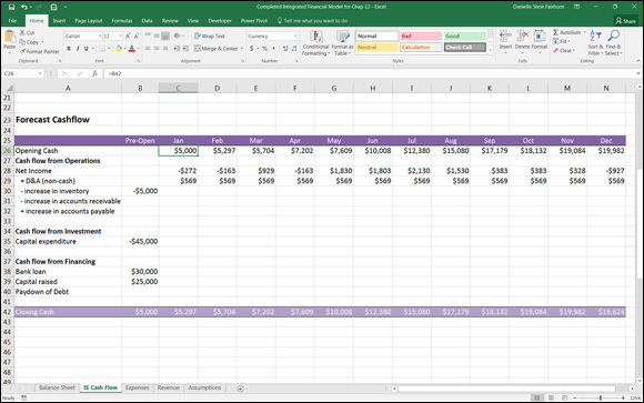
FIGURE 10-10: The completed cash flow statement.
Building the Balance Sheet
The accounting equation as shown on the balance sheet is perhaps the single most important concept to understand in terms of financial statements modeling:
Assets = Liabilities + Shareholders’ Equity
Let’s take a look at each of these components:
-
Assets: All property owned by the company. This includes cash in the bank, factories, materials, and even money you’re owed. You can think of assets as the resources that are used to generate revenue.
Assets are split into two categories:
- Current assets: Current assets can be easily converted into liquid assets or cash. This includes assets such as stocks and shares, account receivables (money that is owed to the company), and stock that will sell soon for cash.
- Fixed assets: Fixed assets are still property owned by the company, but they may take longer to convert into liquid assets. This includes large capital items such as factories or equipment, as well as nonphysical assets such as intellectual property or goodwill.
- Liabilities: All debts owed. Similarly, current liabilities are short-term debt that needs to be paid back within a year, such as accounts payable (money you owe to suppliers), credit card debt, or overdrafts. Long-term liabilities are more formal borrowings such as bank loans.
- Shareholders’ equity: What the owner has after all the debt has been repaid. If the company were sold, theoretically, this is what the shareholders would have.
The balance sheet shows the financial position of a company at any given moment. Just as with the income statement, the elements of a balance sheet need to be arranged in a specific order:
- ASSETS
- Current Assets
- Fixed Assets
- LIABILITIES
- Current Liabilities
- Long-Term Liabilities
- EQUITY
- Common Stock
- Additional Paid in Capital
- Retained Earnings
- TOTAL EQUITY
- TOTAL LIABILITIES AND EQUITY
Now that you’ve projected your income and cash flow, you need to complete your balance sheet and connect all three financial statements.
Your cafe’s beginning balance sheet at Year 0 will be tied to your sources and uses of funds. Your uses of funds will be your starting assets, and your sources of funds will represent your liabilities and equity. Breaking down the concepts, your uses of funds are assets that you’re purchasing in order to operate the business. Your sources of funds are how you fund the purchases of said assets — money can be raised through liabilities that you owe, such as a bank loan, or it can be equity invested by an owner (in this case, you!).
Start with the current assets (which for your business consists of your cash) and inventory. Follow these steps:
-
On the Balance Sheet worksheet, select cell B5 and enter the formula =‘IS Cash Flow’!B42.
This formula links cell B5 to the closing cash amount you calculated in the last section on the cash flow statement. This represents the starting cash of $5,000 your business has on hand.
-
Select cell B6 and enter the formula =K10.
This formula links cell B6 to the working inventory on the uses of funds you entered earlier on the same worksheet. This represents your starting inventory amount of $5,000.
- Leave accounts receivable in cell B7 blank, and sum the current assets in cell B8 with the formula =SUM(B5:B7); copy the formula across to the second year.
-
Select cell B11 and add cells K11 and K12 on the same worksheet with the formula =K11+K12.
The calculated value is $45,000. This represents your starting PP&E.
- Leave depreciation in cell B12 blank for now and sum the fixed assets net of depreciation with the formula =SUM(B11:B12); copy it across to the second year.
-
Sum the current and fixed assets in cell B15 with the formula =B13+B8; copy it across to the second year.
This gives you the calculated total asset value of $55,000.
- Leave row 20 blank because you don’t have any current liabilities at this point.
-
Select cell B23 and enter =K3.
This formula links cell B23 to the bank loan amount of $30,000 you entered earlier into the sources of funds section on the same worksheet. This represents the amount you have borrowed from, and owe to, the bank.
-
Sum total long-term liabilities in cell B24 with the formula =SUM(B23) and copy it across to the second year.
It may seem strange to only sum one number, but it’s important to do so for consistency. If at a later date you add other rows for long-term liabilities, they’ll also be included in this total.
-
Select cell B27 and enter the formula =K4.
This formula links cell B27 to the $25,000 equity amount raised that you entered earlier in the sources of funds section on the same worksheet. This represents the amount you’ve invested and your equity in the business.
-
Row 28 relates to retained earnings, which will come from the profit shown on the income statement.
This is not relevant for Year 0 because you haven’t yet begun operations.
-
Sum total the liabilities and equity in cell B31 with the formula =B29+B24, and copy it across to the second year.
You know that total assets must be equal to liabilities and equity in order for the balance sheet to balance, so this is a perfect opportunity to include an error check.
-
Add an error check in cell B32 with the formula =B31-B15 and copy it across to the second year.
Now that you’ve completed the balance sheet for the pre-open year, you need to link your balance sheet to the income and cash flow statements to determine what the balance sheet will look like after the first year of operations.
The cafe’s cash at bank will change by the amount of cash flow from your cash flow statement. You’ve already calculated this on a monthly basis, and you have a closing cash figure at the end of December of Year 1.
- Go back to the top of your balance sheet, select cell C5, and link it to the closing cash balance of $19,624 on the IS Cash Flow worksheet with the formula =‘IS Cash Flow’!N42.
-
In cell C11, enter the formula =-SUM(‘IS Cash Flow’!C35:N35).
This formula calculates the total amount of fixed assets on the books at the end of the second year. If you’ve purchased additional assets during the year, it will show on the cash flow statement, so you need to link that through with the formula. Note that any CapEx purchases on the cash flow statement are shown as negative values so you need to add a minus sign to the beginning of the sum to show it as a positive value. The total will be zero at this point, but that may change in future iterations of these financial statements.
You also need to add the existing fixed asset amount of $45,000 carried over from the previous year.
-
Add this amount to the beginning of the formula you already have in C11 so that it looks like this: =B11-SUM(‘IS Cash Flow’!C35:N35).
Note that fixed assets need to be shown at their original cost (regardless of whether they’ve increased or decreased in value since purchase) and then the accumulated depreciation is shown on a separate line to give us the total written-down value of the asset at that point in time. A long-term asset like the ones shown here will be depreciated until it’s worth nothing on the balance sheet at the end of its useful life.Because the fixed assets’ value is depreciated, you need to pick up the D&A amount already calculated on the income statement.
-
Select cell C12 and enter the formula =-’IS Cash Flow’!O13.
You need to enter the minus sign because D&A subtracts from gross PP&E.
-
Check your totals.
The total amount of D&A expensed throughout Year 1 is $6,833, total fixed assets is $38,167, and total assets is $62,791.
Moving on to liabilities, in cell C23 you need to take into consideration any paying down of debt that may have occurred during the year. If there is any, it would show up in the cash flow on row 40.
-
Although there isn’t any at the moment, you should still link this row through to the balance sheet with the formula =SUM(‘IS Cash Flow’!C40:N40).
The calculated value is zero.
-
You then need to add the bank loan carried over from the previous year, so adjust the formula in cell C23 to =B23+SUM(‘IS Cash Flow’!C40:N40).
The calculated value is $30,000.
-
For owners’ funds in cell C27, simply carry this over to the next year with the formula =B27.
Finally, your retained earnings represent the amount of economic profit, or net income, your business has earned that has been retained in the company. This can be kept in the company to reinvest in the business or pay down debt, or it can be paid out as dividends to shareholders.
-
Select cell C28 and link it to cell O20 on the IS Cash Flow worksheet with the formula =‘IS Cash Flow’!O20.
The calculated value is $7,791 and represents the total net income earned throughout the year.
Congratulations! You’ve linked all three financial statements. Check your totals against Figure 10-11 and make sure that you perform a balance sheet error check to see if your total assets equal your total liabilities and equity, and thus balances.

FIGURE 10-11: The completed balance sheet.
The balance sheet check is the most important one because it’s the most common place where an error will surface due to the many moving pieces that all need to be correct in order for both sides of the balance sheet to balance. Many times, the error will be between the balance sheet and cash flow statement and may be because of an incorrect minus or positive value. When trying to reconcile a balance sheet that does not balance, I find it helpful to remember that the total assets must be equal to the total liabilities and equity, so if I add an item to the assets side of the equation, I need to add an amount of the same value to the other side of the equation.
Building Scenarios
Now that you’ve determined your base case assumptions that reflect how you believe the business will perform, you also want to run worst-case and best-case scenarios. Not only do you want to see how you believe the business will do, but you also want to see how the business will perform if it does worse than expectations or better than expectations.
Running multiple scenarios is a very important part of financial modeling — some would say it’s the whole point of financial modeling — because it allows the user to gauge the different outcomes if certain assumptions end up being different. Because no one can see into the future and assumptions invariably end up being wrong, being able to see what happens to the outputs when the main assumption drivers are changed is important.
Because you’ve built this integrated financial model such that all the calculations are linked either to input assumption cells, or to other parts of the financial statements, any changes in assumptions should flow nicely throughout the model. The proof is in the pudding, however. In this section, you see what happens when you make major changes to this model with scenario analysis!
Entering your scenario assumptions
Going back now to the Assumptions worksheet, you believe that the main drivers of profitability for your cafe will be the average number of cups you sell per day and the rent you’ll pay. You believe that reducing cups sold per day by 20 cups and increasing rent by 10 percent is a reasonable worst-case scenario, and increasing cups sold per day by 20 cups and reducing rent by 10 percent is a reasonable best-case scenario.
At the very top of the Assumptions worksheet, enter the scenario input assumptions as shown in Figure 10-12.

FIGURE 10-12: Scenario input assumptions.
Building a drop-down box
You’ve decided on your scenario assumptions, so now you need to build a drop-down box, which is going to drive your scenario analysis. You have a full, working financial model, so you want the ability to easily switch between your scenarios to see how the outputs change in real time. You can put the scenario drop-down box on either of the financial statements, but for this example you’ll put it at the top of the income statement.
Follow these steps:
- Go to the IS Cash Flow worksheet and select cell B1.
-
Select Data Validation in the Data Tools section of the Data Ribbon.
The Data Validation dialog box appears.
-
From the Allow drop-down list, select List.
You could type the words Best, Base, and Worst directly into the field, but it’s best to link it to the source in case you misspell a value. To review how to use a data validation drop-down box, turn to Chapter 6.
-
In the Source field, type = and then click the Assumptions worksheet, and highlight the scenario names Worst, Base, Best.
Your formula in the Source field should now be =Assumptions!$B$2:$D$2, as shown in Figure 10-13.
- Click OK.
- Go back to cell B1 on the IS Cash Flow worksheet, and test that the drop-down box is working as expected and gives the options Best, Base, and Worst.
- Set the drop-down box to Base for now.

FIGURE 10-13: Building the scenario drop-down box.
Building the scenario functionality
You need to edit your input assumptions for number of cups sold per day and monthly rent so that as the drop-down box on the IS Cash Flow worksheet changes, the input assumptions change to the corresponding scenario. For example, when Best has been selected on the IS Cash Flow worksheet, the value in cell B9 on the Assumptions worksheet should be 140, and the value in cell B23 should be $1,080. This should be done using a formula.
Often, many different functions will achieve the same or similar results. Which function you use is up to you as the financial modeler, but the best solution will be the one that performs the required functionality in the cleanest and simplest way, so that others can understand what you’ve done and why.
In this case, there are several options you could use: a HLOOKUP, a SUMIF, or an IF statement. In my opinion, the IF statement, being a nested function, is the most difficult to build and is less scalable. If the number of scenario options increase, the IF statement option is more difficult to expand. In this instance, I have chosen to use the HLOOKUP with these steps.
Follow these steps (and see Chapter 7 for more information on HLOOKUP):
- Select cell B9 and press the Insert Function button on the Formulas tab or next to the formula bar.
-
Search for HLOOKUP, press Go, and click OK.
The HLOOKUP dialog box appears.
-
Click the Lookup_value field, and select the drop-down box on the IS Cash Flow worksheet.
This is the criteria that drives the HLOOKUP.
-
Press F4 to lock the cell reference.
In the Table_array field, you need to enter the array you’re using for the HLOOKUP. Note that your criteria must appear at the top of the range.
-
Select the range that is the scenario table at the top — in other words, B2:D4 — and the press F4 to lock the cell references.
The cell references will change to $B$2:$D$4.
- In the Row_index_num field, enter the row number, 2.
- In the Range_lookup field, enter a zero or false, because you’re looking for an exact match.
- Check that your dialog box looks the same as Figure 10-14.
-
Click OK.
The formula in cell B9 is =HLOOKUP(‘IS Cash Flow’!B1,$B$2:$D$4,2,0) with the calculated result of 120.
-
Perform the same action in cell B23 with the formula =HLOOKUP(‘IS Cash Flow’!$B$1,$B$2:$D$4,3,0).
Instead of re-creating the entire formula again, simply copy the formula from cell B9 to cell B23 and change the row reference from 2 to 3. Copying the cell will change the formatting of the number, so you’ll need to change the currency symbol back to $ again. -
Go back to the IS Cash Flow worksheet and change the drop-down to Best.
Check that your assumptions for average number of cups sold per day and monthly rent on the Assumptions worksheet have changed accordingly. Cups will have changed to 140 and rent to $1,080.
Now, the important test is to see if the balance sheet still balances!
- Go back to the Balance Sheet worksheet and make sure that your error check is still zero.
-
Test the drop-down again by changing it to Worst.
Cups will have changed to 100 and rent will be $1,320. Check the error check on the Balance Sheet worksheet again.

FIGURE 10-14: Building a scenario with HLOOKUP.
Congratulations! Your entirely integrated financial model, together with scenario analysis, is now complete! You can download a copy of the completed model in File 1002.xlsx at www.dummies.com/go/financialmodelinginexcelfd.