
1
Signal Generation in Radiation Detectors
Understanding pulse formation mechanisms in radiation detectors is necessary for the design and optimization of pulse processing systems that aim to extract different information such as energy, timing, position, or the type of incident particles from detector pulses. In this chapter, after a brief introduction on the different types of radiation detectors, the pulse formation mechanisms in the most common types of radiation detectors are reviewed, and the characteristics of detectors’ pulses are discussed.
1.1 Detector Types
A radiation detector is a device used to detect radiation such as those produced by nuclear decay, cosmic radiation, or reactions in a particle accelerator. In addition to detecting the presence of radiation, modern detectors are also used to measure other attributes such as the energy spectrum, the relative timing between events, and the position of radiation interaction with the detector. In general, there are two types of radiation detectors: passive and active detectors. Passive detectors do not require an external source of energy and accumulate information on incident particles over the entire course of their exposure. Examples of passive radiation detectors are thermoluminescent and nuclear track detectors. Active detectors require an external energy source and produce output signals that can be used to extract information about radiation in real time. Among active detectors, gaseous, semiconductor, and scintillation detectors are the most widely used detectors in applications ranging from industrial and medical imaging to nuclear physics research. These detectors deliver at their output an electric signal as a short current pulse whenever ionizing radiation interacts with their sensitive region. There are generally two different modes of measuring the output signals of active detectors: current mode and pulse mode. In the current mode operation, one only simply measures the total output electrical current from the detector and ignores the pulse nature of the signal. This is simple but does not allow advantage to be taken of the timing and amplitude information that is present in the signal. In the pulse mode operation, one observes and counts the individual pulses generated by the particles. The pulse mode operation always gives superior performance in terms of the amount of information that can be extracted from the pulses but cannot be used if the rate of events is too large. Most of this book deals with the operation of detectors in pulse mode though the operation of detectors in current mode is also discussed in Chapter 5. The principle of pulse generation in gaseous and semiconductor detectors, sometimes known as ionization detectors, is quite similar and is based on the induction of electric current pulses on the detectors’ electrodes. The pulse formation mechanism in scintillation detectors involves the entirely different physical process of producing light in the detector. The light is then converted to an electric current pulse by using a photodetector. In the next sections, we discuss the operation of ionization detectors followed by a review of pulse generation in scintillation detectors and different types of photodetectors.
1.2 Signal Induction Mechanism
1.2.1 Principles
In gaseous and semiconductor detectors, an interaction of radiation with the detector’s sensitive volume produces free charge carriers. In a gaseous detector, the charge carriers are electrons and positive ions, while in the semiconductor detectors electrons and holes are produced as result of radiation interaction with the detection medium. In such detectors, an electric field is maintained in the detection medium by means of an external power supply. Under the influence of the external electric field, the charge carriers move toward the electrodes, electrons toward the anode(s), and holes or positive ions toward the cathode(s). The drift of charge carriers leads to the induction of an electric pulse on the electrodes, which can be then read out by a proper electronics system for further processing. To understand the physics of pulse induction, first consider a charge q near a single conductor as shown in Figure 1.1. The electric force of the charge causes a separation of the free internal charges in the conductor, which results in a charge distribution of opposite sign on the surface of the conductor. The geometrical distribution of the induced surface charge depends on the position of the external charge q with respect to the conductor. When the charge moves, the geometry of charge conductor changes, and therefore, the distribution of the induced charge varies, but the total induced charge remains equal to the external charge q. We now consider a gaseous or semiconductor detector with a simple electrode geometry including two conductors as shown in Figure 1.2. If an external charge q is placed at distance x∘ from one electrode, charges of opposite sign with the external charge are induced on each electrode whose amount and distribution depends on the distance of the external charge from the electrode [1]:
and
where d is the distance between the two electrodes. When the external charge moves between the electrodes, the induced charge on each electrode varies, but the sum of induced charges remains always equal to the external charge q = q1 + q2. If two electrodes are connected to form a closed circuit, the changes in the amount of induced charges on the electrodes lead to a measurable current between the electrodes. As it is illustrated in Figure 1.2, when the external charge is initially close to the upper electrode, most of the field strength will terminate there and the induced charge will be correspondingly higher, but as the charge moves toward the lower electrode, the charge induced on the lower electrode increases. This means that the polarity of outgoing charges from electrodes or the observed pulses are opposite. In general, the polarity of the induced current depends on the polarity of the moving charge and also the direction of its movement in respect to the electrode. As a rule, one can remember that a positive charge moving toward an electrode generates an induced positive signal; if it moves away, the signal is negative and similarly for negative charge with opposite signs. In a radiation detector, a radiation interaction produces free charge carriers of both negative and positive signs. The motion of positive and negative charge carriers toward their respective electrodes increases their surface charges, the cathode toward more negative and the anode toward more positive, but by moving the charge away from the other electrode, the charge of opposite polarity is induced on that electrode. The total induced charge on each electrode is due to the contributions from both types of charge carriers, which are added together due to the opposite direction and opposite sign of the charges.

Figure 1.1 The induction of charge on a conductor by an external positive charge q (top) and the density of the induced surface charge on the conductor (bottom).

Figure 1.2 The induction of current by a moving charge between two electrodes. When charge q is close to the upper electrode, the electrode receives larger induced charge, but as the charge moves toward to the bottom electrode, more charge is induced on that electrode. If the two electrodes are connected to form a closed circuit, the variations in the induced charges can be measured as a current.
The start of a detector output pulse, in most of the situations, is the moment that radiation interacts with the detector because the charge carriers immediately start moving due to the presence of an external electric field. The pulse induction continues until all the charges reach the electrodes and get neutralized. Therefore, the duration of the current pulse is given by the time required for all the charge carriers to reach the electrodes. This time is called the charge collection time and is a function of charge carriers’ drift velocity, the initial location of charge carriers, and also the detector’s size. The charge collection time can vary from a few nanoseconds to some tens of microseconds depending on the type of the detector. By integrating the current pulse generated in the detector, a net amount of charge is produced, which would be equal to the total released charge inside the detector if all the charge carriers are collected by the electrodes. In most of the detectors, there is a unique relationship between the energy deposited by the radiation and the amount of charge released in the detector, and therefore, the deposited energy can be obtained from the integration of the output current pulse. Figure 1.3 shows the induced pulses when a detector’s electrode is segmented. The amplitude of the pulse induced on each segment will depend upon the position of the charge with respect to the segment. As the charge gets closer to the electrode, the charge distribution becomes more peaked, concentrating on fewer segments. Therefore, with a proper segmentation of the electrode, one can obtain information on the location of radiation interaction in the detector by analyzing the induced signals on the electrode’s segments. This is called position sensing and such detectors are called position sensitive. Detectors with electrodes divided to pixels or strips are the most common types of designs for position sensing in radiation imaging applications. It should be also mentioned that the induction of signal on a conductor is not limited to the electrodes that maintain the electric field in the detector. In fact, any conductor, even without connection to the power supply, can receive an induced signal. This property is sometimes used to acquire extra information on the position of incident particles on the detectors.

Figure 1.3 The induction of pulses on the segments of an electrode. In a segmented electrode, charge is initially induced on many segments, but as the charge approaches the electrode, the largest signal is received by the segment, which has the minimum distance with the charge.
The induced charge on an electrode by a moving charge q can be computed by using the electrostatic laws. This approach is illustrated in Figure 1.4 where the charge q is shown in front of an electrode. The induced charge Q on the electrode can be calculated by using Gauss’s law. Gauss’s law says that the induced charge on an electrode is given by integrating the normal component of the electric field E over the Gaussian surface S that surrounds the surface of the electrode:
where ε is the dielectric constant of the medium. The time‐dependent output signal of the detector can be obtained by calculating the induced charge Q on the electrode as a function of the instantaneous position of the moving charges between the electrodes of the detector. However, this calculation process is very tedious because one needs to calculate a large number of electric fields corresponding to different locations of charges along their trajectory to obtain good precision. A more convenient method for the calculation and description of the induced pulses is to use the Shockley–Ramo theorem. The method is described in the next section, and its application to some of the common types of gaseous and semiconductor detectors are shown in Sections 1.3.1 and 1.3.2.

Figure 1.4 The calculation of induced charge on an electrode by using Gauss’s law.
1.2.2 The Shockley–Ramo Theorem
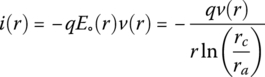
Shockley and Ramo separately developed a method for calculating the charge induced on an electrode in vacuum tubes [2, 3], which was then used for the explanation of pulse formation in radiation detectors. Since then, several extensions of the theorem have been also developed, and it was proved that the theorem is valid under the presence of space charge in detectors. The proof and some recent reviews of the Shockley–Ramo theorem can be found in Refs. [4–6]. In brief, the Shockley–Ramo theorem states that the instantaneous current induced on a given electrode by a moving charge q is given by
and the total charge induced on the electrode when the charge q drifts from location xi to location xf is given by
In the previous relations, v is the instantaneous velocity of charge q and φ∘ and E∘ are, respectively, called the weighting potential and the weighting field. The weighting field and the weighting potential are a measure of electrostatic coupling between the moving charge and the sensing electrode and are the electric field and potential that would exist at q’s instantaneous position x under the following circumstances: the selected electrode is set at unit potential, all other electrodes are at zero potential, and all external charges are removed. One should note that the actual electric field in the detector is not directly present in Eq. 1.4, but it is indirectly present because the charge drift velocity is normally a function of the actual electric field inside the detector. In the application of the Shockley–Ramo theorem to radiation detectors, the magnetic field effects of the moving charge carriers are neglected because the drift velocity of the moving charge carriers is low compared with the velocity of light. For example, in germanium the speed of light is 750 × 107 cm/s, while the drift velocity of electrons and holes is less or comparable with 107 cm/s. The calculation of weighting fields and potentials in simple geometries such as planar and cylindrical electrodes can be analytically done, which enables one to conveniently compute the time‐dependent induced pulses. In the case of more complex geometries such as segmented electrodes with strips or pixel structure, one can use electrostatic field calculation methods that are now available as software packages. In the following sections, we will use the concept of weighting fields and potentials for calculating the output pulses for some of the common types of gaseous and semiconductor detectors, but before that we describe how a detector appears as source of signal in a detector circuit.
1.2.3 Detector as a Signal Generator
We have so far discussed that ionization detectors produce a current pulse in response to an interaction with the detector. Therefore, detectors can be considered as a current source in the circuit. Figure 1.5 shows the basic elements of a detector circuit together with its equivalent circuit. The detector exhibits a capacitance (Cd) in the circuit to which one can add the sum of other capacitances in the circuit including the capacitance of the connection between the detector and measuring circuit and stray capacitances present in the circuit. The detector also has a resistance shown by Rd. The bias voltage is normally applied through a load resistor (RL), which in the equivalent circuit lies in parallel with the resistor of the detector. In a similar way, the measuring circuit, which is normally a preamplifier, has an effective input resistance, Ra, and capacitance, Ca. When the detector is connected to the measuring circuit, the equivalent input resistance, R, and capacitance, C, are obtained by combining all the resistors and capacitances at the input of the measuring circuit. In the equivalent circuit it is shown that the total resistance (R) and capacitance (C) form an RC circuit with a time constant τ = RC. The current pulse induced by the moving charge carriers on the detector’s electrodes appears as a voltage pulse at the input of the readout electronics. The shape of this voltage pulse is a function of the time constant of the detector circuits. If the time constant is small compared with the duration of charge collection time in the detector, then the current flowing to the resistor is essentially equal to the instantaneous value of the current flowing in the detector, and thus the measured voltage pulse has a shape nearly identical to the time dependence of the current produced within the detector. This pulse is called current pulse. If the time constant is larger than the charge collection time, which is a more general case, then the current is integrated on the total capacitor, and therefore it represents the charge induced on the electrode. This pulse is called charge pulse. The integrated charge will finally discharge on the resistor, leading to a voltage that can be described as
where Q∘ is the total charge produced in the detector. Because the capacitance C is normally fixed, the amplitude of the signal pulse is directly proportional to the total charge generated in the detector:

Figure 1.5 The arrangement of a detector–preamplifier and its equivalent circuit.
Bearing in mind that the total charge produced in the detector is proportional to the energy deposited in the detector, Eq. 1.7 means that the amplitude of the charge pulse is proportional to the energy deposited in the detector.
1.3 Pulses from Ionization Detectors
1.3.1 Gaseous Detectors
The physics of gaseous detectors have been described in various excellent books and reviews (see, e.g., Refs. [7, 8]). Here only a quick overview of the principles is given and more detailed information can be found in the references. The operation of a gaseous detector is based on the ionization of gas molecules by radiation, producing free electrons and positive ions in the gas, commonly known as ion pairs. The average number of ion pairs due to a radiation energy deposition equal to ΔE in the detector is given by
where w is the average energy required to generate an ion pair. The w‐value is, in principle, a function of the species of gas involved, the type of radiation, and its energy. The typical value of w is in the range of 23–40 eV per ion pair. The production of ion pairs is subject to statistical variations, which are quantified by the Fano factor. The variance of the fluctuations in the number of ion pairs is expressed in terms of the Fano factor F as
The Fano factor ranges from 0.05 to 0.2 in the common gases used in gaseous detectors. Under the influence of an external electric field, the electrons and positive ions move toward the electrodes, inducing a current on the electrodes. If the external electric field is strong enough, the drifting electrons may produce extra ionization in the detector, thereby increasing the amount of induced signal. Depending on the relation between the amount of initial charge released in the detector and total charge generated in the detector, the operation of gaseous detectors can be classified into three main regions including ionization chamber region, proportional region, and Geiger–Müller (GM) region. This classification is illustratively shown in Figure 1.6. At very low voltages, the ion pairs do not receive enough electrostatic acceleration to reach the electrodes and therefore may combine together to form the original molecule, instead of being collected by the electrodes. Therefore, the total collected charge on the electrodes is less than the initial ionization. This region is called region of recombination, and no detector is practically employed in this region. In the second region, the electric field intensity is only strong enough to collect all the primary ion pairs by minimizing the recombination of electron ion pairs. The detectors operating in this region are called ionization chambers. When the electric field is further increased, the electrons gain enough energy to cause secondary ionization. This process is called gas amplification or charge multiplication process. As a result of this process, the collected charge will be larger than the amount of initial ionization, but it is linearly proportional to it. The detectors operating in this region are called proportional counters. The operation of a detector in the proportional region is characterized by a quantity called first Townsend coefficient (α), which denotes the mean number of ion pairs formed by an electron per unit of its path length. The first Townsend coefficient is a function of gas pressure and electric field intensity, and therefore, the operation of a proportional counter is governed by the gas pressure and the applied voltage. By having the first Townsend coefficient, the increase in the number of electrons drifting from location x1 to location x2 is characterized with a charge multiplication factor A given by

and the total amount of charge Q generated by n∘ original ion pairs is obtained as

Figure 1.6 The classification of gaseous detectors based on the amount of charge generated in the detector for a given amount of ionization.
From this relation, it follows that the amount of charge generated in the detector can be controlled by the gas amplification factor, but one should know that the maximum gas amplification is practically limited by the maximum amount of charge that can be generated in a gaseous detector before the electrical breakdown happens. This is called the Raether limit and happens when the amount of total charge reaches to ~108 electrons [9]. Even before reaching to the Raether limit, the increase in the applied voltage leads to nonlinear effects, and a region called limited proportionality starts. The nonlinear region stems from the fact that opposite to the free electrons, which are quickly collected due to their high drift velocity, the positive ions are slowly moving and their accumulation inside the detector during the charge multiplication process distorts the external electric field and consequently the gas amplification process. When the multiplication of single electrons is further increased (106–108), the detector may enter to the GM region. In this regime, the gas amplification is so high that the photons whose wavelength may be in visible or ultraviolet region are produced. By means of photoionization, the photons may produce new electrons that initiate new avalanches. Consequently, avalanches extend in the detector volume and very large pulses are produced. This process is called a Geiger discharge. Eventually, the avalanche formation stops because the space‐charge electric field of the large amount of positive ions left behind reduces the external electric field, preventing more avalanche formation. As a result, a detector operating in the Geiger region gives a pulse whose size does not depend on the amount of primary ionization. The shape of a pulse for a gaseous detector depends not only on its operating region but also on its electrode geometry. In the following sections, we will review the pulse‐shape characteristics of gaseous detectors of common geometries, operating in different regions.
1.3.1.1 Parallel‐Plate Ionization Chamber
Ionization chambers are among the oldest and most widely used types of radiation detectors. Ionization chambers offer several attractive features that include variety in the mode of signal readout (pulse and current mode) and extremely low level of performance degradation due to the radiation damage, and also these detectors can be simply constructed in different shapes and sizes suitable for the application. Here, we discuss the pulse formation in an ionization chamber with parallel‐plate geometry, and description of pulses from other geometries such as cylindrical can be found in Ref. [10].
As it is shown in Figure 1.7, the detector consists of two parallel electrodes, separated by some distance d. The space between the electrodes is filled with a suitable gas. We will assume that d is small compared with both the length and width of the electrodes so that the electric field inside the detector is uniform and normal to the electrodes, with magnitude
where V is the applied voltage between the electrodes. For the purpose of pulse calculation, we initially assume that all ion pairs are formed at an equal distance x∘ from the anode. In this way, an ionization electron will travel a distance x∘ to the anode, and a positive ion travels a distance d – x∘ to the cathode. The drift time Te for an electron to travel to the anode depends linearly on x∘ as
where ve is the electron’s drift velocity. The ions reach the cathode in a time Tion:
where vion is the drift velocity of positive ions. The current induced on the electrodes of an ionization chamber is due to the drift of both electrons and positive ions. To calculate the current ie induced on the anode electrode due to n∘ drifting electrons by the Shockley–Ramo theorem, one needs to determine the anode’s weighting field. The weighting field E∘ is obtained by holding the anode electrode at unit potential and the cathode electrode is grounded. By setting V = 1 in Eq. 1.12, E∘ is simply given as

Figure 1.7 The cross section of a parallel‐electrode ionization chamber used in deriving the shape of pulses induced by ion pairs released at the distance x∘ from the anode of the detector.
Since the directions of the electrons’ drift velocity and the external electric field are opposite, Eq. 1.4 gives the current induced by the electrons on the anode as
The negative sign of n∘e is due to the negative charge of electrons. Once an electron reaches the anode, it no longer induces a current on the anode and therefore ie = 0 for t > te. Equation 1.16 indicates that the polarity of the pulse induced on the anode is negative, which is in accordance with the rule that we mentioned in Section 1.2.1. If we calculate the current induced on the cathode by electrons, the drift velocity of electrons and the weighting field are in the same direction, and thus, the polarity of induced charge will be positive. The induced current by positive ions on the anode can be similarly calculated as
The total induced current on the anode is a sum of contributions from electrons and positive ions, given by
The top panel of Figure 1.8 shows an example of induced currents on the anode of an ionization chamber. The figure shows a hypothetical case in which the drift velocity of electrons is only five times larger than that of positive ions. In practice, the drift velocity of electrons is much larger than positive ions (~1000 times), and thus the induced current by positive ions has much smaller amplitude and much longer duration. The calculated induced currents have constant amplitude because of the constant drift velocity of charge carriers and have zero risetimes though this cannot be practically observed due to the finite bandwidth of the detector circuit. The charge pulse induced on the electrodes as a function of time can be obtained by using the Shockley–Ramo theorem (Eq. 1.5) or alternatively by a simple integration of the calculated induced currents. The integral of ie(t) over time, which we denote it as Qe(t), represents the induced charge on the anode due to the n∘ drifting electrons as


Figure 1.8 (Top) Time development of an induced current pulse on the anode of a planar ionization chamber by the motion of electrons and positive ions. The figure is drawn as if the electron drift velocity is only five times faster than the ion drift velocity. (Bottom) The induced charge on the anode.
The polarity of this pulse is opposite to the polarity of induced charge, which is obtained from Eq. 1.5. This is due to the fact that the Shockley–Ramo theorem gives the total induced charge on the electrode, while the integration of current pulse represents the outgoing charge from the electrode or the observed pulse. The induced charge increases linearly with time until electrons reach the anode after which the charge induced by electrons remains constant. Similarly, the induced charge Qion(t) by the drift of positive ions is given by

The positive ion pulse also linearly increases with time, but with a smaller slope due to the smaller drift velocity of positive ions. The total induced charge on the anode, during the drift of electrons and positive ions, is obtained as
After the electrons’ collection time, Te, the electrons have contributed to the maximum possible value, and the electron contribution becomes constant. But if the positive ions are still drifting, Eq. 1.21 takes the form
When both the electrons and ions reached their corresponding electrodes, Eq. 1.22 is written as
The bottom panel of Figure 1.8 shows the time development of the charge pulse on the anode electrode. The final amount of charge is equal to the total charge generated in the detector. As it was discussed before, in practice, one measures a voltage at the output of the detector circuit (charge pulse) whose amplitude is proportional to the initial ionization if the time constant of the circuit is sufficiently long. The effect of the time constant is shown in Figure 1.9. If the time constant is very large (RC ≫ Tion), the amplitude of the pulse is proportional to the initial amount of ionization (Vmax = n∘e/C). In the case that the time constant of the detector bias circuit is comparable with or smaller than the charge collection time (RC ≤ Tion), the voltage pulse will decay without reaching to its maximum value, and therefore, the proportionality of pulse amplitude with the energy deposition in the detector is lost. This is particularly a serious problem in ionization chambers because the very small drift velocity of positive ions necessitates the use of a very long time constants, in the range of milliseconds, but a very long time constant sets a serious limit for the operation of ionization chambers at a decent count rate.

Figure 1.9 The output voltage pulse of an ionization chamber for different circuit time constants.
The shape of pulses calculated so far represents simple cases in which ionization is produced at the same distance from the electrodes or at a single point in the detector. However, ionization chambers are widely used for charged particle detection for which the initial ionization can have a considerable distribution between the electrodes. Therefore, the shapes of pulses would be slightly different from the calculated pulses. However, the expressions for a point‐like ionization permit to compute the induced charge and currents for extended ionization tracks as those produced by charged particles. The computation is based on the division of the particle track to point‐like ionizations and taking the superposition of currents (or charges) induced by point‐like ionizations. In this way, the electron component of induced current for particle track can be described by the following integral:

where ρ(x) denotes the geometrical distribution of ionization extended from location x1 to location x2 from the anode. A similar approach can be used to compute the induced current by positive ions.
1.3.1.2 Gridded Ionization Chamber
The problem of long collection time of positive ions in ionization chambers can be alleviated by placing a wire (Frisch) grid very close to the anode of the chamber. Such detector structure is called gridded ionization chamber and is schematically shown in Figure 1.10. Radiation interaction with the detector takes place in the space between the grid and cathode, and by applying proper bias voltages between the electrodes, the released electrons pass through the openings of the Frisch grid to be finally collected by the anode. The shape of the charge pulses induced on the anode of a gridded ionization chamber can be easily calculated by using Eq. 1.5. The weighting potential of the anode is obtained by applying a unit potential on the anode and zero potential on both the grid and the cathode. The weighting potential is zero between the cathode and the grid and rises linearly to unity from the grid to the anode as shown in the bottom of Figure 1.10. This configuration of weighting potential means that a charge moving between the cathode and the grid causes no induced charge on the anode and only those electrons passed through the grid contribute to the anode signal. Therefore, the dependence of the output pulse to slow drifting positive ions is completely removed. The time‐dependent induced charge on the anode is given by
where d is the grid–anode spacing. One should note that polarity of the induced charge on the conductor is opposite to the polarity of the observed pulse. The slope of the pulse does not change and the linear rise of the pulse continues until electrons are collected on the anode, which can take quite a short time, about 1 µs. The total induced charge when the electrons reach the anode is n∘e, indicating that the proportionality between the amount of primary ionization and the pulse amplitude is maintained though the pulse is merely induced by electrons.

Figure 1.10 The structure of gridded ionization chamber and the weighting potential of the anode.
A gridded ionization chamber is an example detector in which the moment of the appearance of the pulse is different from the moment of radiation interaction with the detector. This difference is because the pulse on the anode only appears when electrons pass through the wire grid while electrons released by radiation interaction need some time to reach the grid. This mechanism of pulse formation produces a useful property in the applications involving charged particles. Figure 1.11 shows the shape of a current pulse from a charged particle in such detector. The ionization produced by charged particles has a sizable distribution according to the particles’ Bragg peak shape, and the output pulse is determined by the superposition of point‐like ionizations that form the Bragg curve. Since the drift time of electrons to the wire grid depends on the shape of the Bragg curve, the superposition of the currents due to point‐like ionizations will also represent the Bragg curve of the particle, which can be then used to identify the charged particle. Due to this property, gridded ionization chambers are sometime called Bragg curve spectrometer (BCC) and are widely used as a heavy ion detector in the field of nuclear physics [11].

Figure 1.11 Schematic drawing of the relationship between a particle’s Bragg peak and the shape of a current pulse from a BCS detector.
1.3.1.3 Parallel‐Plate Avalanche Counter
The multiplication of electrons in a gaseous detector operating in the proportional region can be performed in various electric field geometries. A parallel‐plate avalanche counter is a proportional counter in which the multiplication of electrons takes place in a uniform electric field. In X‐ray detection applications, the multiplication gap is coupled to a conversion region, in which ion pairs are created. The length of conversion region is chosen to achieve the required detection efficiency. The separation of the conversion and the multiplication gaps is made by using a wire mesh or a grid of thin wires. The structure of such detector and the electric field distribution are shown in Figure 1.12. When a proper uniform electric field toward the wire mesh is maintained in the conversion gap, the electrons produced in the conversion gap pass through the openings of the wire mesh and enter the multiplication gap where the electric field is strong enough for charge multiplication. The charge multiplication takes place according to Eq. 1.10 with a constant Townsend coefficient value because the electric field in the multiplication gap is constant. The multiplication factor is given by

where x is the distance traveled by electrons in the multiplication gap, ve is the drift velocity of electrons, and t is the time elapsed after the start of charge multiplication. Starting from n∘ primary electrons, the number of electrons as a function of time will be then given by

Figure 1.12 The structure and distribution of electric field in a parallel‐plate avalanche counter designed for X‐ray detection.
To calculate the current induced by electrons on the wire grid, we use the weighting field E∘ = 1/d where d is the thickness of the multiplication gap. By having the weighting field and the instantaneous number of electrons, the current induced by electrons on the wire grid is given by the Shockley–Ramo relation as
where Te is the electrons’ collection time given by d/ve. The contribution to the induced current by the positive ions can be also calculated by having the instantaneous number of positive ions. The instantaneous number of positive ions is calculated by taking into account the exponential growth in the number of positive ions during the charge multiplication process and the gradual collection of positive ions at the wire grid. The induced current pulse by positive ions is given by [9, 12]
with
where vion and Tion are, respectively, the drift velocity and collection time of positive ions. The top panel of Figure 1.13 shows the induced currents by electrons and positive ions computed for a hypothetical case in which the drift velocity of electrons is only five times larger than the drift velocity of positive ions. In practice, the drift velocity of electrons is significantly larger than that of positive ions, and therefore, the amplitude of the electrons’ current pulse is significantly larger than that for positive ions. One can see that due to the multiplication of electrons, the electron current pulse has a nonzero risetime, which is different from the current pulse from ionization chambers. The induced charge pulse can be obtained by the integration of the current pulses over the charge collection time as
and


Figure 1.13 (Top) The electron‐ and positive ion‐induced current pulses in a parallel‐plate avalanche counter. (Bottom) The time development of a charge pulse in a parallel‐plate avalanche counter.
The shape of the charge pulse is shown in the bottom panel of Figure 1.13. It is important to note that while the electron contribution is prominent in the current pulse, the charge pulse is mainly formed by the drift of positive ions. This is explained by the fact that due to the exponential growth in the number of electrons, the majority of electrons are produced very close to the anode, and thus they travel very short distance before they are collected by the anode. The small drift distance makes their charge induction very small as it is expected from Eq. 1.5.
Avalanche counters are also widely used for the detection of heavily ionizing charged particles. In charged particle detection applications, a conversion gap is not required as charged particles are directly ionizing particles that can produce enough number of ion pairs in a thin multiplication gap even at low gas pressures. Therefore, the detector structure is simplified to two parallel electrodes. Such detectors are normally used in transmission mode, which means that charged particles traverse the small gap of the detector as shown in the inset of Figure 1.14. By assuming that in a thin gap of a low‐pressure gas the ionization has a uniform distribution, the instantaneous number of electrons ne(t) is calculated as
where the first term describes the multiplication and the second term describes the collection of the electrons. By using the weighting field 1/d, the electron current pulse on the anode is calculated as

Figure 1.14 A transmission avalanche counter and the shape of current and charge pulses induced by a charged particle.
To calculate the instantaneous number of positive ions, one can assume that the electron multiplication and electron collection occur instantaneously at time zero in comparison with positive ions’ slow motion to the cathode. In this case, the current pulse induced by the motion of positive ions is calculated as [13]
The charge induced on the electrodes by electrons and positive ions are also calculated by integrating the current pulses as

The total charge pulse is the sum of Qe and Qion. The shape of induced current and charge pulses in a transmission parallel‐plate avalanche counter are shown in Figure 1.14. The pulse is very similar to that calculated for X‐ray detection with the difference that the maximum of electron current pulse happens before the electron collection time.
The extended surface of electrodes in proportional counters with parallel‐plate geometry increases the probability of destructive electric discharges that can happen between the electrodes. A variant of detectors with parallel‐plate geometry is resistive plate chamber (RPC) in which the electrodes are made of high resistivity materials such as Bakelite. In such detectors, when a discharge happens in the detector, due to the high resistivity of the electrodes, the electric field is suddenly dropped in a limited area around the point where the discharge occurred. Thus the discharge is prevented from propagating through the whole gas volume. The formation of pulses can be described by using the Shockley–Ramo theorem, but it requires the calculation of the instantaneous number of charge carriers, actual electric field, and other details in the operation of the detector, which have been implemented in some simulation studies [14].
1.3.1.4 Cylindrical Proportional Counter
Gaseous detectors with cylindrical geometry operating in the proportional region have been widely used for different radiation detection applications such as X‐ray and neutron detection. An illustration of a cylindrical proportional counter and its schematic cross section is shown in Figure 1.15. The detector consists of a cylindrical cathode with a central anode wire. The diameter of anode wire is typically 10–30 µm and the diameter of the cathode is typically a few centimeters. Anode is biased at a high voltage and the cathode is normally grounded. The electric field in such geometry is increasing toward the anode wire. Under the influence of electric field, the electrons produced by radiation in the detector volume drift toward the anode, and when the electric field becomes sufficiently high, the electrons gain sufficient energy to start the charge multiplication process. The region of charge multiplication is only a few tens of micrometers from the anode surface, which means that the whole multiplication process takes place in less than a few nanoseconds. Because the distance traveled by the electrons produced in the charge multiplication region is very short, the charge induced by the electrons is very small, only a few percent of the total induced charge. On the other hand, the positive ions drift the long distance between the anode and cathode at decreasing velocity, and therefore, the total induced charge is mainly due to the drift of positive ions. The pulse induced on the anode has a negative polarity because positive ions are drifting away from the anode. In the following, we employ the Shockley–Ramo theorem to calculate the induced pulse due to the drift of a cloud of positive ions with the total charge q from the surface of the anode [15]. The electric field produced by applying a voltage V between the anode and the cathode is given by

where rc is cathode radius, ra is anode radius, and Ea is the electric field at the surface of the anode. By definition, the weighting field is obtained by applying unity potential on the anode wire with respect to the cathode. With V = 1 in Eq. 1.40, the weighting field is obtained as


Figure 1.15 An illustration of cylindrical proportional counter and its cross section.
The two vectors, E∘ and v, have the same direction, and therefore, Eq. 1.4 for the induced current as a function of the position of the moving charge q becomes
where q is the charge of positive ions produced in the avalanche process. To obtain the induced current as a function of time, we use the relation between the drift velocity of positive ions and the electric field as
where μion is the mobility of positive ions. By solving the equation of motion (Eq. 1.43), the relation between the radial distance versus time is obtained as

where
The parameter t∘ determines the time scale of the motion of positive ions and of the induced signal. By combining Eqs. 1.43 and 1.44 with Eq. 1.42, the induced current as a function of time is given by

where

In the standard use of proportional counters, the charge pulse is always read out. The charge pulse can be then obtained by integrating Eq. 1.46 as

This charge is represented by a voltage pulse on the circuit capacitance as illustrated in Figure 1.16. The induced charge has a relatively fast rise followed by a much slower rise corresponding to the drift of the positive ions through the lower field region at larger radial distances. The decreasing electric field and small mobility of positive ions result in a very long charge collection time, but the voltage pulse observed on the detector capacitance has a duration of a few microseconds because the pulse is differentiated by the limited time constant of the circuit.

Figure 1.16 The shape of output voltage pulses from a proportional counter with different circuit time constants. τ1 and τ2 are the time constants of the circuit.
Equation 1.48 represents a pulse due to a point‐like initial ionization in the detector. In most situations, the initial ionization has a geometrical distribution along the ionization track. In particular, in proton recoil and BF3 and 3He neutron proportional counters, ionization is produced by charged particles and can have a large geometrical distribution. Similar to the case of an ionization chamber, the shape of a pulse due to an extended ionization can be obtained as superposition of pulses due to point‐like individual ionizations. In such cases, the spread in the initial location of electrons results in a spread in their arrival times to the multiplication region, and therefore, the pulse induction in the detector will be longer than that of a point‐like ionization. Figure 1.17 shows a comparison of pulses for a point‐like ionization and an extended ionization track [16]. The dependence of the risetime of the pulses to the ionization spread can be used to identify particles of different range interacting with a proportional counter. This approach will be discussed in Chapter 8.

Figure 1.17 The difference in the shape of charge pulses initiated with a point‐like ionization and an extended ionization.
1.3.1.5 Multiwire Proportional Counter
Multiwire proportional counter (MWPC) is a type of proportional counter that offers large sensitive area and two‐dimensional position information. The structure and electric field distribution of an MWPC is shown in Figure 1.18. The detector consists of a set of thin, parallel, and equally spaced anode wires symmetrically sandwiched between two cathode planes. Assuming that the distance between the wires is large compared with the diameter of anode wires, which is the practical case, the electric field around each anode wire is quite similar to that of cylindrical proportional counter and only deviates from it at close distances to the cathode electrodes where the electric field approaches to a uniform field. Therefore, charge multiplication takes place very close to the anode wires, and the development of the charge pulse is mainly due to the movement of positive ions drifting from the surface of the anode wire toward the cathode with negligible contribution from electrons. The shape of pulses becomes slightly different from that of single‐wire proportional counters at times t/t∘ > 100 when the positive ions are far from the wires and the difference in the shaping of electric fields is considerable. The pulse induction is not limited to the anode wire that carries the avalanche process, and pulses are also induced on the neighboring anode wires and cathodes. While a negative pulse is induced on the anode wire close to the avalanche, the neighboring anodes may receive positive pulses because the distance between the moving charge and the wires, at least initially, may be decreasing. By taking signals from the wires, one can obtain one‐dimensional information on the interaction location of radiation with the detector. The cathode planes can be also fabricated in the form of isolated strips or group of parallel wires to provide the second dimension. The distribution of induced charge on cathode strips of an MWPC has been reported in several studies [19].

Figure 1.18 (Top) The structure of an MWPC and (bottom) variation of the electric field along the axis perpendicular to the wire plane and centered on the wire [17, 18].
1.3.1.6 Micropattern Gaseous Detectors
In conventional gaseous detectors based on wire structure such as single‐wire proportional counters or MWPC, the time required for the collection of positive ions is in the range of some microseconds. Such long charge collection time limits the count rate capability of the detectors because the space‐charge effects due to the accumulation of positive ions in the detector can significantly distort the external electric field. This problem was remedied by using photolithographic techniques to build detectors with a small distance between the electrodes, thereby reducing the charge collection time. Such detectors are called micropattern gaseous detector (MPGD) and offer several advantages such as an intrinsic high rate capability (>106 Hz/mm2), excellent spatial resolution (∼30 µm), and single‐photoelectron time resolution in the nanosecond range [20]. The first detector of this type was microstrip gas chamber (MSGC), which was invented in 1988 [21], and since then micropattern detectors in different geometries were developed among which gas electron multiplier (GEM) and Micromegas are widely used in various applications [22, 23]. The structure and electric field distribution in a GEM is shown in Figure 1.19 [22, 24]. The structure of a GEM consists of a thin plastic foil that is coated on both sides with a copper layer (copper–insulator–copper). Application of a potential difference between the two sides of the GEM generates the electric, and the foil carries a high density of holes in which avalanche formation occurs. The diameter of holes and the distance between the holes are typically some tens of micrometers, and the holes are arranged in a hexagonal pattern. Electrons released by the primary ionization particle in the upper drift region (above the GEM foil) are drawn into the holes, where charge multiplication occurs in the high electric field so that each hole acts as an independent proportional counter. Most of the electrons produced in the avalanche process are transferred into the gap below the GEM, and the positive ions drift away along the field. To increase the gas amplification factor, several GEM foils can be cascaded, allowing the multilayer GEM detectors to operate at high gas amplification factors while strongly reducing the risk of discharges [25]. The signal formation on a readout electrode of a GEM is entirely due to the drift of electrons toward the anode, without ion tail. The duration of the signal is typically few tens of nanoseconds for a detector with 1 mm induction gap, which allows a high rate operation. Micromegas detector was introduced in 1996 [23]. This structure of this detector is essentially the same as parallel‐plate avalanche counter with the difference that the amplification gap is very narrow (50–100 µm) and is maintained between a thin metal grid or micromesh and the readout electrode. By proper choice of the applied voltages, the electrons from the primary ionization drift through the holes of the mesh into the narrow multiplication gap, where they are amplified. The duration of the induced pulses is some tens of nanoseconds due to the short drift distance of positive ions [26].

Figure 1.19 Schematic view of a GEM hole and electric field distribution.
1.3.1.7 Geiger Counters
The pulse produced by the drift of charges generated in a Geiger discharge differs from that in proportional counters in several ways [27–30]. In the Geiger region avalanches from individual electrons breed new avalanches through propagation photons along the whole length of the counter until the space charge of positive ions accumulated near the wire appreciably reduces the electric field at the wire and further breeding becomes impossible. Since the mean free path of the avalanche propagation photons is small, the discharge does not take place all over the counter at the same time. The avalanches propagate along the wire with a propagation time of order of some microseconds. Hence, the initial risetime of the pulse is slower than that in a proportional counter, and also the risetime of the output pulse depends on the location of initial ionization. At the end of a discharge, a very dense sheath of positive ions is left in contact with the wire whose drift toward the cathode constitutes a significant part of the pulse, but the contribution of electrons is also considerable (some 10%). This is different from that in proportional counters in which the electron component of the pulse is negligible. The larger contribution of electrons in the signal has been explained by the effect of the space charge of positive ions on the drift of electrons [30]. The electron signal also has a longer duration than that in proportional counters because the drift of electrons is contemporaneous with the avalanches that propagate the discharge. Figure 1.20 shows the induced current in a GM tube. The pulse shows a fast component of the order of microseconds due to the drift of electrons followed by a slower component due to the drift of positive ions. The typical shape of a voltage pulse representing the induced charge in a GM counter is shown in Figure 1.21. The induced charge increases during and after the discharge period, but the resulting voltage pulse is differentiated out before the full charge collection time due to the limited time constant of the detector circuit. During the period immediately after the discharge, the electric field inside the detector is below the normal value due to the buildup of positive ions’ space charge, which prevents the counter from producing new pulses. As the positive ions drift away, the space charge becomes more diffuse and the electric field begins to return to its original value. After positive ions have traveled some distance, the electric field becomes sufficiently strong to allow another Geiger discharge. The period of time during which the counter is unable to accept new particles is called dead time. Immediately after the dead time, the field is not still fully recovered, and therefore the output pulses will be smaller. The time after which the electric field returns to its normal value is called the recovery time.

Figure 1.20 The typical shape of a current pulse induced in a typical GM counter.

Figure 1.21 The shape of output pulses from a GM tube and illustration of dead time and recovery time.
The given picture of pulse formation in a GM tube is not still complete in a sense that the pulse generation may not cease by reaching the positive ions to the cathode. The positive ions arriving at the cathode during their drift from anode to cathode may gain sufficient energy to release new electrons from the surface of the cathode. These electrons drift toward the anode and initiate new Geiger discharge and this cycle may be repeated. To prevent such situations, there are two main methods available: self‐quenching and external quenching. In the self‐quenching counters, the quenching action is accomplished by adding some heavy organic molecules, called quencher, to the counter gas. The quencher gas has a lower ionization energy than the molecules of the counting gas. The positive ions drifting toward the cathode may collide with the quencher gas molecules, and because of the lower ionization energy of the quencher gas molecules, the positive ions transfer the positive charge to the quencher gas molecules. The original positive ions are then neutralized and the drifting positive ions will be of quencher molecules. Due to the molecular structure of quencher gas molecules, they prefer to release the energy through disassociation, and the probability of releasing new electrons from the cathode significantly decreases. The external quenching methods are based on the reduction of the high voltage applied to the tube for a fixed time after each pulse to a value that ensures gas multiplication is ceased. Some of external quenching circuits will be discussed in Chapter 5.
1.3.2 Semiconductor Detectors
The mechanism of pulse generation in semiconductor detectors is similar to that in gaseous ionization chambers with the main difference that in semiconductor detectors, instead of ion pairs, it is the electron–hole pairs that are produced as a result of radiation interaction with the detector. However, this difference leads to a striking advantage over gaseous detectors: an electron–hole pair is produced for energy of about 3 eV, which is about 10 times smaller than equivalent quantity in the gaseous detector, and therefore, the statistical fluctuation in the charge production is significantly reduced (see Eqs. 1.8 and 1.9). In addition to this, a semiconductor medium exhibits much higher photon detection efficiency (PDE) than a gaseous medium. In the following, we briefly review the basic concepts that are required for understanding the characteristics of pulses from semiconductor detectors. More details on the operation and properties of semiconductor detectors can be found in several textbooks [8, 31, 32]. Figure 1.22a shows a simplified energy level diagram of a perfectly pure semiconductor material. Such extremely pure semiconductors are referred to as intrinsic semiconductors. In intrinsic semiconductors, an electron can only exist in the valence band, where it is immobile, or in the conduction band, where it is free to move under the influence of an applied field. At absolute zero temperature, all the electrons are in the valance band so the semiconductor behaves like an electric insulator. As the temperature is raised, increasing number of electrons can gain enough energy from thermal excitations to be elevated to the conduction band, and therefore, the electrical conductivity of the semiconductor gradually increases. The elevation of an electron to the conduction band leads to the concurrent creation of a positive hole, which can move under the influence of an applied field and contribute to electrical conductivity. In practice, a semiconductor contains impurity centers in the crystal lattice. Such impurities most of the times are deliberately introduced to semiconductors, and this process is called doping. At the impurity centers, electrons can take on energy values that fall within forbidden band of pure material, as shown in Figure 1.22b and c. Impurities having energy levels that are initially filled near the bottom of the conduction band are known as donor impurities, and the resulting material is known as n‐type semiconductor. Such semiconductors may be produced by inserting impurity atoms having an outer electronic structure with one more electron than the host material. An electron occupying such an impurity level can easily gain energy from thermal excitation to be elevated to the conduction band compared with a valance electron. Impurities that introduce energy levels that are initially vacant just above the top of the valance band are termed acceptors, and the resultant material is known as p‐type semiconductor. Such semiconductors may be produced by the addition of atoms having an outer electronic structure with one electron less than the host material. The net result of adding such impurities to the semiconductor is the production of free holes and fixed negative charge centers. In practice, a semiconductor will always contain both donor and acceptor impurities, and the effects of these will partly cancel one another because the holes produced by the acceptor impurities will combine with the electrons produced by the donor impurities. Consequently, the type of the semiconductor is determined by the type of the majority of charge carriers.

Figure 1.22 (a) Simplified band structure of an intrinsic semiconductor material. (b) Band structure of an n‐type semiconductor. (c) Band structure of a p‐type semiconductor.
A semiconductor detector, in principle, can be made up of a semiconductor material equipped with proper electrodes for applying an electric field inside the semiconductor as shown in Figure 1.23. An interaction of ionizing radiation with the semiconductor transfers sufficient energy to some valence electrons to be elevated to the conduction band, thus creating free electron–hole pairs in the semiconductor. Under the influence of an electric field, electrons and holes travel to the corresponding electrodes, which result in the induction of a current pulse on the detector electrodes, as described by the Shockley–Ramo theorem. The induced current is made up of two components: the current due to the flow of holes and that due to the flow of electrons. The two types of charge carriers move in opposite directions, but the currents are added together because of the opposite charges of holes and electrons. The drift velocity of charge carrier v is proportional to the applied field strength (E) and can be approximated with
where μe and μh are called the electron and hole mobilities. One should note that this relation is a good approximation provided that the electric field is relatively lower than the saturation field, above which the charge carrier velocities begin to approach a saturation limit.

Figure 1.23 A simple semiconductor detector arrangement.
A proper measurement of the induced current due to the drift of charge carriers released by radiation requires that the semiconductor does not carry a significant background leakage current because the small induced current may get lost in the leakage current or the accuracy of its measurement can be affected. Unfortunately, most of the semiconductors under an applied electric field show a considerable conductivity or leakage current, preventing the detector from a proper operation. The current flowing across a slab of a semiconductor with thickness L and surface area A under a bias voltage V is characterized with its resistivity ρ (with units of Ω‐cm) as
Several factors can dictate the magnitude of the leakage current among which the intrinsic carrier concentration present in the material at a given temperature is a major factor. In order to reduce the leakage current through semiconductor detectors, different approaches have been used. Most commonly, the semiconductors are formed into reverse‐biased p–n junction and p–i–n junction diodes. A p–n junction consists of a boundary between two types of semiconductors, one doped with donors and the other doped with acceptors. When an n‐type and a p‐type semiconductor are in contact, the difference in the concentration of electrons and holes across the junction boundary will cause holes to diffuse across the boundary into the n‐type side and electrons to diffuse over to the p‐type side. The free carriers leave behind the immobile host ions, and thus regions of space charge of opposite polarity are produced, as depicted in Figure 1.24. The result of the space charge is the production of an internal electric field with an applied force in the opposite direction of the diffusion force that finally prevents additional net diffusion across the junction, and a steady‐state charge distribution is therefore established. The region over which the space‐charge distribution exists is called depletion region because in this region the concentration of holes and electrons is greatly suppressed. By applying a reverse bias to a p–n junction, the thickness of the depletion region even further increases. The thickness of the depletion region of a reverse‐biased p–n junction is given by [8]

where ε is the dielectric constant of the medium, V is the applied voltage, e is the electric charge, and N represent the dopant concentration, either donor or acceptor, on the side of the junction that has the lower dopant level. Since the depletion region contains no free charge carriers, it is very suitable for radiation detection. The interaction of radiation with this region produces free electrons and holes whose drift toward the electrodes induces a measurable electrical signal in an outer circuit because the background leakage current is greatly suppressed. The leakage current in a reverse‐biased semiconductor diode resulted from the generation of hole–electron pairs in the bulk of the detector material by thermally induced lattice vibrations and often obeys the relationship
where I is the leakage current, Eg is the bandgap of the material, T is the temperature (in Kelvin), and k is the Boltzmann constant. This relation shows that detectors can be also chilled to low temperatures to reduce thermally generated leakage currents. In practical detectors, leakage current can be also resulted from the surface channel, which can be minimized with a proper fabrication process. Another important property of a p–n junction is its intrinsic capacitance. The capacitance per unit area of a reverse‐biased p–n junction is given by

where N is the dopant concentration, V is the reverse‐biased voltage, and ε is the semiconductor permittivity. Equation 1.51 indicates that the sensitive volume of the detector (depletion layer) increases with the reverse‐biased voltage. If the voltage can be sufficiently increased, the depletion layer extends across the active thickness of the semiconductor wafer. The voltage required to achieve this condition is called the depletion voltage and the detector is said to be fully depleted. The increase of the reverse‐biased voltage decreases the detector’s capacitance with minimum capacitance when the detector is fully depleted.

Figure 1.24 The structure of a p–n junction.
The structure of a p–i–n diode is similar to a p–n junction, except that an intrinsic layer, sometimes referred to as the bulk of the diode, is placed in between the p‐ and n‐type materials. The structure of a p–i–n diode is shown in Figure 1.25. In a p–i–n diode, the intrinsic region potentially presents a larger volume for radiation detection and smaller detector capacitance. Another approach for reducing the leakage current in some semiconductor detectors is based on using Schottky‐type electrodes on the semiconductor material. A Schottky barrier is a potential energy barrier for electrons formed at a metal–semiconductor junction. Schottky barriers have rectifying characteristics, which means the detector will essentially block the flow of current in one direction (negative bias) and allow it to freely flow in the other (positive bias). One should note that not all metal–semiconductor junctions form a rectifying Schottky barrier. A metal–semiconductor junction that conducts current in both directions without rectification is called an Ohmic contact. An ideal Ohmic detector would likely have a larger leakage current relative to Schottky blocking contact on the same semiconductor material.

Figure 1.25 A p–i–n diode structure.
In a semiconductor detector, it is very important that the semiconductor material does not contain significant number of trapping centers capable of holding electrons or holes produced by ionization event. If this were to happen, a free charge carrier may become stationary, and consequently, they would not be able to contribute to charge induction in the detector with disastrous consequences on the performance of the detector. This requirement immediately narrows down the choice of material to those as almost perfect single crystals. However, in all semiconductors, there are some trapping effects. The trapping effects are characterized with the carriers’ lifetimes. The average time period over which an excited electron remains in the conduction band before being trapped is the electron lifetime and is denoted by τe. The average time period over which a hole remains in the valence band before being trapped is called hole lifetime and is denoted by τh. For a proper detector operation, it is required that the lifetimes are long enough compared with the charge collection time in the detector.
In general, there are two classes of semiconductor detector materials: elemental semiconductors and compound semiconductors. The common elemental semiconductors include germanium and silicon and are widely used in detector fabrication. Excellent crystallinity, purity, crystal size, and extremely small trapping concentrations for charge carriers are responsible for their wide use. Germanium must be operated at low temperatures (77 K) to eliminate the effects of the thermally generated leakage current noise. Silicon is used at room temperature in the majority of applications, but for better performance it is sometimes cooled to reduce the leakage current noise. A compound semiconductor consists of more than one chemical element. The bandgap of compound semiconductors is even wider than that in silicon, which enables their operation at room temperature. However, in spite of significant advances in the development of various compound semiconductor detectors, the performance of these detectors is still limited by crystal growth issues. In the following sections, we will separately review the pulse‐shape characteristics of germanium, silicon, and some compound semiconductor detectors.
1.3.2.1 Germanium Detectors
Germanium detectors are the most widely used detector for gamma‐ray energy spectrometry. The initial germanium detectors were based on the low temperature operation of a reverse‐biased p–n junction built by doping n‐type material with acceptors or vice versa. However, the thickness of the depletion layers that could be achieved for the detection of gamma rays was very small because the impurity concentration of the purest germanium crystals that could be grown was too high (see Eq. 1.51). An approach to reduce the net impurity concentration was based on the introduction of a compensating material, which balances the residual impurities by an equal concentration of dopant atoms of the opposite type. The process of lithium ion drifting was used for this purpose, and detectors produced by this method are called Ge(Li). The other approach for building large volume germanium detectors was to reduce the impurity concentration to ~1010 atoms/cm3 by using refining techniques. Such techniques were developed and such detectors are called high purity germanium (HPGe) detectors. Ge(Li) detectors served as large volume germanium detectors for some time, but due to the difficulties in the maintenance of these detectors, the commercial production of Ge(Li) detectors was given up when the volume of HPGe detectors became competitive with the volume of Ge(Li) detectors. Some details on the developments of germanium detectors can be found in several references [33].
HPGe detectors have been fabricated in different geometries suitable for different gamma‐spectroscopy applications. Figure 1.26 shows the most common shapes of HPGe detectors. Small detectors are configured as planar devices, but large semiconductor gamma‐ray spectrometers are usually configured in a coaxial form to reduce the capacitance of the detector, which can affect the overall energy resolution. Some detectors with well‐type geometries have been also devised for increasing the detection efficiency in environmental samples for radiation measurements. In addition to geometries shown in Figure 1.26, novel electrode geometries such as point contacts have been also recently developed for scientific research applications [34, 35]. The shape of pulse from all of these detector geometries can be described by using the Shockley–Ramo theorem if the weighting potential or the weighting field and the actual electric fields inside the detector are known. The need for the actual electric field is due to the fact that it determines the drift velocity of charge carriers inside the detector. The actual electric field in germanium detectors, in addition to the bias voltage, is determined by the presence of the space‐charge density inside the detector. The common approach for calculating the electric field is to use the relation between the electric field E and electric potential φ:

Figure 1.26 Some common geometries of germanium detectors.
The actual potential in an HPGe detector can be obtained by the solution of Poisson’s differential equation:
where ε is the dielectric constant of germanium and ρ is the intrinsic space‐charge density. The intrinsic space‐charge density is related to the dopant density with ρ = ±eN where the sign depends on whether it is a p‐ or n‐type detector and e is the elementary charge.
1.3.2.1.1 Planar Germanium Detectors
A detector with planar geometry is shown in Figure 1.27a. The n+ and p+ contacts mean that the impurity concentrations in the contacts are much higher than in the bulk of the material. In the following calculations, we assume the space charge to be distributed homogeneously throughout the complete active volume of the detector, although in real detectors there is usually a gradient in space‐charge density along the crystal. By assuming that the lateral dimension of the detector is much larger than the detector thickness, Poisson’s equation becomes one‐dimensional, and one can solve this equation for a fully depleted detector with the boundary conditions φ(d) − φ(0) = V, where d is the detector thickness and V is the applied voltage. By having the electric potential, the electric field is calculated as [36]

where x is the distance from the p+ contact (cathode). This relation indicates that the electric field inside the detector is not uniform due to the presence of the space charge. But in the determination of the weighting potential, one must ignore all the external charges in the detector, that is, space‐charge density, as dictated by the Shockley–Ramo theorem. Therefore, Poisson’s equation turns to the Laplace equation from which the weighting potential of the n+ contact (anode) is easily obtained as

Figure 1.27 (a) A schematic representation of planar germanium detector and (b) the time profile of the pulses due to interaction in different locations inside the detector.
In a detector with no charge trapping effects and by assuming a point‐like ionization, the induced charge by electrons during their drift from their initial location x∘ to an arbitrary location xe is given by the Shockley–Ramo theorem as
Similarly, the induced charge by the holes during their drift to a location xh is given by
The total induced charge on the anode is then obtained as
The instantaneous position of each charge carrier is a function of its drift velocity, which is, in turn, a function of the actual electric field inside the detector as given by Eq. 1.49. Therefore, in general, the drift velocity is not constant, but if we assume that the electric field is sufficiently high so that the drift velocities are saturated, that is, constant drift velocities, then one can write the following relations:

By putting these relations in Eq. 1.60, the time‐dependent induced charge pulse on the anode is given by
Charge carriers will only contribute to the function Q(t) during their drift time; after that their contribution to the induced charge becomes constant. With the assumption that the drift velocities are constant, the drift times of electrons and holes are given as
By using the drift times, one can see that when all charge carriers are collected, the induced charge is equal to the initial ionization:
The shapes of the pulses for interactions at different locations in the detector are schematically shown in Figure 1.27b. The shape of pulses is dependent on the interaction locations due to the difference in the drift velocity of charge carriers, but the dependence is much smaller than that in ionization chambers for which the mobility of positive ions is significantly smaller than that of electrons. We derived the pulses by assuming a point‐like ionization in the detector, which is a good approximation for gamma rays in the range of below 100 keV. In this energy range, the dominant interaction in germanium is the photoelectric effect, and therefore, the interaction is in one location while the range of photoelectrons is also small. For example, the range of 100 keV electrons in germanium is 25 µm. For gamma rays between 0.3 and 3 MeV, interaction in germanium is predominately by Compton scattering, and above 3 MeV, pair production is of increasing importance. The ionization produced by these processes is no longer localized at one point, but at several points. In such interactions, the pulse shape is therefore a superposition of a number of waveforms. Moreover, the ionization in each interaction does not have a point‐like distribution because the track length of the produced electrons can be considerable. For example, the range of 1 MeV electron in germanium is 0.8 mm. The orientation of the ionization track also changes from event to event, and thus an additional variation in the shape of pulses resulted.
1.3.2.1.2 True Coaxial and Closed‐End Coaxial Geometries
The charge induced on a detector’s electrodes appears as a voltage on the detector capacitance. A large capacitance diminishes the input voltage from the detector that is measured by the readout circuit and also can significantly increase the amount of preamplifier noise. Hence, it is desirable to build large volume detectors in geometries with smaller capacitances such as coaxial geometry. The detectors with coaxial geometry can be built as true coaxial or with closed‐end shape. We first calculate the shape of pulses for a true coaxial geometry whose cross section is shown in Figure 1.28. The electric potential in a true coaxial geometry is obtained from Poisson’s equation in cylindrical coordinates as

Figure 1.28 (Left) Cross section of a true coaxial germanium detector and (right) calculated waveforms for interactions in different locations.
This equation can be solved by assuming that the space‐charge concentration ρ is constant over the detector volume and by using the boundary condition that the potential difference between the inner and outer contacts is given by the applied voltage V. The electric field is then given by E(r) = −dφ/dr and for a fully depleted detector is expressed as [36]
where a and b are the radii of the inner and outer detector contacts and VD is the depletion voltage of the detector given by
With the simplification that the drift velocities of electrons and holes are approximately constant, the radial position of each carrier species is given by

where r∘ is the radius of the interaction location in the detector. By having the weighting field in cylindrical geometry (Eq. 1.66 with ρ = 0 and VD = 0 and V = 1) and assuming a constant drift velocity for charge carriers, the induced currents on the anode are calculated as

The induced charges can be obtained by integrating the induced currents, giving the total induced charge as

The calculated pulse shapes for a true coaxial germanium detector are shown in Figure 1.28. At times greater than the total transit time for either electrons or holes, the appropriate term in Eq. 1.70 becomes constant. The behavior of these two terms gives rise to pulses characterized by a discontinuous slope change or break at the time of arrival at the electrode of one of the charge carrier species.
True coaxial germanium detectors are not used in modern‐day spectrometers due to the properties of the intrinsic surface of the detector at the open end. The properties of this surface are very critical as the full bias voltage is applied across the surface, and thus surface leakage currents and electric field distortions may be resulted from the open‐end surface [33]. Instead, the most practically used germanium detector structure is closed‐end coaxial geometry. In a closed‐end configuration, only part of the central core is removed, and the outer electrode is extended over one flat side surface. To make the p–n junction at the outer surface, the n+ contact is performed over the outer surface for a p‐type detector, while the p+ contact is applied in the case of an n‐type crystal. The reverse bias requires a positive outside potential for a p‐type and a negative potential for an n‐type relative to the central electric potential. It is very difficult to calculate an analytical expression for the electric field inside a closed‐end coaxial geometry, but one can obtain the electric potential by solving Poisson’s equation numerically from which the electric field can be then determined [37–39]. The top panel of Figure 1.29 illustrates the distribution of electric field in a closed‐end coaxial detector for a uniform distribution of space charge. The electric field strength within the detector has radial and axial components, and the electric field at the corners of the closed end is weaker than the field in true coaxial detectors. The weighting potential at various locations inside the detector can be also obtained by numerical solution of the Laplace equation. By having the weighting field and instantaneous location of charge carriers, one can obtain the induced pulses. The determination of the instantaneous location of charge carriers requires their drift velocities that can be accurately calculated by replacing v = μE with a better approximation [40]:

where Esat is the saturation electric field. An illustration of some example waveforms is shown in the lower part of Figure 1.29.

Figure 1.29 The electric field distribution and samples of calculated pulses from a closed‐end coaxial germanium detector.
1.3.2.1.3 Segmented Germanium Detectors
Segmented HPGe detectors employ segmentation techniques to separate the detector electrodes into a number of electrically isolated segments. The signals from detector segments provide interaction positions information and the deposited energies that enable to reconstruct the scattering path for each gamma ray. This technique is called gamma‐ray tracking and has proved to be very effective in nuclear physics experiments for purposes such as reducing gamma‐ray broadening due to the Doppler effect, Compton suppression, and identification of background events [33, 41]. The technique also has applications in other fields like gamma‐ray astronomy or medical gamma‐ray imaging. The development of highly segmented germanium detectors in geometries such as planar or cylindrical has led to three‐dimensional position measurements with accuracies less than ~5 mm. The position measurement is performed based on the analysis of the shape of pulses induced on the detector segments. This requires a detailed knowledge of the formation of pulses, and thus extensive calculations of detector pulses by using the Shockley–Ramo theorem have been performed [42–44]. A segmented planar germanium detector is shown in Figure 1.30. The electrodes are segmented to parallel strips, while the anode and cathode strips are orthogonal to provide x‐ and y‐coordinates. The drifting charges induce signal on all strips adjacent to the collecting strip, and thus the pulses from neighboring strips are used to achieve a higher resolution than the segments’ size. It has been also shown that the z‐coordinate can be also determined by the difference in the arrival time of the electron and holes to the electrodes [45]. Segmented germanium detectors with other geometries are also widely used in nuclear physics research whose details can be found in several references [46, 47].

Figure 1.30 The structure of a double‐sided orthogonal strip detector.
In a detector with segmented electrodes, drifting electrons or holes produced following a gamma‐ray interaction can be collected by more than one electrode segment that is called charge sharing. This effect is due to the split of the charge cloud by the warping of the electric field lines between electrode segments and can result in errors in the position determinations and also energy measurements [48]. This also means that the size of the detector segments cannot be reduced to smaller than the size of the charge cloud. The size of the charge cloud is determined by several factors. An important factor is the range of the primary recoil electron after the initial conversion of a gamma ray. The diffusion of electrons and holes through the detector also leads to a widening of the charge cloud. The effect of diffusion after a drift time t is typically given by the root‐mean‐square value of the distribution as
where D is the diffusion constant. Electrostatic repulsion of the charge carriers is another significant factor, especially for larger energy losses (>60 keV) where the amount of ionization is quite large (>20 000 electron) [49]. Moreover, the uniformity of the electric field can affect the size of the charge cloud. Nonuniform fields can focus or defocus the charge as it drifts. Further, variations in the impurity concentrations in the detector may distort the applied electric field lines, creating transverse drift fields [50].
1.3.2.2 Silicon Detectors
The large bandgap energy of silicon (1.12 eV) compared with that of germanium allows one to use the detectors at room temperature. However, silicon has a lower atomic number and density that make its detection efficiency insufficient for energetic gamma rays. Therefore, silicon detectors are commonly used for X‐ray and charged particle detection applications. Since their introduction in about 1957, silicon detectors have been continuously developed, and particularly after 1980 several new types of silicon detectors were introduced [51]. However, the principle of the operation of most of the silicon detectors remains the same and is based on a reverse‐biased p–n junction. In the following, the output pulses from a p–n junction silicon detector are described, and then we will briefly review some of the common silicon detectors such as lithium‐drifted Si(Li) detectors, silicon surface barrier (SSB) detectors, silicon strip detectors (SSDs), and silicon drift detectors (SDDs). Further details on silicon detectors can be found in several references [52, 53].
The structure of a p–n junction silicon detector with planar geometry is shown in Figure 1.31. The detector will be assumed to consist of a heavily doped p+ region and of a lightly doped n region, and the applied voltage is larger than the voltage required to fully deplete the n region. The concentration of donor atoms ND is assumed to be constant throughout the n region, and the detector thickness d is equal to that of the n region. The electric field inside the detector linearly increases from Emin at x = 0 to Emax at the junction x = d [54]:
where ε is silicon dielectric constant and e the electron charge. The smallest electric field that guarantees a full depletion is Ecrit = (qND/ε)d, corresponding to Emin = 0 and Emax = Ecrit. If electrons and holes are released at the point x∘, the following relations can be written:


Figure 1.31 The structure and electric field distribution in a planar silicon detector.
From these relations, the instantaneous position of charge carriers with the initial conditions x = x∘ at t = 0 are obtained:

The time‐dependent drift velocities are then given by

By using the weighting field in the simple planar geometry as E∘ = 1/d, the induced currents by electrons and holes are obtained with the following relations:

The charge carriers induce charge during the charge collection times Te and Th, which are calculated from Eq. 1.75 as

An example calculated current pulse is shown in Figure 1.32. The induced charges as a function of time are also obtained as


Figure 1.32 The shape of induced currents in a planar silicon p–n junction. The calculations correspond to a detector with d = 500 µm, x∘ = 250 µm, Emin = 0.1Ecrit, and ND = 1012 cm−3.
In Si(Li) detectors, the process of compensating impurities by drifting lithium into a semiconductor crystal that was originally used for producing detectors from germanium is used for building thick silicon detectors. In the fabrication of Si(Li) detectors, a layer of lithium metal is applied to the surface, and some atoms diffuse into the bulk silicon. The lithium atoms readily donate an electron into the conduction band and become ions. A bias can be applied to the silicon that causes the lithium ions to migrate from the surface through the lattice. The migrating ions will be trapped by negative impurities in the lattice, thus compensating for the effect of the impurity. The lithium ions retain their high mobility in the lattice, and the detectors have to be stored with a small retaining bias if they are stored for long periods at room temperature. The Si(Li) detectors can be made with a sensitive volume of several millimeters thick, which makes them suitable for the detection of X‐rays and penetrating charged particles. In SSB detectors a p–n junction is realized by using n‐doped bulk silicon material with a shallow p‐doping on the surface, creating the p–n junction. A thin, highly doped n‐layer on the backside serves as an Ohmic contact. SSB detectors provide fast response and are widely used for charged particle detection. SSDs are one of the silicon detectors introduced after 1980. A scheme of the typical geometry of an SSD is shown in Figure 1.33. This detector is position sensitive and is usually built with an asymmetric structure, consisting of highly doped p+ strips implanted into a lightly doped n‐type bulk, so that the depletion region extends mainly into the lightly doped volume. The drift of electrons toward the positively biased backplane and the drift of holes toward the strips induce signals on the strips. The signals induced on the strips can be then used for position measurements. A calculation of weighting potentials and induced signals in SSD detectors can be found in Ref. [55].

Figure 1.33 Schematic layout of an SSD and weighting field of one strip. The induced current waveforms are shown at the bottom of the figure. It is seen that while the direction of the drift velocity of charge carriers is constant, the direction of weighting field around the strip changes, which can lead to bipolar current pulse.
Figure 1.34 shows the structure of an SDD. In this detector structure, p–n junctions are formed in both sides of a large‐area silicon wafer, and each is reverse biased until the detector is fully depleted. Electrons created by ionizing radiation within the semiconductor are confined within an electric potential well and forced to drift in a direction parallel to the wafer surface and are finally collected by the anode fabricated near the edge of the wafer [56]. The time required for these electrons to drift to the anode is then a linear measure of the distance between the anode and the position of the interaction and thus is used for position measurement. The capacitance of the anode is small and practically independent of the detector size, which decreases the effect of the preamplifier noise. Drift detectors with cylindrical geometry have been also developed in which the collecting electrode is located at the center of a series of circular rings that serve for the shaping of the electric field. In such geometry the ionization electrons are collected on a single small‐area anode, which makes the capacitance of this detector even much smaller than that of a conventional design, thereby improving the noise performance of the detector. Linear SDDs are mainly used for position sensing, and cylindrical drift detectors with extremely small capacitance are used as X‐ray or optical photon detectors. Another type of silicon detectors that have become available, in large part, due to the growth of the semiconductor industry is silicon pin diode detectors. These devices are made up of a p‐type layer on one side of an intrinsic silicon wafer and an n‐type layer on the opposite, therefore a p–i–n sandwich [57]. The detectors are available in a much larger range of sizes and shapes than SSB detectors and are used for X‐ray and charged particle detections.

Figure 1.34 Principles of a semiconductor drift detector.
In some charged particle detection applications, it is required to determine the specific energy loss (dE/dx) of the incident radiation rather than its total energy. For these applications, detectors that are thin compared with the particle’s range are chosen, and such detectors are called transmission or ΔE detectors. The thickness of silicon wafer in these detectors can be as thin as 5 µm so that an incident charged particle is able to pass through the detector while losing only a small fraction of its initial kinetic energy. Since in these detectors the charge is distributed between the detector electrodes, the induced charge by electrons or holes on the anode can be obtained by integrating the charges due to a point‐like ionization as
where x∘ is the distance drifted by the charge carriers from the cathode, φ(x) is the weighting potential in planar geometry, and ρ(x) denotes the charge distribution density for electrons and holes along the detector thickness. The φ(xf) for electrons is 1 and for holes is zero. Due to the small thickness of the detectors, the energy loss along the detector gap can be assumed constant, and thus, ρ(x) is given by
where n∘ is the total number of charge carriers, d is the thickness of the detector, and e is the electric charge. The total number of charge carriers can be calculated with the Bethe–Bloch relation and the pair creation energy in silicon. By combining the weighing potential of planar geometry (φ = x/d) with x(t) = vt = μEt, where E = V/d, the time‐dependent induced charge pulse is calculated as
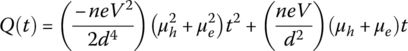
where V is the applied voltage and μe and μh are the mobilities of electrons and holes, respectively. The drift times of charge carriers are given by

The shape of current pulse can be obtained by differentiating the charge pulse in respect to time:

The shapes of charge and current pulses from a transmission detector are schematically shown in Figure 1.35.

Figure 1.35 Current and charge pulses from a transmission silicon detector.
When silicon detectors are used for detecting charged particles stopping in the detector, the electric field sensed by the charge carriers can be complicated due to several effects. One important effect resulted from the fact that for heavy charged particles such as alpha particles and fission fragments, the density of electron–hole pairs is high to form a plasma‐like cloud of charge. Consequently, while the outer region of the charge cloud senses the external electric field, the interior of the charge cloud is shielded from the influence of the electric field. As the charge carriers at the outer edge of the cloud move away, the charges at the interior become subject to the applied field and begin to drift. This process introduces a delay in the drift of charge carriers, which is called plasma time (Tp). As a result of this delay, the charge collection time in the detector increases and the shape of the pulse is modified. Even in the absence of the plasma effect, the time needed for the charge carriers to travel to the electrodes (Tr) is dependent on the particle’s range in the detector. Since both Tp and Tr depend on the ionization density or the ion number (Z) of the incident ion, the shape of the pulses will be dependent upon the type of charged particle, and thus one can determine the type of the particle by analyzing the shape of the pulses [58, 59].
1.3.2.3 Compound Semiconductor Detectors
Although germanium and silicon have proven to be useful and important semiconductor detector materials, their use for an increasing range of applications is becoming marginalized by their modest stopping powers and/or their need for ancillary cooling systems. On the other hand, compound semiconductor detectors can be operated at room temperature (bandgap energies >1.35 eV) and exhibit higher quantum efficiency than silicon and germanium due to their high atomic number and mass density. However, the problems regarding crystal growth defects and impurities are far more problematic for this group of detectors. Consequently, due to much higher density of traps than in the elemental semiconductors, these detectors suffer from short lifetimes for charge carriers, which can limit the performance of the detectors. In spite of these limitations, compound semiconductors such as cadmium telluride (CdTe), cadmium zinc telluride (CdZnTe), mercuric iodide (HgI2), and thallium bromide (TlBr) have been under extensive research, and commercial devices have been developed for medical and industrial applications. In the following, we will discuss the pulses from some of the common compound semiconductor detector configurations. More details on compound semiconductor detectors can be found in Refs. [32, 60].
1.3.2.3.1 Planar Geometry
The simplest form of a compound semiconductor detector is in planar geometry where the semiconductor material is sandwiched between two planar metal electrodes. If a uniform electric field is assumed in the detector, the absolute current induced on the electrodes by the drift of electrons and holes liberated in an interaction is given by the Shockley–Ramo theorem as
where e is the electron charge, d is the detector thickness and ve and vh are the drift velocities of electrons and holes and n(t) represents their corresponding concentrations at instant t. By taking into account the trapping effects, the numbers of drifting electrons and holes as a function of time are given by
where n∘ is the initial number of electron–hole pairs and τe and τh are lifetimes of electrons and holes. By combining Eqs. 1.85 and 1.86 and the approximate linear relation of the drift velocities and applied electric field, the time‐dependent induced charge on the electrodes is obtained by

where V is the applied voltage and μe and μh are, respectively, the mobilities of electrons and holes. The charge carriers contribute to the charge induction during their transit times, which are given by
where x∘ represents the location of gamma‐ray interaction in the detector, measured from the cathode, and the e and h subscripts represent electrons and holes, respectively. The total induced charge after the charge collection time is calculated as

This equation is called the Hecht equation and reflects the effects of charge transport parameters on the total collected charge [61]. Figure 1.36 shows the shape of charge pulses calculated for different interaction points in a 1 mm thick CdTe detector. As a result of a significant difference in the drift velocity of electrons and holes, the charge collection time strongly depends on the interaction location of gamma rays, and due to the charge trapping effect, the total induced charge is smaller than the amount of initial ionization. In particular, a significant amount of charge loss happens for interactions close to the anode, where holes need to drift all the distance between the electrodes with their small drift mobility and short lifetime.

Figure 1.36 Schematic of a simple planar compound semiconductor detector and charge pulses calculated for various interaction points in a 1 mm thick CdTe detector.
The aforementioned description of pulses is valid under the assumption that the electric field inside the detector is uniform. However, studies on the electric field distribution show that in some of the compound semiconductor detectors such as CdTe, this assumption is not valid [62]. The nonuniform electric field may be a consequence of different phenomena such as space‐charge polarization [63]. Polarization is a consequence of strong carrier trapping by deep impurity levels. As a result of charge trapping, a space‐charge region with a high charge density can be created, which causes a significant change in the profile of the internal electric field. This leads to some deviations from calculated pulses, but the equations are still good approximations for describing the shape of pulses from planar detector. In addition to electric field nonuniformities, detectors may also show some de‐trapping effects. The de‐trapping effect happens when trapped charges are released from the trap by thermal excitations. According to a formalism for including trapping and de‐trapping effects in CdTe detectors, the induced charge due the charge carrier i for times smaller than the charge collection time is given by [64, 65]

with

where i represents electrons or holes, TR is the charge collection time of the charge carrier i, and τ and τd are the trapping and de‐trapping times of the carriers, respectively. The expression for the charge pulse for times greater than charge collection times (t > TR) is very complicated and requires computer simulations [65]. The shapes of pulses with and without including the de‐trapping effects are schematically shown in Figure 1.37.

Figure 1.37 A schematic illustration of charge pulses with and without charge trapping and de‐trapping effects.
In Section 1.3.2.2 we discussed the use of silicon detectors as ΔE detector. Detectors with charge trapping effects are also sometimes used as transmission charged particle detector. A detector made of diamond is the main example of such detectors though diamond is not a compound semiconductor material. The shape of pulses in such detectors can be obtained by integrating the charge induced by point‐like ionizations. A description of pulses from transmission detectors in the presence of charge trapping effects can be found in Ref. [66].
1.3.2.3.2 Single‐Polarity Charge Sensing
In compound semiconductor detectors with planar geometry, the charge trapping effect makes the total induced charge dependent on the interaction location of gamma rays. Consequently, as a result of the random locations of gamma‐ray interactions, fluctuations in the amount of collected charges result that can significantly degrade the performance of the detectors. The charge trapping effect is particularly serious for holes due to their shorter lifetimes and small mobility. For example, in CdZnTe grown by the high‐pressure Bridgman technique, typical lifetimes are τe = 3 × 10⁻⁶ s and th < 0.5 × 10⁻⁶ s, while the drift velocity of holes is almost 10 times smaller than that of electrons. The problems of hole trapping limit the useful thickness of planar detectors to a few millimeters, which is obviously insufficient for many applications involving energetic gamma rays. In order to overcome the effect of severe trapping of holes in wide bandgap semiconductors, single‐polarity charge sensing techniques have been proposed in which the pulse amplitude is sensitive only to the electrons and not the holes as dictated by the distribution of weighting field. The earliest single‐polarity charge sensing technique implemented on semiconductor gamma‐ray detectors was the development of hemispherical devices [67]: a small dot anode was placed in the focus of the hemispheric cathode electrode, and the signal was read out from the small‐area anode. Because of the small area of the anode relative to the cathode, the weighting potential is very low within most volume of the detector and rises rapidly to 1 near the anode electrode. Therefore, the induced charge on the anode is dominated by the movement of charge carriers near the anode. These charge carriers for the majority of gamma‐ray interactions are electrons because holes drift toward the negative electrode, and therefore the contribution of holes in the induced signal is reduced. The performance of this detector is limited by a very weak electric field near the cathode where electrons move very slowly, and thus severe charge trapping can occur.
A very effective single‐polarity charge sensing technique is the coplanar structure. The coplanar structure is essentially an evolution of the classical gridded ionization chamber (see Section 1.3.1.2) and was first implemented on semiconductor detectors by Luke in 1994 [68]. The concept of a coplanar detector is illustrated in Figure 1.38a. In this detector structure, instead of a single electrode on the anode, parallel strip electrodes are used, and the strips are connected in an alternate manner to give two sets of grid electrodes. A voltage difference between these two sets of electrodes is applied so that the electrons are always collected by one electrode, called collecting electrode. The other electrode is called non‐collecting electrode. The weighting potentials (or induced charge) of the collecting electrode and non‐collecting electrode are schematically shown in Figure 1.38b. The characteristic shape of these weighting potentials reflects the fact that the induced charges on both anode electrodes initially increase identically due to the symmetry between the two set of anodes, but when electrons move closer to the anode surface, this regime is followed by a rapid increase of the weighting potential of the collecting electrode and a drop to zero for the non‐collecting electrodes [69]. Single‐polarity charge sensing is implemented by reading out the difference signal between the collecting and non‐collecting electrode. If the trapping of electrons is negligible, the amplitude of the differential signal is independent of the depth of the gamma‐ray interaction, while the contribution of holes is eliminated. Another single‐polarity charge sensing method was achieved based on the use of the electrode structure of a silicon drift detector (see Figure 1.34) on compound semiconductors [70]. The electric field formed by a set of focusing electrodes drives the electrons to a small anode where they are collected. The weighting potential of the small anode, calculated by applying a unit potential on the anode and zero on all other electrodes, has very low value in most of the volume of the detector and sharply rises to 1 in the immediate vicinity of the small anode. This shape results from the small dimension of the collecting anode and the closeness of the nearest focusing electrode to the collecting anode. Because the nearest focusing electrode forces the weighting potential of the collecting anode to be zero very close to the collecting anode, the induced charge on the small anode is dominated by the number of electrons collected, and the contribution of holes is suppressed.

Figure 1.38 (a) The structure of a coplanar detector. (b) The weighting potentials of the collecting and non‐collecting anode electrodes.
1.3.2.3.3 Pixel and Strip Geometries
Planar detectors with strip and pixel electrodes are widely used for radiation imaging applications. By reading out the signals from individual pixels or strips of a properly segmented detector, high resolution position measurements can be achieved as required in applications such as medical and industrial imaging. Although pixel and strip electrodes were first developed for two‐dimensional position sensing [71, 72], it was later realized that single‐polarity charge sensing can also be achieved by reading out signals from individual pixel or strip electrodes [73, 74]. For pixel detectors, it has been shown that the deleterious effects of hole trapping can be greatly reduced if the pixel dimension, w, is made small relative to the detector thickness, d [74]. This effect is generally referred to as the small pixel effect. Figure 1.39 shows a cross‐sectional view of a pixel detector and typical plots of weighting potential along the center of a pixel. The details of the calculation of weighting potentials in pixel detectors can be found in several references [74, 75]. It is seen that the weighting potential that surrounds a small pixel is only of considerable magnitude close to the pixel. Therefore charge carriers will only induce a significant signal on a pixel when they are in close proximity to the pixel, which means that the holes drifting toward the cathode will not induce a significant signal on the pixel. As the signal is induced by electrons drifting near to the pixels, as opposed to drifting through the entire bulk of the material, the signals from small pixel detectors will have a faster signal risetime than planar detectors. In a strip detector also the small size of a strip electrode and the presence of closely spaced adjacent electrodes result in a strong peaked weighting potential distribution near the strips, while the weighting potential is very low in most of the detector volume. Therefore, the charge induction is mainly due to the drift of electrons, and the contribution of holes is suppressed. In both strip and pixel detectors, to achieve the best charge collection performance, the dimension of the electrodes needs to be specifically designed to match the material characteristics and operating conditions of the detector, though the electrode dimensions required for optimal charge collection may not coincide with the required imaging.

Figure 1.39 A pixel detector and a typical plot of the weighting potential along the z‐axis through the middle of the pixel.
1.4 Scintillation Detectors
1.4.1 Principles
In scintillation detectors radiation detection is accomplished by the use of a scintillator material: a substance that emits light when struck by an ionizing particle. The scintillations emitted from the scintillator are then converted to an electrical signal by means of a photodetector. The scintillator materials are available as solid, liquid, or gas, but they can be broadly categorized into organic and inorganic scintillators. The important difference between the two groups of scintillators is that organic scintillators are composed of low atomic number elements and, therefore, are more suitable for neutron and charged particle detection, while inorganic scintillators normally contain a large fraction of atoms with a high atomic number and, therefore, are suitable for gamma‐ray detections. The physics of the scintillation mechanism in organic and inorganic scintillating materials is, however, very different. In the following sections we will briefly discuss the scintillation mechanism in organic and inorganic scintillators.
1.4.2 Inorganic Scintillators
In inorganic scintillators, the scintillation mechanism depends on the structure of the crystal lattice. In a pure inorganic crystal lattice, electrons are only allowed to occupy the valance or conduction band. Electrons that are bound at the lattice sites are in the valance band, while electrons in the conduction band have sufficient energy to freely migrate throughout the crystal. The forbidden band or bandgap is the range of energies in which electrons can never be found in the pure crystal. When an ionizing radiation interacts with an inorganic scintillator crystal, a large number of electron–hole pairs are created. The absorption of energy can elevate electrons from the valence band to the conduction band, leaving a hole in the valence band. The return of an electron to the valence band leads to the emission of a de‐excitation photon. The efficiency of light emission can be significantly increased by adding a small amount of impurities, called activators, to the crystal. Figure 1.40 shows the energy band structure of an activated crystalline scintillator. The activator creates special sites in the lattice at which the bandgap structure is modified. As a result, energy states are created within what would be the forbidden band in the pure crystal. The electron can de‐excite through these levels back to the valence band. Since the energy levels created by the activator’s presence within the crystal are narrower than in the pure crystal, the photons emitted by the transitions of electrons from upper to lower states will be lower in energy than in the pure crystal, and therefore the emission spectrum is shifted to longer wavelengths and will not be influenced by the optical absorption band of the bulk crystal. The main properties of a scintillator are scintillation efficiency, light output, emission spectrum, and decay time of scintillation light. The scintillation efficiency is defined as the ratio of the energy of the emitted photons to the total absorbed energy, and the light output is measured as the number of photons per MeV of energy absorbed in the detector. Some of the common inorganic scintillators are alkali‐halide scintillators such as thallium‐doped sodium iodide (NaI(Tl)) and cesium iodide (CsI(Tl)), non‐alkali scintillators such as barium fluoride (BaF2) and Bi4Ge3O12 (BGO), the rare‐earth halide family such as lanthanum bromide (LaBr3(Ce)), and so on. A review of the properties of different inorganic scintillators can be found in Ref. [76].

Figure 1.40 Energy bands in an activated crystalline inorganic scintillator.
1.4.3 Organic Scintillators
The scintillation mechanism in organic materials arises from transitions in the energy levels of a single molecule, and therefore organic scintillators can be found independently of the physical state. In practice, organic scintillators are used in the form of pure crystals, mixture of one or more compounds as liquids or plastics. These materials contain planar molecules built up mainly from condensed or linked benzenoid rings. A typical diagram of energy levels for these molecules is shown in Figure 1.41. When a charged particle passes through, kinetic energy is absorbed by the molecules, and electrons are excited to the upper energy levels. An excited electron can occupy a singlet excited state (system spin 0) or a triplet excited state (system spin 1). Associated with each electronic energy level, there is a fine structure that corresponds to excited vibrational modes of the molecule. The energy spacing between electron levels is on the order of a few electronvolts, while that between vibrational levels is of the order of a few tenths of electronvolts. The ground state is a singlet state, which is denoted by S00. The singlet excitations (S2, S3, etc,) generally decay immediately (<10 ps) to S1 electron state without the emission of light (internal conversion). From S10, there is generally a high probability of making a radiative decay to one of the vibrational states of ground state (S0). This process of light emission is described as the fluorescence or prompt component of scintillation light and is characterized with a decay time constant τ. In most organic scintillators, τ is the order of a few nanoseconds; therefore organic scintillators are fast detectors. The fact that S10 decays to excited vibrational states of S0, with the emission of radiation energy less than that required for the transition S00 to S1, also explains the transparency of the scintillators to their own radiation. For the triplet excited states, a similar internal degradation process occurs, which brings the system to the lowest triplet state (T0). While transitions from T0 to S0 are possible, they are, however, highly forbidden by multipole selection rules. The T1 state instead decays mainly by interacting with another excited T1 molecule through a process called triplet annihilation:

Figure 1.41 Schematic energy level diagram for an inorganic scintillator molecule. The upward pointing arrow refers to excitations, the downward pointing dashed arrow refers to decay without scintillation, and solid downward arrows refer to light emission.
This process leaves one of the molecules in S1 state. Radiation is then emitted by the S1 state as described for singlet states. This light comes after a delay time characteristic of the interaction between excited molecules and is called the delayed or slow component of the scintillator light. A very useful property of organic scintillators is that the intensity of the slow component depends on the specific ionization of charged particles, which enables one to differentiate between different kinds of particles by analyzing the shape of light pulses. This is called pulse‐shape discrimination and is a widely used technique for discriminating between different particles with plastic, liquid, and crystalline scintillators [77, 78].
1.4.4 The Time Evolution of Light Pulses
The time evolution of the light emission from scintillators, that is, the shape of light pulses, is described by the probability distribution function of scintillation photons emission in the course of a scintillation. This function describes the average shape of light pulses, and the output pulse for any individual scintillation will differ from the smooth average curve by the statistical fluctuations in the emission of photons. In most of the inorganic scintillation detectors, the average time evolution of the light emission process may be described as a simple exponential decay: the intensity of the light emission rises instantaneously to a maximum value at t = 0 and decay exponentially with decay time constant τ as
where I(t) is the intensity of the emission in photons per second and I(0) is the intensity at t = 0. This relation shows that the decay time constant should be as short as possible when counting rate of the detector is high. The total number of emitted photons (N) is obtained as
Then the emission of photons can be described as
In applications such as fast pulse timing, the approximation of the instant rise of the light output is not sufficient, and a finite risetime for the pulses should be considered. The risetime in inorganic scintillators is due to a complex sequence of events such as generation of primary electron–hole pairs by the incident particles, generation of electron–holes by energetic electrons, thermalization of electron–hole pairs, and creation of excitation and transfer to luminescent centers. In such cases, if the scintillator decays with a single decay time constant τ, then the light pulse can be described as

where τR is the time constant describing the population of optical levels. In many scintillators, two or more decay time constants are detected. For such scintillators, the time evolution of light pulse (with instant risetime) can be described as

where Nph is the total number of photons that are emitted with decay time constant τi. For many scintillators, two decay time constants are sufficient to describe the shape of the light pulses. One of the time constants is generally faster than the other, so it has become customary to refer them as fast and slow components or prompt and delayed components. In the case of organic scintillators, a unitary organic scintillator such as crystal, which is transparent to its own fluorescence, can be described by a single exponential decay function. In binary liquid scintillators, the light pulse is described by a fast and slow component like what was described before, and this model is widely used for describing the pulse‐shape discrimination property of the detectors. Most of the time an instant risetime is considered, but more realistic approximation of light pulse may be given by a convolution of a Gaussian function describing the population of optical levels with an exponentially decaying function. In all scintillators the observed shape of light pulse can be affected by the geometry of scintillator, boundary conditions, reflections, reemissions processes, and so on.
1.4.5 Photomultiplier Tubes
1.4.5.1 Principles
The scintillation light pulses from all types of scintillators should be converted to an electrical signal by using a photodetector. Photodetectors such as photomultiplier tubes (PMTs) have been widely used for this task due to several advantages such as high gain (up to 109). The light pulses obtained from scintillators are usually very weak, often less than a few 100 photons, and therefore the large gain of PMTs enables to obtain a detectable signal even with a few photons. PMTs also have exceptionally low noise, a wide bandwidth (up to 1 GHz), zero offset, and low and constant output capacitance.
A schematic representation of a PMT is shown in Figure 1.42. A PMT is typically constructed with an evacuated glass housing, containing a photocathode, an electron multiplier, and an anode. When light photons strike the photocathode, electrons are ejected from the surface of the photocathode as a consequence of the photoelectric effect. By an accelerating electric field, the ejected electrons move toward the electron multiplier where electrons are multiplied by the process of secondary emission. The electron multiplier consists of a number of electrodes called dynodes. Each dynode is held at a more positive potential than the preceding one. Upon striking the first dynode, more low energy electrons are emitted, and these electrons are in turn accelerated toward the second dynode. The geometry of the dynode chain is such that a cascade occurs with an exponentially increasing number of electrons being produced at each stage. Therefore, finally a large number of electrons reach the anode, which results in a sharp current pulse. Electric pulses can be also extracted from a dynode by using a suitable decoupling capacitor. The pulse induced on the anode is negative as electrons arrive to the anode, but the pulse from a dynode has positive polarity because electrons leave a dynode. The multiplication factor for a single dynode is defined as the ratio of the number of emitted secondary electrons to the number of incident electrons. The multiplication factor is a function of voltage difference between the dynodes and can be described as
where δ is the multiplication factor, Vd is the voltage difference between the dynodes, and K is a proportionality constant. If the applied voltage difference between the successive dynodes is constant, the overall gain of PMT is given by
where n is the number of dynodes. This relation indicates that the gain of a PMT is critically dependent on the applied voltages, and thus highly regulated voltage supplies are required to maintain a constant gain.

Figure 1.42 Schematic representation of a photomultiplier tube and its operation.
1.4.5.2 Voltage Dividers and Gain Stabilization
The acceleration of electrons toward the successive dynodes requires an electrostatic field between the dynodes, which is produced by applying voltage differences between the dynodes. The voltage differences between the successive dynodes are maintained by means of a voltage divider circuit. The common type of a voltage divider circuit consists of series‐connected resistors as illustrated in Figure 1.43. The chain of resistors divides the applied voltage in such a way that the photocathode is always negative with respect to the anode. This can be achieved by using a positive‐polarity voltage supply where the cathode is grounded and the anode is at high positive potential or by using a negative‐polarity voltage supply where the anode is grounded and the cathode is at high negative potential. The advantage of the negative‐polarity voltage supply is the elimination of pulse decoupling capacitor, which may be desirable for fast pulse timing applications. The choice of equal resistor values leads to the same voltage difference between all successive dynodes, which provides the highest gain for a given supply voltage and is generally suitable for nuclear spectrometry applications, but alternative voltage distributions can be also used to optimize the time characteristics while providing acceptable gain and linearity.

Figure 1.43 Schematic diagrams of a resistor chain voltage divider circuit.
In Figure 1.43, It represents the total electron current flowing through the divider and electron multiplier, and Ib represents the electron current drawn by the voltage divider with no light on the photocathode. This current is called the bleeder current and is simply given by the ratio of the applied high voltage and summed resistance of all the resistors. The current flowing through the electron multiplier is composed of the interstage currents i1, i2, and so on. If the interstage currents are negligible compared with the bleeder current, dynode potentials are maintained at a nearly constant value during the pulse duration. However, maintaining the bleeder current sufficiently large compared with the interstage current pulses is practically limited by large power consumption and heat dissipation in the divider resistors. When the interstage currents are not negligible, the current through the resistor x is It − ix, which consequently reduces the corresponding interelectrode voltage. To minimize the effect of peak interstage current on the dynode voltages, stabilizing capacitors are connected to the last few dynodes where peak currents are at a maximum. There are two methods of using the stabilizing capacitors: series connection method and parallel connection method [79, 80]. The use of series‐connected stabilizing capacitors is shown in Figure 1.44. In the absence of light pulses, the stabilizing capacitors are charged with the bleeder current, and in the presence of pulses, they act as local reservoirs of charge to help maintain the voltage on the dynodes. The capacitor values depend upon the value of the output charge associated with the pulse or train of pulses. The value of the final‐dynode‐to‐anode capacitor C is generally given by
where C is in farads, q is the total anode charge per pulse in coulombs, and Vd is the voltage across the capacitor. The factor 100 is used to limit the voltage change across the capacitor to a 1% maximum during a pulse. Capacitor values for preceding stages should take into account the smaller values of dynode currents in these stages, and normally a factor of 2 per stage is used. Dynode stages at which the peak current is less than 10% of the average current through the voltage divider do not require capacitors. For pulse durations in the 1–100 ns range, consideration should be given to the inherent stage‐to‐stage capacitances, which are on the order of 1–3 pF [79].

Figure 1.44 The use of stabilizing capacitors in a voltage divider with negative polarity.
In the high rate applications, it becomes difficult to maintain the stability of dynode voltages with a simple resistor and capacitor chain, and thus a variety of techniques have been proposed to maintain a constant gain for PMTs. Some of these techniques are reviewed in Refs. [79–82]. In one of the methods, Zener diodes are used in place of the resistors for the last few stages. A Zener diode maintains a constant voltage for currents above a minimum threshold, and thus the interstage voltages are maintained at constant voltage regardless of the supply voltage. Capacitors are also used in parallel to the Zener diodes to minimize the effect of noise generated by the Zener diode. A problem associated with the use of Zener diodes is that the fixed breakdown voltage of a Zener diode does not adjust to changes in power supply voltage, and thus, the voltage distribution among the electrodes may become highly imbalanced when the high voltage supply output level is greatly varied. The stabilization of a PMT gain can be also performed by using transistors in place of the voltage divider resistors at the latter stages. The transistors are connected in a modified emitter‐follower configuration and serve as buffers to regulate the voltage difference between the collector and emitter of each transistor across the corresponding pair of electrodes. Another approach for stabilizing PMT voltages is to use a small Cockcroft–Walton voltage multiplier circuit as shown in Figure 1.45. In this approach, an array of diodes is connected in series, and capacitors are connected in series along each side of the alternate connection points. If the voltage V is applied at the input, the circuit provides voltage potentials of 2 V, 3 V, and so on at each connection point, which are then used to maintain the interstage voltages. An important advantage of this circuit is its low power consumption, making it suitable for compact circuits.

Figure 1.45 A schematic representation of Cockcroft–Walton voltage divider.
1.4.5.3 The PMT Equivalent Circuit and Output Waveforms
The shape of the voltage pulse at the output of a PMT depends on the scintillation pulse, PMT characteristics, and conditions at the readout. If we assume the scintillation pulse has a shape described with Eq. 1.93, then the rate of electron emission from the photocathode exhibits the same time dependence:
where n is the number of photoelectrons. Due to the variations in the time of flights of the secondary electrons in the electron multiplier, the emission of even one single photoelectron leads to a cloud of secondary electrons with a finite space spread, thus resulting in an anode current pulse i∘(t) of finite duration. The current pulse i∘(t) is delayed against the radiation interaction by the total propagation time between the photocathode to the anode, which is constant for a given operating condition. The particular shape of the single electron pulse i∘(t) depends on the actual dynode geometry, but it can be approximated by a Gaussian function as [83]
where G is the PMT gain, tp is a constant representing the spread in electrons transit time, and e is the electron charge. The anode current pulse for a radiation interaction is composed of the overlap of several single electron pulses, and therefore, in general, it is represented by the convolution of Eqs. 1.99 and 1.100. However, if the spread in the transit time is small compared with the decay time constant of the scintillator, then the shape of the current pulse essentially follows the shape of scintillation light pulse and a faithful description of the current pulse induced on the anode can be given by
This current pulse is converted to a voltage pulse by a load resistor that connects the anode to the ground. The presence of load resistor is also necessary to avoid the anode charging up to a high voltage when the output is disconnected. Figure 1.46 shows the equivalent circuit of a PMT output when connected to a readout circuit. The anode resistor is R∘ and PMT is represented the capacitor C∘, which is the capacitance between the anode and ground, and its magnitude depends primarily on the area of the dynodes and on their spacing. The capacitance C1 is due to the cable, stray capacitance, and input capacitance of the readout circuit, and R1 represents the input resistance of the readout circuit. The combination of the resistors and capacitors in Figure 1.46 leads to an equivalent RC circuit where R = R∘‖R1, C = C1 + C∘, and τ1 = RC represents the time constant of the circuit. The voltage developed across the resistor is obtained by feeding the current pulse of Eq. 1.101 into the equivalent RC circuit as

Figure 1.46 The equivalent circuit for a PMT readout. A PMT is shown as a current generator.
For the choice of τ = τ1 = RC, we must take the limit τ → τ1 to obtain the corresponding expression. The shape of output anode voltage pulse varies with the time constant of the anode circuit. Figure 1.47 shows the shape of pulses for various time constants. If the time constant of the anode circuit is large compared with the decay time constant of the scintillator, then the anode current pulse is integrated by the RC circuit to produce a voltage pulse with amplitude GN∘e/C, which is proportional to the energy deposited in the scintillator material. Such integrating circuit is ideal for energy measurements, but long time constants obviously restrict the rate at which events can be handled. Moreover, the output is no longer a faithful reproduction of the input current. The use of very large values of load resistance creates the problems of deterioration of frequency response and output linearity, and the use of large capacitances causes loss in amplitude together with distortion of the input signal waveform. If the anode circuit time constant is much smaller than the decay time constant of the scintillator, then a faster pulse with a faithful reproduction of the decay time constant of scintillation light pulse is achieved, which is favorable in timing and pulse‐shape discrimination applications.

Figure 1.47 PMT output voltage pulses for different circuit time constants.
1.4.6 Semiconductor Photodetectors
In spite of various advantages, PMTs have several handicaps: they are sensitive to magnetic fields, their price is high, and they are bulky. Moreover, PMTs require a very high supply voltage in the range of kilovolts and their power consumption is large. To overcome these shortcomings, silicon photodetectors have been under development to replace PMTs in applications such as medical imaging. In the following, we review some of the basic properties of silicon photodetectors such as photodiodes, avalanche photodiodes (APDs), and silicon photomultipliers (SiPMs) [84].
1.4.6.1 Photodiodes
The light detection in photodiodes is based on the creation of electron–hole pairs in the depleted region of a p–n junction. The energy of light photons should be sufficiently high to bring the electrons above the energy bandgap of the semiconductor, which in the case of silicon is 1.12 eV corresponding to the wavelength below 1100 nm. The electron–hole pairs then drift toward the electrodes and a signal is induced on the electrodes. The depth of the depletion region must be thick enough to achieve sufficient sensitivity. The mean free path of optical photons in silicon varies from 0.1 µm at 400 nm to 5 µm at 700 nm. On the other side, a too thick depletion region may lead to large thermally generated noise and poor timing performance. Silicon photodiodes are also built with pin structure where an intrinsic layer is placed between the p and n sides of the diode to increase the sensitive volume. In general, silicon photodiodes are not expensive if the detector area is small, are insensitive to magnetic fields, and have excellent quantum efficiency. However, photodiodes have no internal amplification of the signal, so the number of charges in the signal equals the number of detected photons. This limits these devices to applications where large numbers of photons are produced.
1.4.6.2 Avalanche Photodiodes
An APD is a silicon photodiode with internal gain. If the electric field in the silicon is high enough, primary charge carriers can produce new pairs by impact ionization. The increase in the number of charge carriers leads to stronger output signals compared with simple photodiodes. Avalanche multiplication is a statistical process and leads to a fluctuation in the signal, which is called the excess noise. In the avalanche multiplication process, the ionization rate is higher for electrons than for holes, so the amplification process for electrons starts at lower fields and the avalanche grows in the direction of electron movement. At high electric fields, holes also start to ionize, but when the ionization probability is high, the amplification can no longer be controlled. Therefore, for stable avalanche multiplication, it is essential that only one type of charges is multiplied and the other type being only collected. Three main structures of have been used for APDs including beveled‐edge, reverse, and reach‐through diodes [85, 86]. The structure of a reach‐through APD is shown in Figure 1.48. The electric field consists of a low electric field region, where the photons convert into electron–hole pairs, followed by a high field region, where the field is sufficient to cause electron multiplication. The electric field distribution is produced by a suitable doping profile and allows only for the multiplication of electrons. For a long time, APDs were limited to very small sensitive areas, had a large dark current, and were expensive and unreliable. During the past years, the technology to produce APDs has improved dramatically, and it is now possible to obtain APDs with large area, low capacitance, low lark current, high gain, high quantum efficiency, and stable operation. However, APDs are not still suitable for weak light pulses, and their operation requires accurate control of both temperature and bias voltage.

Figure 1.48 Schematic structure of a reach‐through APD and its electric field distribution. π represents either lightly doped p‐type material or intrinsic material.
1.4.6.3 Silicon Photomultipliers (SiPMs)
In spite of internal gain, an APD still needs some 20 photons for a detectable output pulse. An SiPM is a silicon device that can detect single photons like a vacuum PMT. This device is also sometimes referred to as multi‐pixel photon counter (MPPC) or pixellized photodetector (PPD) [87, 88]. Its structure consists of several miniaturized photodiodes belonging to the same silicon substrate. The photodiodes are connected in parallel, so the output of the device is the sum of the photodiodes’ outputs. The photodiodes are designed to operate in the Geiger region, which makes them sensitive to single photons. A resistor is connected in series to each photodiode by which the photodiode operation in Geiger mode is quenched. Each photodiode with its quenching resistor is called a microcell whose operation in Geiger mode can be explained with reference to Figure 1.49 as follows: the photodiode has a breakdown voltage (Vbr) at which the current flow in the photodiode significantly increases. For operation in Geiger mode, a bias voltage (Vbias) in excess of Vbr is applied. The difference between the bias voltage and breakdown voltage is called overvoltage value. Initially, on application of Vbias, no current flows in the photosensitive region of the photodiode but a negligible parasitic current. On arrival of a photon and conversion of the photon into an electron–hole pair, the charge carriers undergo impact ionization, leading to avalanche multiplication. During the avalanche process, the photodiode current significantly increases; thus the voltage drop across the resistor causes the photodiode voltage and electric field to decrease and the avalanche is quenched. When the current returns to its initial value, the voltage bias across the photodiode increases to the original Vbias, and the photodiode returns to a state that can detect the next photon. The gain of a single microcell is given by the overvoltage and the capacitance of the cell (C) as [89]

Figure 1.49 The operation of a single photodiode in Geiger mode.
The capacitance of the microcell is given by the sum of the photodiode capacitance and the parasitic capacitance of the resistor and e is the electric charge. This gain is in the range of 105–107.
A commercial SiPM can have from hundreds to thousands of microcells connected in parallel as shown in Figure 1.50a. When one of the microcells undergoes a Geiger discharge, the SiPM can be modeled with the circuit shown in Figure 1.50b [90]. Rq represents the quenching resistor with its parasitic capacitance Cq, Cd is the photodiode capacitance, Cg is the capacitances associated with the connection of microcells in parallel, and the current source models the current pulse produced in the Geiger discharge. Since the avalanche mechanism in the tiny photodiode is very fast, it is possible to model its contribution as a Dirac delta function for a photon absorbed in time t∘ as
where Q is the charge produced in the microcell given by the product of the microcell gain (G) and electric charge. When an SiPM is exposed to a light pulse from a scintillator, several microcells may undergo Geiger discharge, while the output signals of the microcells have the same shape and charge. In case of not too intense light pulses, the number of fired microcells is in first order proportional to the number of photons, but for intense light pulses, saturation effects may set in. Summing up all microcell contributions along a reduced period of time (a few nanoseconds), the SiPM output current pulse is given by

Figure 1.50 A schematic representation of an SiPM and its equivalent circuit.
The output current is converted to a voltage pulse at the input of the readout circuit. Similar to the calculation of the output voltage pulse from a PMT, the output voltage can be calculated by taking into account the input resistance and capacitance of the readout circuit. However, this voltage value will be observable at amplifier output depending on its bandwidth and slew‐rate characteristics. Some calculations of output current pulses can be found in Ref. [91].
An important parameter of an SiPM is PDE, which is the efficiency at which photons of given wavelength can be detected. The PDE is the product of three factors. The first factor is the ratio of the sensitive area and total area of the SiPM. The sensitive area in SiPMs is smaller than the total area due to the presence of an optically inactive structure that contains the resistors and capacitors and also a dead space necessary to provide a physical separation for the individual microcells. The percentage of active area in an SiPM is termed the fill factor. The second factor is the quantum efficiency, defined as the probability that an electron–hole pair is generated by an incident photon. The third factor is the probability that an electron or hole initiates a Geiger discharge in the depletion region of a microcell. The noise in SiPM devices is mainly due to the dark count rate: an electron–hole pair can be thermally generated, triggering an avalanche in a microcell without an optical photon impinging on it. The dark noise rate depends on the working temperature and on the overvoltage, and it is directly proportional to the active area of the device. Another drawback of SiPM is afterpulses, which are produced by charges from the avalanche process that are temporarily trapped and produce a new avalanche after their release. The trapped charge carriers can have a lifetime from tens to hundreds of nanoseconds, and therefore a second Geiger discharge can be triggered after the complete microcell recharge, increasing artificially the number of counted events. Another unwanted feature of SiPM is cross talk, which occurs when the photon produced in the avalanche escapes from the microcell into a neighboring cell and induces a new Geiger discharge. The dynamic range of an SiPM can be defined as the optical signal level range over which the detector provides a useful output. This range extends from the lowest detectable signal level to the optical signal level that results in saturation effects in the output signal. The saturation is due to the fact that after a single microcell is fired and before the Geiger discharge is quenched, the microcell is blind to other photons, and therefore, the number of microcells sets an upper limit to the number of photons that can be simultaneously detected. If the light intensity is high, the output can completely saturate since no more microcells are available to detect incoming photons until some of the microcells have recovered from Geiger discharge. The recovery time increases with the photodiode area and the quench resistor and parasitic impedance. The fastest recovery times are achieved with the smallest microcell size, but at the expense of the fill factor. The dynamic range of an SiPM is therefore a function of the total number of microcells and the PDE of the device. To avoid saturation effects, the number of microcells has to be chosen depending on the expected number of photons. In the case of scintillation pulses, the number of photons depends on scintillation yield, but due to photons exponential time distribution, the saturation effect is less pronounced when the decay time constant of the scintillator is longer than the recovery time of the microcells.
References
- 1 C. Y. Fong and C. Kittel, Am. J. Phys. 35 (1967) 1091.
- 2 W. Shockley, J. Appl. Phys. 9 (1938) 635.
- 3 S. Ramo, Proceedings of the I.R.E., September, 1939, p. 584.
- 4 Z. He, Nucl. Instrum. Methods A 463 (2001) 250–267.
- 5 G. Cavalleri, et al., Nucl. Instrum. Methods 92 (1971) 137.
- 6 S. Ettenauer, Nucl. Instrum. Methods A 588 (2008) 380–383.
- 7 F. Sauli, Gaseous Radiation Detectors: Fundamentals and Applications, Cambridge University Press, Cambridge, 2014.
- 8 G. F. Knoll, Radiation Detection and Measurements, Forth Edition, John Wiley & Sons, Inc., New York, 2010.
- 9 H. Raether, Electron Avalanches and Breakdown in Gases, Butterworths, London, 1964.
- 10 C. Cernigoi, G. Pauli, and C. Poiani, Nucl. Instrum. Methods 2 (1958) 261–269.
- 11 M. Hagiwara, T. Sanami, T. Oishia, M. Baba, and M. Takada, Nucl. Instrum. Methods A 592 (2008) 73–79.
- 12 J. Hendrix and A. Lentfer, Nucl. Instrum. Methods A 252 (1986) 246–250.
- 13 J. E. Draper, Nucl. Instrum. Methods 30 (1964) 148–150.
- 14 W. Riegler, Nucl. Instrum. Methods A 491 (2002) 258–271.
- 15 V. Radeka, Annu. Rev. Nucl. Part. Sci. 38 (1988) 217–277.
- 16 S. R. Elliott, Nucl. Instrum. Methods A 290 (1990) 158–166.
- 17 G. Charpak, J. Phys. 30 (1969) 86 C2.
- 18 G. Charpak and F. Sauli, Nucl. Instrum. Methods 162 (1979) 405–428.
- 19 J. R. Thompson, J. S. Gordon, and E. Mathieson, Nucl. Instrum. Methods A 234 (1985) 505–511.
- 20 F. Sauli and A. Sharma, Annu. Rev. Nucl. Part. Sci. 49 (1999) 341.
- 21 A. Oed, Nucl. Instrum. Methods A 263 (1988) 351.
- 22 F. Sauli, Nucl. Instrum. Methods A 386 (1997) 531.
- 23 Y. Giomataris, et al., Nucl. Instrum. Methods A 376 (1996) 29.
- 24 F. Sauli, Nucl. Instrum. Methods 805 (2016) 2.
- 25 S. Bachmann, et al., Nucl. Instrum. Methods A 479 (2002) 294.
- 26 G. Charpak, J. Derré, Y. Giomataris, and Ph. Rebourgeard, Nucl. Instrum. Methods A 478 (2002) 26.
- 27 D. H. Wilkinson, Nucl. Instrum. Methods 321 (1992) 195–210.
- 28 D. H. Wilkinson, Nucl. Instrum. Methods 383 (1996) 516–522.
- 29 D. H. Wilkinson, Nucl. Instrum. Methods 383 (1996) 523–527.
- 30 D. H. Wilkinson, Nucl. Instrum. Methods 435 (1999) 446–455.
- 31 F. S. Goulding, Nucl. Instrum. Methods 43 (1966) 1–54.
- 32 A. Owens, Compound Semiconductor Radiation Detectors, CRC Press, Boca Raton, 2012.
- 33 J. Eberth and J. Simpson, Prog. Part. Nucl. Phys. 60 (2008) 283–337.
- 34 R. J. Cooper, D. C. Radford, P. A. Hausladen, and K. Lagergren, Nucl. Instrum. Methods A 665 (2011) 25–32.
- 35 A. S. Adekola, J. Colaresi, J. Douwen, W. F. Mueller, and K. M. Yocum, Nucl. Instrum. Methods A 784 (2015) 124–130.
- 36 J. Llacer, Nucl. Instrum. Methods 98 (1972) 259–268.
- 37 Th. Kroll, et al., Nucl. Instrum. Methods A 371 (1996) 489–496.
- 38 B. Philhour, et al., Nucl. Instrum. Methods A 403 (1998) 136.
- 39 J. H. Lee, H. S. Jung, H. Y. Cho, Y. K. Kwon, and C. S. Lee, IEEE Trans. Nucl. Sci. 57 (2010) 2631.
- 40 S. M. Sze, Physics of Semiconductor Devices, John Wiley & Sons, Inc., New York, 1981.
- 41 S. Akkoyun and A. Algora, Nucl. Instrum. Methods A 668 (2012) 26–58.
- 42 I. Mateu, P. Medina, J. P. Roques, and E. Jourdain, Nucl. Instrum. Methods A 735 (2014) 574–583.
- 43 Th. Kroll and D. Bazzacco, Nucl. Instrum. Methods A 463 (2001) 227–249.
- 44 K. Vetter, et al., Nucl. Instrum. Methods A 452 (2000) 223–238.
- 45 M. Amman and P. N. Luke, Nucl. Instrum. Methods A 452 (2000) 155.
- 46 N. Goel, et al., Nucl. Instrum. Methods A 700 (2013) 10–21.
- 47 S. J. Colosimo, et al., Nucl. Instrum. Methods A 773 (2015) 124.
- 48 R. A. Kroeger, et al., Nucl. Instrum. Methods A 422 (1999) 206–210.
- 49 E. Gatti, et al., Nucl. Instrum. Methods A 253 (1987) 393–399.
- 50 P. N. Luke, N. W. Madden, and F. S. Goulding, IEEE Trans. Nucl. Sci. NS‐32 (1985) 457.
- 51 E. H. M. Heijne, Nucl. Instrum. Methods 591 (2008) 6–13.
- 52 P. Rehak, IEEE Trans. Nucl. Sci. 51 (2004) 2492–2497.
- 53 C. Guazzoni, Nucl. Instrum. Methods 624 (2010) 247–254.
- 54 E. Gatti and P. F. Manferedi, Rivista Del Nuovo Cimento 9 (1986) 1.
- 55 M. Brigida and C. Favuzzi, Nucl. Instrum. Methods A 533 (2004) 322–343.
- 56 E. Gatti and P. Rehak, Nucl. Instrum. Methods A 541 (2005) 47–60.
- 57 J. Kemmer, Nucl. Instrum. Methods 169 (1980) 499.
- 58 J. B. A. England, G. M. Field, and T. R. Ophel, Nucl. Instrum. Methods A 280 (1989) 291–298.
- 59 Z. Sosin, Nucl. Instrum. Methods A 693 (2012) 170.
- 60 A. Owens and A. Peacock, Nucl. Instrum. Methods A 531 (2004) 18.
- 61 K. Hecht, Z. Phys. 77 (1932) 235.
- 62 A. A. Turturici, L. Abbene, G. Gerardi, and F. Principato, Nucl. Instrum. Methods A 795 (2015) 58–64.
- 63 K. Suzuki, T. Sawada, K. Imai, and S. Seto, IEEE Trans. Nucl. Sci. 59, 4, (2012) 1522.
- 64 W. Akutagawa and K. Zanio, J. Appl. Phys. 40 (1969) 3838.
- 65 M. Martini and T. A. McMath, Nucl. Instrum. Methods 79 (1970) 259.
- 66 M. Nakhostin, Nucl. Instrum. Methods A 703 (2013) 199.
- 67 K. Zanio, Rev. Phys. Appl. 12 (1977) 343.
- 68 P. N. Luke, Appl. Phys. Lett. 65 (1994) 2884.
- 69 Z. He, Nucl. Instrum. Methods A 365 (1995) 572–575.
- 70 B. E. Patt, et al., Nucl. Instrum. Methods A 380 (1996) 276.
- 71 F. P. Doty, et al., Nucl. Instrum. Methods A 353 (1994) 356.
- 72 J. M. Ryan, et al., Proc. SPIE 2518 (1995) 292.
- 73 J. A. Heanue, J. K. Brown, and B. H. Hasegawa, IEEE Trans. Nucl. Sci. 44 (1997) 701.
- 74 H. H. Barrett, et al., Phys. Rev. Lett. 75 (1995) 156.
- 75 A. Zumbiehl, et al., Nucl. Instrum. Methods A 469 (2001) 227–239.
- 76 M. J. Weber, JOL 100 (2002) 35–45.
- 77 F. D. Brooks, Nucl. Instrum. Methods 162 (1979) 477–505.
- 78 N. Zaitseva, et al., Nucl. Instrum. Methods A 668 (2012) 88–93.
- 79 R. W. Engstrom, Photomultiplier Handbook, Burle Technologies, Inc., Lancaster, 1980.
- 80 T. Hakamata, et al., Photomultiplier Tubes, Basics and Applications, Third Edition, Hamamatsu Photonics, K.K., Hamamatsu City, 2007.
- 81 A. Brunner, et al., Nucl. Instrum. Methods A 414 (1998) 466–476.
- 82 R. D. Hiebert and H. A. Thiessen, Nucl. Instrum. Methods 142 (1977) 467–469.
- 83 E. Kowalski, Nuclear Electronics, Springer Verlag, Berlin, New York, 1970.
- 84 S. Korpar, Nucl. Instrum. Methods A 639 (2011) 88–93.
- 85 M. Moszynski, et al., IEEE Trans. Nucl. Sci., 48, 4, (2001) 1205.
- 86 J. P. Pansart, Nucl. Instrum. Methods A 387 (1997) 186–193.
- 87 D. Renker, Nucl. Instrum. Methods A 567 (2006) 48–56.
- 88 P. Eckert, et al., Nucl. Instrum. Methods A 620 (2010) 217–226.
- 89 C. Piemonte, et al., IEEE Trans. Nucl. Sci. NS‐54 (2007) 236–244.
- 90 F. Corsi, et al., IEEE Nuclear Science Symposium Conference Record, 2006, pp. 1276–1280.
- 91 F. Corsi, et al., Nucl. Instrum. Methods A 572 (2007) 416–418.