
Chapter 2
Filtering and Querying a Table
IN THIS CHAPTER
![]() Understanding how to filter and query a table
Understanding how to filter and query a table
![]() Using AutoFilter to show only the data you want to see
Using AutoFilter to show only the data you want to see
![]() Filtering a table with custom criteria
Filtering a table with custom criteria
![]() Filtering a table on font color, fill color, or cell icons
Filtering a table on font color, fill color, or cell icons
![]() Using database functions to compute statistics from records that match your filter criteria
Using database functions to compute statistics from records that match your filter criteria
![]() Performing external data queries with text files, web pages, and data files kept in other database sources
Performing external data queries with text files, web pages, and data files kept in other database sources
It’s one thing to set up a table and load it with tons of data and quite another to get just the information that you need out of that table. How you go about extracting the data that’s important to you is the subject of this chapter. The process for specifying the subset of the data that you want displayed in an Excel table is called filtering the table. The process for extracting only the data that you want from the table is called querying the table.
Besides helping you with filtering and querying the data in your table, this chapter also explains how you can use Excel’s database functions to perform calculations on numeric fields for only the records that meet the criteria that you specify. These calculations can include getting the total (DSUM), the average (DAVERAGE), the record count (DCOUNT and DCOUNTA), and the like.
Finally, this chapter introduces you to querying an external data source to bring some or all of its data into the more familiar worksheet setting. Data sources can be in the form of external databases in other Windows database programs, such as Microsoft Access or in even more sophisticated, server-based database-management systems, such as those provided by SQL Server, Azure SQL Database, and ODBC connections. They can also be in the form of tables stored on web pages and in text files, which can be parsed into separate cells of an Excel worksheet.
Filtering Data
Filtering the table to leave behind only the information that you want to work with is exactly the procedure that you follow in Excel. At the most basic level, you use the AutoFilter feature to temporarily hide the display of unwanted records and leave behind only the records that you want to see. Much of the time, the capabilities of the AutoFilter feature are all that you need, especially when your main concern is displaying just the information of interest in the table.
You'll encounter situations, however, in which the AutoFilter feature isn't sufficient, and you must do what Microsoft refers to as advanced filtering in your table. You need to use advanced filtering when you use computed criteria (such as when you want to see all the records where the entry in the Sales column is twice the amount in the Owed column) and when you need to save a copy of the filtered data in a different part of the worksheet (Excel’s version of querying the data in a table).
Using AutoFilter
Excel’s AutoFilter feature makes filtering out unwanted data in a table as easy as clicking the AutoFilter button on the column on which you want to filter the data and then choosing the appropriate filtering criteria from that column’s drop-down menu.
 If you open a worksheet with a table and you don’t find AutoFilter buttons attached to each of the field names at the top of the list, you can display them by positioning the cell pointer in one of the cells with the field names and then clicking the Filter command button on the Ribbon’s Data tab or pressing Ctrl+Shift+L or Alt+AT.
The filter options on a column’s AutoFilter drop-down menu depend on the type of entries in the field. On the drop-down menu in a column that contains only date entries, the menu contains a Date Filters option to which a submenu of the actual filters is attached. On the drop-down menu in a column that contains only numeric entries (besides dates) or a mixture of dates with other types of numeric entries, the menu contains a Number Filters option. On the drop-down menu in a column that contains only text entries or a mixture of text, date, and other numeric entries, the menu contains a Text Filters option.
Doing basic filtering by selecting specific field entries
Besides the Date Filters, Text Filters, or Number Filters options (depending on the type of field), the AutoFilter drop-down menu for each field in the table contains a list box with a complete listing of the unique entries made in that column, each with its own check box. At the most basic level, you can filter the table by clearing the check box for all the entries whose records you don’t want to see in the list.
This kind of basic filtering works best in fields such as City, State, or Country, which contain many duplicates, so you can see a subset of the table that contains only the cities, states, or countries you want to work with at the time.
The easiest way to perform this basic type of filtering on a field is to first deselect the (Select All) check box at the top of the field’s list box, and then select each of the check boxes containing the entries for the records you do want displayed in the filtered table. After you finish selecting the check boxes for all the entries you want to keep, click OK to close the AutoFilter drop-down menu.
Excel then hides rows in the table for all records except for those that contain the entries you just selected. The program also lets you know which field or fields have been used in the filtering operation by adding a cone filter icon to the column’s AutoFilter button. To restore all the records to the table, you can remove the filtering by clicking the Clear command button in the Sort & Filter group of the Data tab of the Ribbon or by pressing Alt+AC.
When doing this basic kind of table filtering, you can select specific entries from more than one field in this list. Figure 2-1 (sample workbook: Employee Table.xlsx) illustrates this kind of situation. Here, I want only the employees in the company who work in the Engineering and Information Services departments in the Chicago and Seattle offices. To do this, I selected only the Engineering and Information Services entries in the list box on the Dept field’s AutoFilter drop-down menu and only the Chicago and Seattle entries in the list box on the Location field’s AutoFilter drop-down menu.

FIGURE 2-1: The employee table after filtering the Dept and Location fields. (Sample workbook: Employee Table.xlsx)
As you can see in Figure 2-1, after filtering the Employee table so that only the records for employees in either the Engineering or Information Services department in either the Chicago or Seattle office locations are listed, Excel adds the cone filter icon to the AutoFilter buttons on both the Dept and Location fields in the top row, indicating that the table is filtered using criteria involving both fields.
Using the Text Filters options
The AutoFilter drop-down menu for a field that contains only text or a combination of text, date, and numeric entries contains a Text Filters option that displays a submenu containing the following options:
- Equals: Opens the Custom AutoFilter dialog box with the Equals operator selected in the first condition.
- Does Not Equal: Opens the Custom AutoFilter dialog box with the Does Not Equal operator selected in the first condition.
- Begins With: Opens the Custom AutoFilter dialog box with the Begins With operator selected in the first condition.
- Ends With: Opens the Custom AutoFilter dialog box with the Ends With operator selected in the first condition.
- Contains: Opens the Custom AutoFilter dialog box with the Contains operator selected in the first condition.
- Does Not Contain: Opens the Custom AutoFilter dialog box with the Does Not Contain operator selected in the first condition.
- Custom Filter: Opens the Custom AutoFilter dialog box where you can select your own criteria for applying more complex AND or OR conditions.
Using the Date Filters options
The AutoFilter drop-down menu for a field that contains only date entries contains a Date Filters option that displays a submenu containing the following options:
- Equals: Opens the Custom AutoFilter dialog box with the Equals operator selected in the first condition.
- Before: Opens the Custom AutoFilter dialog box with the Is Before operator selected in the first condition.
- After: Opens the Custom AutoFilter dialog box with the Is After operator selected in the first condition.
- Between: Opens the Custom AutoFilter dialog box with the Is After or Equal To operator selected in the first condition and the Is Before or Equal To operator selected in the second AND condition.
- Tomorrow: Filters the table so that only records with tomorrow’s date in this field are displayed in the worksheet.
- Today: Filters the table so that only records with the current date in this field are displayed in the worksheet.
- Yesterday: Filters the table so that only records with yesterday’s date in this field are displayed in the worksheet.
- Next Week: Filters the table so that only records with date entries in the week ahead in this field are displayed in the worksheet.
- This Week: Filters the table so that only records with date entries in the current week in this field are displayed in the worksheet.
- Last Week: Filters the table so that only records with date entries in the previous week in this field are displayed in the worksheet.
- Next Month: Filters the table so that only records with date entries in the month ahead in this field are displayed in the worksheet.
- This Month: Filters the table so that only records with date entries in the current month in this field are displayed in the worksheet.
- Last Month: Filters the table so that only records with date entries in the previous month in this field are displayed in the worksheet.
- Next Quarter: Filters the table so that only records with date entries in the three-month quarterly period ahead in this field are displayed in the worksheet.
- This Quarter: Filters the table so that only records with date entries in the current three-month quarterly period in this field are displayed in the worksheet.
- Last Quarter: Filters the table so that only records with date entries in the previous three-month quarterly period in this field are displayed in the worksheet.
- Next Year: Filters the table so that only records with date entries in the calendar year ahead in this field are displayed in the worksheet.
- This Year: Filters the table so that only records with date entries in the current calendar year in this field are displayed in the worksheet.
- Last Year: Filters the table so that only records with date entries in the previous calendar year in this field are displayed in the worksheet.
- Year to Date: Filters the table so that only records with date entries in the current year up to the current date in this field are displayed in the worksheet.
- All Dates in the Period: Filters the table so that only records with date entries in the quarter (Quarter 1 through Quarter 4) or month (January through December) that you choose from its submenu are displayed in the worksheet.
- Custom Filter: Opens the Custom AutoFilter dialog box where you can select your own criteria for more complex AND or OR conditions.
When selecting dates for conditions using the Equals, Before, or After operator in the Custom AutoFilter dialog box, you can select the date by clicking the Date Picker button (the one with the calendar icon) and then clicking the specific date on the drop-down date palette. When you open the date palette, it shows the current month and the current date selected. To select a date in an earlier month, click the Previous button (the one with the triangle pointing left) until its month is displayed in the palette. To select a date in a later month, click the Next button (the one with the triangle pointing right) until its month is displayed in the palette.
Using the Number Filters options
The AutoFilter drop-down menu for a field that contains only numeric entries besides dates or a combination of dates and other numeric entries contains a Number Filters option that displays a submenu containing the following options:
- Equals: Opens the Custom AutoFilter dialog box with the Equals operator selected in the first condition.
- Does Not Equal: Opens the Custom AutoFilter dialog box with the Does Not Equal operator selected in the first condition.
- Greater Than: Opens the Custom AutoFilter dialog box with the Is Greater Than operator selected in the first condition.
- Greater Than or Equal To: Opens the Custom AutoFilter dialog box with the Is Greater Than or Equal To operator selected in the first condition.
- Less Than: Opens the Custom AutoFilter dialog box with the Is Less Than operator selected in the first condition.
- Less Than or Equal To: Opens the Custom AutoFilter dialog box with the Is Less Than or Equal to operator selected in the first condition.
- Between: Opens the Custom AutoFilter dialog box with the Is Greater Than or Equal To operator selected in the first condition and the Is Less Than or Equal To operator selected in the second AND condition.
- Top 10: Opens the Top 10 AutoFilter dialog box so that you can filter the table to just the ten or so top or bottom values or percentages in the field. (See “Making it to the Top Ten!” that follows in this chapter for details.)
- Above Average: Filters the table to display only records where the values in the field are greater than the average of the values in this field.
- Below Average: Filters the table to display only records where the values in the field are less than the average of the values in this field.
- Custom Filter: Opens the Custom AutoFilter dialog box where you can select your own criteria for more complex AND or OR conditions.
Making it to the Top Ten!
The Top Ten option on the Number Filters option’s submenu enables you to filter out all records except those whose entries in that field are at the top or bottom of the table by a certain number (10 by default) or in a certain top or bottom percent (10 by default). You can only use the Top Ten item in numerical fields and date fields; this kind of filtering doesn’t make any sense when you’re dealing with entries in a text field.
When you click the Top Ten option on the Number Filters option’s submenu, Excel opens the Top 10 AutoFilter dialog box where you can specify your filtering criteria. By default, the Top 10 AutoFilter dialog box is set to filter out all records except those whose entries are among the top ten items in the field by selecting Top in the drop-down list box on the left, 10 in the middle combo box, and Items in the drop-down list box on the right. If you want to use these default criteria, you click OK in the Top 10 AutoFilter dialog box.
Figure 2-2 (sample workbook: Employee Table.xlsx) shows you the sample employee table after using the Top 10 Items AutoFilter to display only the records with the top ten salaries in the table.
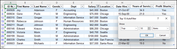
FIGURE 2-2: Using the Top 10 Items AutoFilter to filter out all records except for those with the top ten salaries. (Sample workbook: Employee Table.xlsx)
You can also change the filtering criteria in the Top 10 AutoFilter dialog box before you filter the data. You can choose between Top and Bottom in the leftmost drop-down list box and between Items and Percent in the rightmost one. You can also change the number in the middle combo box by clicking it and entering a new value or using the spinner buttons to select one.
Filtering a table on a field’s font and fill colors or cell icons
Just as you can sort a table using the font or fill color or cell icons that you’ve assigned with the Conditional Formatting feature to values in the field that are within or outside of certain parameters (see the section on the Conditional Formatting feature in Book 2, Chapter 2 for details), you can also filter the table.
To filter a table on a font color, fill color, or cell icon used in a field, you click its AutoFilter button and then select the Filter by Color option from the drop-down menu. Excel then displays a submenu from which you choose the font color, fill color, or cell icon to use in the sort:
- To filter the table so that only the records with a particular font color in the selected field — assigned with the Conditional Formatting Highlight Cell Rules or Top/Bottom Rules options — appear in the table, click its color swatch in the Filter by Font Color submenu.
- To filter the table so that only the records with a particular fill color in the selected field — assigned with the Conditional Formatting Highlight Cell Rules, Top/Bottom Rules, Data Bars, or Color Scales options — appear in the table, click its color swatch in the Filter by Font Color submenu.
- To filter the table so that only the records with a particular cell icon in the selected field — assigned with the Conditional Formatting Icon Sets options — appear in the table, click the icon in the Filter by Cell Icon submenu.
Custom AutoFilter at your service
You can click the Custom Filter option on a field’s Text Filters, Date Filters, or Number Filters continuation menu to open the Custom AutoFilter dialog box, where you can specify your own filtering criteria by using conditions with the AND or OR logical operators (called AND OR conditions for short). When you click the Custom Filter option, Excel opens the Custom AutoFilter dialog box, similar to the one shown in Figure 2-3 (sample workbook: Employee Table.xlsx).
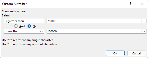
FIGURE 2-3: Using Custom AutoFilter to filter out records except for those within a range of salaries. (Sample workbook: Employee Table.xlsx)
Here, you select the type of operator to use in evaluating the first and second conditions in the top and bottom drop-down list boxes and the values to be evaluated in the first and second conditions in the associated combo boxes. You also specify the type of relationship between the two conditions with the And option button. (The And option button is selected by default.)
When selecting the operator for the first and second condition in the leftmost drop-down list boxes at the top and bottom of the Custom AutoFilter dialog box, you have the following choices, depending on the types of entries in the selected field:
- Equals: Matches records where the entry in the field is identical to the text, date, or number you enter in the associated combo box.
- Does Not Equal: Matches records where the entry in the field is anything other than the text, date, or number you enter in the associated combo box.
- Is After: Matches records where the entry in the date field comes after the date you enter or select in the associated combo box.
- Is After or Equal To: Matches records where the entry in the date field comes after or is the same as the date you enter or select in the associated combo box.
- Is Before: Matches records where the entry in the date field precedes the date you enter or select in the associated combo box.
- Is Before or Equal To: Matches records where the entry in the date field precedes or is the same as the date you enter or select in the associated combo box.
- Is Greater Than: Matches records where the entry in the field follows the text in the alphabet, comes after the date, or is larger than the number you enter in the associated combo box.
- Is Greater Than or Equal To: Matches records where the entry in the field follows the text in the alphabet or is identical, the date comes after or is identical, or the number is larger than or equal to the one you enter in the associated combo box.
- Is Less Than: Matches records where the entry in the field comes before the text in the alphabet, comes before the date, or is less than the number you enter in the associated combo box.
- Is Less Than or Equal To: Matches records where the entry in the field comes before the text in the alphabet or is identical, the date comes before or is identical, or the number is less than or equal to the one you enter in the associated combo box.
- Begins With: Matches records where the entry in the field starts with the text, the part of the date, or the number you enter in the associated combo box.
- Does Not Begin With: Matches records where the entry in the field starts with anything other than the text, the part of the date, or the number you enter in the associated combo box.
- Ends With: Matches records where the entry in the field ends with the text, the part of the date, or the number you enter in the associated combo box.
- Does Not End With: Matches records where the entry in the field ends with anything other than the text, the part of the date, or the number you enter in the associated combo box.
- Contains: Matches records where the entry in the field contains the text, the part of the date, or the number you enter in the associated combo box.
- Does Not Contain: Matches records where the entry in the field contains anything other than the text, the part of the date, or the number you enter in the associated combo box.
 Note that you can use the Begins With, Ends With, and Contains operators and their negative counterparts when filtering a text field — you can also use the question mark (?) and asterisk (*) wildcard characters when entering the values for use with these operators. (The question mark wildcard stands for individual characters, and the asterisk stands for one or more characters.) You use the other logical operators when dealing with numeric and date fields.
When specifying the values in the associated combo boxes on the right side of the Custom AutoFilter dialog box, you can type the text, number, or date, or you can select an existing field entry by clicking the box’s drop-down list button and then clicking the entry on the drop-down menu. In date fields, you can select the dates directly from the date drop-down palette opened by clicking the box’s Date Picker button (the one with the calendar icon).
Figure 2-3 illustrates setting up filtering criteria in the Custom AutoFilter dialog box that selects records whose Salary values fall within two separate ranges of values. In this example, I’m using an OR condition to filter out all records where the salaries fall below $100,000 or are greater than $75,000 by entering the following complex condition:
Salary Is Greater Than 75000 OR Is Less Than 100000
Using the Advanced Filter
When you use advanced filtering, you don’t use the field’s AutoFilter buttons and associated drop-down menu options. Instead, you create a so-called criteria range somewhere on the worksheet that contains the table to be filtered before opening the Advanced Filter dialog box.
When you use the Advanced Filter feature to do a query, you extract copies of the records that match your criteria by creating a subset of the table. You can locate the criteria range to the right of the table and then specify the Copy To range underneath the criteria range, similar to the arrangement shown in Figure 2-4 (sample workbook: Employee Table with Criteria Range.xlsx).
To create a criteria range, you copy the names of the fields in the table to a new part of the worksheet and then enter the values (text, numbers, or formulas) that are to be used as the criteria in filtering the table in rows underneath. When setting up the criteria for filtering the table, you can create either comparison criteria or calculated criteria.
After you’ve set up your criteria range with all the field names and the criteria that you want used, you click the Data tab's Advanced command (or press Alt+AQ) to open the Advanced Filter dialog box similar to the one shown in Figure 2-4. Here, you specify whether you just want to filter the records in the table (by hiding the rows of all those that don’t meet your criteria) or you want to copy the records that meet your criteria to a new area in the worksheet (by creating a subset of the table).

FIGURE 2-4: Using Advanced Filter to copy records that meet the criteria in the Criteria Range. (Sample workbook: Employee Table with Criteria Range.xlsx)
To just filter the data in the table, leave the Filter the List, In-Place option button selected. To query the table and copy the data to a new place in the same worksheet (note that the Advanced Filter feature doesn’t let you copy the data to another sheet or workbook), you select the Copy to Another Location option button. When you select this option button, the Copy To text box becomes available, along with the List Range and Criteria Range text boxes.
To specify the table that contains the data that you want to filter or query, click the List Range text box and then enter the address of the cell range or select it directly in the worksheet by dragging through its cells. To specify the range that contains a copy of the field names along with the criteria entered under the appropriate fields, you click the Criteria Range text box and then enter the range address of this cell range or select it directly in the worksheet by dragging through its cells. When selecting this range, be sure that you include all the rows that contain the values that you want evaluated in the filter or query.
If you’re querying the table by copying the records that meet your criteria to a new part of the worksheet (indicated by clicking the Copy to Another Location option button), you also click the Copy To text box and then enter the address of the cell that is to form the upper-left corner of the copied and filtered records or click this cell directly in the worksheet.
After specifying whether to filter or query the data and designating the ranges to be used in this operation, click OK to have Excel apply the criteria that you’ve specified in the criteria range in either filtering or copying the records.
After filtering a table, you may feel that you haven’t received the expected results — for example, no records are listed under the field names that you thought should have several. You can bring back all the records in the table by clicking the Data tab's Clear command or by pressing Alt+AC. Now you can fiddle with the criteria in the criteria range text box and try the whole advanced filtering thing all over again.
Specifying comparison criteria
Entering selection criteria in the Criteria Range for advanced filtering is very similar to entering criteria in the data form after selecting the Criteria button. However, you need to be aware of some differences. For example, if you are searching for the last name Paul and enter the label Paul in the criteria range under the cell containing the field name Last Name, Excel matches any last name that begins with P-a-u-l such as Pauley, Paulson, and so on. To avoid having Excel match any other last name beside Paul, you would have to enter a formula in the cell below the one with the Last Name field name, as in
="Paul"
When entering criteria for advanced filtering, you can also use the question mark (?) or the asterisk (*) wildcard character in your selection criteria just like you do when using the data form to find records. If, for example, you enter J*n under the cell with the First Name field name, Excel considers any characters between J and n in the First Name field to be a match including Joan, Jon, or John as well as Jane or Joanna. To restrict the matches to just those names with characters between J and n and to prevent matches with names that have trailing characters, you need to enter the following formula in the cell:
="J*n"
When you use a selection formula like this, Excel matches names such as Joan, Jon, and John but not names such as Jane or Joanna that have a character after the n.
When setting up selection criteria, you can also use the other comparative operators, including >, >=, <, <=, and <>, in the selection criteria. See Table 2-1 for descriptions and examples of usage in selection criteria for each of these logical operators.
TABLE 2-1 The Comparative Operators in the Selection Criteria
Operator | Meaning | Example | Locates |
|---|---|---|---|
= | Equal to | =“CA” | Records where the state is CA |
> | Greater than | >m | Records where the name starts with a letter after M (that is, N through Z) |
>= | Greater than | >=3/4/02 | Records where the date is on or after or equal to March 4, 2002 |
< | Less than | <d | Records where the name begins with a letter before D (that is, A, B, or C) |
<= | Less than | <=12/12/04 | Records where the date is on or before or equal to December 12, 2004 |
<> | Not equal to | <>“CA” | Records where the state is not equal to CA |
To find all the records where a particular field is blank in the database, enter = and press the spacebar to enter a space in the cell beneath the appropriate field name. To find all the records where a particular field is not blank in the database, enter <> and press the spacebar to enter a space in the cell beneath the appropriate field name.
Setting up logical AND logical OR conditions
When you enter two or more criteria in the same row beneath different field names in the Criteria Range, Excel treats the criteria as a logical AND condition and selects only those records that meet both criteria. Figure 2-5 (sample workbook: Employee Table with Criteria Range.xlsx) shows an example of the results of a query that uses an AND condition. Here, Excel has copied only those records where the location is Boston and the date hired is before January 1, 2000, because both the criteria Boston and <1/1/00 are placed in the same row (row 2) under their respective field names, Location and Date Hired.
When you enter two or more criteria in different rows of the Criteria Range, Excel treats the criteria as a logical OR and selects records that meet any one of the criteria they contain. Figure 2-6 (sample workbook: Employee Table with Criteria Range.xlsx) shows you an example of the results of a query using an OR condition. In this example, Excel has copied records where the location is either Boston or San Francisco because Boston is entered under the Location field name in the second row (row 2) of the Criteria Range above San Francisco entered in the third row (row 3).

FIGURE 2-5: Copied records where the location is Boston and the date hired is prior to January 1, 2000. (Sample workbook: Employee Table with Criteria Range.xlsx)

FIGURE 2-6: Copied records where the location is Boston and the date hired prior to January 1, 2000 or the location is San Francisco location for any date hired. (Sample workbook: Employee Table with Criteria Range.xlsx)
When creating OR conditions, you need to remember to redefine the Criteria Range to include all the rows that contain criteria, which in this case is the cell range L2:U3. (If you forget, Excel uses only the criteria in the rows included in the Criteria range.)
When setting up your criteria, you can combine logical AND and logical OR conditions (again, assuming you expand the Criteria Range sufficiently to include all the rows containing criteria). For example, if you enter Boston in cell R2 (under Location) and <1/1/00 in cell S2 (under Date Hired) in row 2 and enter San Francisco in cell R3 and then repeat the query, Excel copies the records where the location is Boston and the date hired is before January 1, 2000, as well as the records where the location is San Francisco (regardless of the date hired).
Setting up calculated criteria
You can use calculated criteria when filtering or querying your table. All you need to do is enter a logical formula that Excel can evaluate as either TRUE or FALSE in the Criteria Range under a made-up name that is not any field name used in the table (I repeat, is not a field name in the table). Calculated criteria enable you to filter or query records based on a comparison of entries in a particular field with entries in other fields of the table or based on a comparison with entries in the worksheet that lie outside the table itself.
Figure 2-7 (sample workbook: Employee Table with Calculated Criteria.xlsx) shows an example of using a calculated criterion that compares values in a field to a calculated value that isn’t actually entered in the table. Here, you want to perform a query that copies all the records from the Employee table where the employee’s salary is above the average salary. In this figure, cell V2 contains the formula that uses the AVERAGE function to compute average employee salary and then compares the first salary entry in cell F2 of the table to that average with the following formula:
=F2 > AVERAGE($F$2:$F$33)
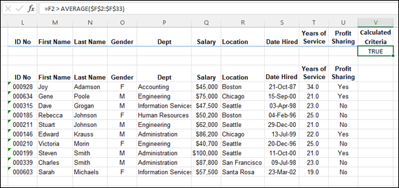
FIGURE 2-7: Copied records extracted from the table for employees whose salaries are above the salary average. (Sample workbook: Employee Table with Calculated Crtieria.xlsx)
Note that this logical formula is placed under the label Calculated Criteria in cell V2, which has been added to the end of the criteria range. Cell F2 is the first cell in the table that contains a salary entry. The cell range, $F$2:$F$33, used as the argument of the AVERAGE function, is the range in the Salary field that contains all the salary entries.
To use this calculated criterion, you must remember to place the logical formula under a name that isn’t used as a field name in the table itself. (In this example, the label Calculated Criteria does not appear anywhere in the row of field names.) You must include this label and formula in the Criteria Range. (For this query example, the criteria range is defined as the range L2:V2.)
When you then perform the query by using the Advanced Filter feature, Excel applies this calculated criterion to every record in the database. Excel does this by adjusting the first Salary field cell reference F2 (entered as a relative reference) as the program examines the rest of the records below. Note, however, that the range reference specified as the argument of the AVERAGE function is entered as an absolute reference ($F$2:$F$33) in the criterion formula so that Excel won’t adjust this reference but compare the Salary entry for each record to AVERAGE computed for this entire range (which just happens to be 40,161).
When entering formulas for calculated criteria that compare values outside the table to values in a particular field, you should always reference the cell containing the very first entry for that field to ensure that Excel applies your criteria to every record in the table.
You can also set up calculated criteria that compare entries in one or more fields to other entries in the table. For example, to extract the records where the Years of Service entry is at least two years greater than the record above it (assuming you have sorted the table in ascending order by years of service), you would enter the following logical formula under the cell labeled Calculated Criteria:
=I3 > I2 + 2
Most often, when referencing cells within the table itself, you want to leave the cell references relative so that they can be adjusted, because each record is examined, and the references to the cells outside the database are absolute so that these won’t be changed when making the comparison with the rest of the records.
When you enter the logical formula for a calculated criterion, Excel returns the logical value TRUE or FALSE. This logical value applies to the field entry for the first record in the table that you refer to in the logical formula. By inspecting this field entry in the database and seeing whether it does indeed meet your intended selection criteria, you can usually tell whether your logical formula is correct.
Using the AND, OR, and NOT functions in calculated criteria
You can also use Excel’s AND, OR, and NOT functions with the logical operators in calculated criteria to find records that fall within a range. For example, to find all the records in the employee database where the salaries range between $55,000 and $75,000, you would enter the following logical formula with the AND function under the cell with the label Calculated Criteria:
=AND(F2 >= 55000, F2 <= 75000)
To find all the records in the Employee table where the salary is either below $29,000 or above $45,000, you would enter the following logical formula with the OR function under the cell with the label Calculated Criteria:
=OR(F2 < 29000, F2 > 45000)
Using the Database Functions
Excel includes several so-called database functions that you can use to calculate statistics, such as the total, average, maximum, minimum, and count in a particular field of the table only when the criteria that you specify are met. For example, you could use the DSUM function in the sample Employee table to compute the sum of all the salaries for employees who were hired after January 1, 2000, or you could use the DCOUNT function to compute the number of records in the table for the Human Resources department.
The database functions, regardless of the difference in names (they all begin with the letter D) and the computations that they perform, all take the same three arguments as illustrated by the DAVERAGE function:
DAVERAGE(database, field, criteria)
The arguments for the database functions require the following information:
- database is the argument that specifies the range containing the table, and it must include the row of field names in the top row.
- field is the argument that specifies the table column from which the values are to be calculated by the database function (averaged in the case of the DAVERAGE function). You can specify this argument by enclosing the name of the field in double quotes (as in “Salary” or “Date Hired”), or you can do this by entering the number of the column in the table (counting from left to right with the first field counted as 1).
- criteria is the argument that specifies the address of the range that contains the criteria that you’re using to determine which values are calculated. This range must include at least one field name that indicates the field whose values are to be evaluated and one cell with the values or expression to be used as the criteria.
Note that in specifying the field argument, you must refer to a column in the table that contains numeric or date data for all the database functions with the exception of DGET. All the rest of the database functions can’t perform computations on text fields. If you mistakenly specify a column with text entries as the field argument for these database functions, Excel returns an error value or 0 as the result. Table 2-2 lists the various database functions available in Excel along with an explanation of what each one calculates. (You already know what arguments each one takes.)
TABLE 2-2 The Database Functions in Excel
Database Function | What It Calculates |
|---|---|
DAVERAGE | Averages all the values in a field of the table that match the criteria you specify. |
DCOUNT | Counts the number of cells with numeric entries in a field of the table that match the criteria you specify. |
DCOUNTA | Counts the number of nonblank cells in a field of the table that match the criteria you specify. |
DGET | Extracts a single value from a record in the table that matches the criteria you specify. If no record matches, the function returns the #VALUE! error value. If multiple records match, the function returns the #NUM! error value. |
DMAX | Returns the highest value in a field of the table that matches the criteria you specify. |
DMIN | Returns the lowest value in a field of the table that matches the criteria you specify. |
DPRODUCT | Multiplies all the values in a field of the table that match the criteria you specify. |
DSTDEV | Estimates the standard deviation based on the sample of values in a field of the table that match the criteria you specify. |
DSTDEVP | Calculates the standard deviation based on the population of values in a field of the table that match the criteria you specify. |
DSUM | Sums all the values in a field of the table that match the criteria you specify. |
DVAR | Estimates the variance based on the sample of values in a field of the table that match the criteria you specify. |
DVARP | Calculates the variance based on the population of values in a field of the table that match the criteria you specify. |
The database functions are too rarely used to rate their own command button on the Ribbon’s Formulas tab. As a result, to use them in a worksheet, you must click the Insert Function (fx) button on the Formula bar, select Database from the Select a Category drop-down list box, and then click the function. You can also type the database function directly into the cell.
Figure 2-8 (sample workbook: Employee Table with Database Function.xlsx) illustrates the use of the database function DSUM. Cell C2 in the worksheet shown in this figure contains the following formula:
=DSUM(Table1[#All], "Salary", F1:F2)

FIGURE 2-8: Using DSUM to total the salaries over $55,000 in the Employee table. (Sample workbook: Employee Table with Database Function.xlsx)
This DSUM function computes the total of all the salaries in the table that are above $55,000. This total is $468,500, as shown in cell C2, which contains the formula.
To perform this calculation, I specified the range A3:J35, which contains the entire table. This range includes the top row of field names as the database argument (which Excel automatically converted to its range name equivalent, Table1[#All]). I then specified “Salary” as the field argument of the DSUM function because this field name contains the values that I want totaled. Finally, I specified the range F1:F2 as the criteria argument of the DSUM function because these two cells contain the criteria range that designate that only the values exceeding 55000 in the Salary field are to be summed.
Querying External Data
Excel enables you to query tables stored in external databases to which you have access and then extract the data that interests you into your worksheet for further manipulation and analysis. These data sources can include Microsoft Access database files, web pages, text files, and other data sources, such as database tables on SQL Server or Oracle, XML data files, and data tables from online connections such as Azure Table Storage.
When importing data from such external sources into your Excel worksheets, you may well be dealing with data stored in multiple related tables all stored in the database (what Excel refers to as a data model). The relationship between different tables in the same database is based on a common field (column) that occurs in each related data table, which is officially known as a key field, but in Excel is generally known as a lookup column. When relating tables on a common key field, in at least one table, the records for that field must all be unique with no duplicates, such as a Clients table where each item in the Customer ID field is unique (where it’s known as the primary key). In the other related table, the common field (known as the foreign key) may or may not be unique as in an Orders data table where a particular entry in its Customer ID field can appear multiple times, as it’s quite permissible (even desirable) to have the same client making multiple purchases.
There’s only one other thing to keep in mind when working with related data tables and that is the type of relationship that exists between the two tables. Two types of relationships are supported in a data model:
- One-to-one relationship where the entries in both the primary and foreign key fields are unique such as a relationship between a Clients table and Discount table where the Customer ID field occurs only once in each table (as each client has only one discount percentage assigned).
- One-to-many relationship where duplicate entries in the foreign key field are allowed, as in a relationship between a Clients table and an Orders table where the Customer ID field may occur multiple times (as the client makes multiple purchases).
Most of the time, Excel can figure out the relationship between the data tables you import. However, if Excel should ever get it wrong or your tables contain more than one common field that could possibly serve as the key, you can manually define the proper relationship. In the Data tab's Data Tools group, select the Relationships button (or press Alt+AA) to open the Manage Relationships dialog box. Click New to open the Create Relationship dialog box, where you define the common field in each of the two related data tables. After creating this relationship, you can use any of the fields in either of the two related tables in reports that you prepare or PivotTables that you create. (See Book 7, Chapter 2 for details on creating and using PivotTables.)
To import data from external database files and tables, you select the Data tab's Get Data drop-down button in the Get & Transform Data group (or press Alt+APN). Excel displays a menu with the following choices:
- From File: Enables you to import data from a file saved on a local or network drive in various file formats, including Excel workbook, text or CSV (Comma Delimited Value), XML (Extensible Markup Language), and JSON (JavaScript Object Notation) file formats.
- From Database: Enables you to import data from tables in a specific type of database file, including SQL Server Database, Microsoft Access, Analysis Services, and SQL Analysis Server Database.
- From Azure: Enables you to import data from an Azure SQL database or one of the various storage spaces available on this Microsoft cloud service (visit
https://azure.microsoft.comfor more information). - From Power BI dataset: Enables you to launch Power BI (Business Intelligence), a Microsoft visual data analytics program, and import data into Excel from the Power BI Data Catalog (see
https://powerbi.microsoft.comfor more information). - From Online Services: Enables you to import data saved on an online service to which you already subscribe, such as Microsoft Exchange Online, Dynamics 365, or Salesforce.
- From Other Sources: Enables you to import data from a variety of sources, including From Sheet (a range or table in the existing workbook) or From Web (tables on a web page) or using existing queries from Microsoft Query, OData Feed, ODBC (Open Database Connectivity), OLEDB (Object Linking and Embedded Database), and Blank Query to create a new query with Excel’s Power Query Editor add-in.
- Combine Queries: Enables you to merge two existing data tables in the current workbook or append one data table to another.
- Launch Power Query Editor: Opens Excel’s Query Editor add-in that enables you to create advanced data queries that connect various data sources and perform complex analysis.
- Data Source Settings: Opens the Data Source Settings dialog box where you can manage permissions for the external data sources that Excel can use in data queries.
- Query Options: Opens the Query Options dialog box where you manage the global and current workbook load and privacy settings.
Retrieving data from Access database tables
To make an external data query to a Microsoft Access database table, choose Data⇒ Get Data⇒ From Database⇒ From Microsoft Access Database (or press Alt+APNDC). Excel opens the Import Data dialog box, where you select the name of the Access database (using the .accdb or .mdb file extension) and then click the Import button.
After Excel establishes a connection with the Access database file, the Navigator dialog box opens, similar to the one shown in Figure 2-9 (sample file: Northwind.accdb). The Navigator dialog box is divided into two panes: Selection on the left and Preview on the right. When you click the name of a data table or query in the Selection Pane, Excel displays a portion of the Access data in the Preview pane on the right. To import multiple (related) data tables from the selected Access database, select the Select Multiple Items check box. Excel then displays check boxes before the name of each table in the database. After you select the check boxes for all the tables you want to import, you have a choice of options:
- Load: Imports the Access file data from the item(s) selected in the Navigator directly into the current worksheet starting at the cell cursor's current position.
- Load⇒ Load To: Opens the Import Data dialog box where you can specify how you want to view the imported Access data (as a worksheet table, a PivotTable, a PivotChart, or as a data connection without importing any data) and where to import the Access data (existing or new worksheet) as well as whether to add the Access data to the worksheet’s data model.
- Transform Data: Displays the Access data table(s) in the Excel Power Query Editor where you can further query and transform the data before importing into the current Excel worksheet with its Close & Load or Close & Load To option.
When you select the Load To option to specify how and where to import the Access data, the Import Data dialog box contains the following options:
- Table: Imports the Access data into an Excel table in either the current or new worksheet — see the “Existing Worksheet” and “New Worksheet” bullets that follow. Note that when you import more than one data table, the Existing Worksheet option is no longer available, and the data from each imported data table is imported to a separate new worksheet in the current workbook.
- PivotTable Report: Imports the Access data into a new PivotTable (see Book 7, Chapter 2) that you can construct with the Access data.

FIGURE 2-9: Using the Navigator to select which data tables and queries from the Northwind Access database to import into the current Excel worksheet. (Sample file: Northwind.accdb)
- PivotChart: Imports the Access data into a new PivotTable (see Book 7, Chapter 2) with an embedded PivotChart that you can construct with the Access data.
- Only Create Connection: Creates a connection to the Access database table(s) that you can use later to import its data.
- Existing Worksheet: Imports the Access data into the current worksheet starting at the current cell address listed in the text box below.
- New Worksheet: Imports the Access data into a new sheet that’s added to the end of the sheets already in the workbook.
- Add This Data to the Data Model: Adds the Access data to the data model already defined in the Excel workbook using relatable, key fields.
- Properties: Opens the drop-down menu with the Import Relationships Between Tables check box (selected by default) and Properties item. Deselect the check box to prevent Excel from recognizing the relationship established between the data tables in Access. Click the Properties button to open the Connection Properties dialog box, where you can modify all sorts of connection properties, including when the Access data’s refreshed in the Excel worksheet and how the connection is made.
Figure 2-10 (sample file: Northwind.accdb) shows you a workbook after importing both the Customers and Orders tables from the sample Northwind Access database as new tables on separate worksheets. When I imported the two data tables, Excel automatically added two new worksheets (named Customers and Orders) to the workbook, while at the same time importing the Customers data table to the Customers sheet and the Orders data table to the Orders sheet.
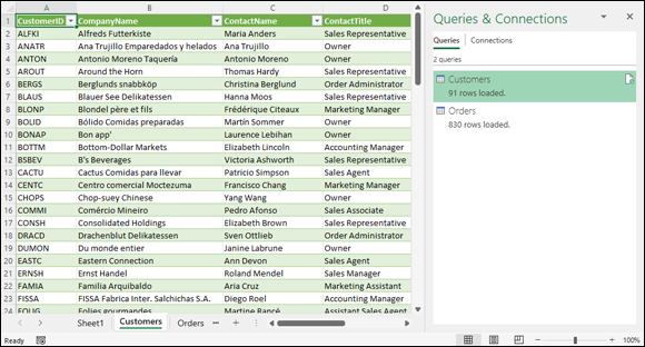
FIGURE 2-10: Customers worksheet with the data imported from the Access Customers data table in the sample Northwind database. (Sample file: Northwind.accdb)
Figure 2-11 (sample file: Northwind.accdb) shows the same new workbook, this time with the Orders worksheet selected and the Manage Relationships dialog box open (by clicking the Data tab's Relationships button or pressing Alt+AA). When Excel imported these two data tables, it automatically picked up on and retained the original relationship between them in the Northwind database, where the CustomerID field is the primary key field in the Customers data table and a foreign key field in the Orders data table.
After importing the external data into one of your Excel worksheets, you can then use the Filter buttons attached to the various fields to sort the data (as described in Book 6, Chapter 1) and filter the data (as described earlier in this chapter).
After you import data from an external source, such as a Microsoft Access database, Excel automatically displays a Queries & Connections task pane with two tabs: Queries, which displays the source(s) of the data imported into the current workbook, and Connections, which displays their connection to the workbook data model (and to each other if there are multiple sources and they are related to each other). If this task pane is not currently displayed in the current worksheet, choose Data⇒ Queries & Connections (or press Alt+AO) to redisplay it.

FIGURE 2-11: Orders worksheet with the data imported from the Orders data table in the sample Northwind database showing the relationship with the Customers table. (Sample file: Northwind.accdb)
Excel keeps a list of all the external data sources and data queries you make to the current workbook so that you can reuse them to import updated data from another database or web page. To quickly reconnect with a data source, click the Data tab's Recent Sources button (or press Alt+PR) to open the Recent Sources dialog box where you click the name of the external file before you select the Connect button. To reuse a query, click the Data tab's Existing Connections button (or press Alt+AX) to open the Existing Connections dialog box to access this list and then click the name of the query to repeat before you click the Open button.
Retrieving data from the web
To make a web page query, choose Data⇒ Get Data⇒ From Other Sources⇒ From Web (or press Alt+AFW). Excel then opens the From Web dialog box containing a URL text box where you specify the address of the web page containing the data you want to import into Excel as in
After you click OK in the From Web dialog box, Excel establishes a connection with the web page before opening the Navigator dialog box (similar to the one shown earlier in Figure 2-9). When you select a table in the list in the Selection pane on the left, Excel displays a preview of the data in the Table View tab of the Preview pane on the right (to display the data more or less as it appears on the web page itself, you click the Web View tab in this pane). To import more than one table of data from a web page, click the Select Multiple Items check box and then click the check boxes in front of the name (Table 1, Table 2, and so on) you want imported.
After you finish checking the table or tables you want to import on the page, you can select one of the following three import options:
- Load: Imports the web data in the tables selected in the Navigator directly into the current worksheet starting at the cell cursor’s current position.
- Load⇒ Load To: Opens the Import Data dialog box where you can choose how you want to view the imported web data (as a worksheet table, PivotTable, PivotChart, or just data connection without importing any data) and where to import the web data (into an existing or new worksheet) as well as whether to add the web data to the worksheet’s data model.
- Transform Data: Display the web data table(s) in the Excel Power Query Editor where you can further query and transform the data before importing into the current Excel worksheet with its Close & Load or Close & Load To option.
After importing your web data into a new or existing worksheet, you can then manipulate the data as you would any other worksheet table, including filtering it and sorting with the AutoFilter buttons.
When working with tables of stock quotes imported from financial websites, such as NASDAQ and MSN Money, during periods when the markets are still open and active, you can use the Data tab's Refresh All command (or press Alt+ARA) to keep the stock prices and trading volume entries in your worksheet up to date.
 You can only make web queries when your computer has Internet access. So, if you’re using Excel on a device that can’t connect to the web at the moment, you won’t be able to perform a new web query until you get to a place where you can get online.
Retrieving data from text files
If you have a text file containing data you need to bring into your worksheet, you can import it by choosing Data⇒ Get Data⇒ From File⇒ From Text/CSV (or press Alt+AFT) and then selecting the file to use in the Import Data dialog box. After you select the text file containing the data you need to retrieve in this dialog box and click its Import button, Excel opens the Navigator dialog box with the name of the text or CSV (Comma Separated Value) file as its title.
This version of the Navigator, as shown in Figure 2-12 (sample file: Employees.txt), automatically scans and analyzes the data in the text or CSV file and attempts to correctly split up (or parse) its data into separate cells of the worksheet based on what Excel character the program determines is the standard character used to separate each data item (such as a comma or tab) in every line, just as it uses the character for the Enter key to mark the separation of each line of data within the file.

FIGURE 2-12: Importing the data in a tab-delimited text file into a worksheet using the options in Navigator dialog box. (Sample file: Employees.txt)
Text files that use the comma to separate data items are known as CSV files (for Comma Separated Values). Those that use tabs to separate the individual data items are known as tab delimited files. Note that some programs use the generic term, delimited files, to refer to any text file that uses a standard character, such as a comma or tab, to separate its individual data items.
If Excel has correctly parsed the data in your text or CSV file as shown in the preview in the Navigator, you can then select one of the following three import options to bring the data into your worksheet:
- Load: Imports the parsed text data previewed in the Navigator directly into the current worksheet starting at the cell cursor’s current position.
- Load⇒ Load To: Opens the Import Data dialog box where you can choose how you want to view the imported text data (as a worksheet table, PivotTable, PivotChart, or just data connection without importing any data) and where to import the text data (into an existing or new worksheet) as well as whether to add the text data to the worksheet’s data model.
- Transform Data: Displays the parsed text data in the Excel Power Query Editor where you can further query and transform the data before importing into the current Excel worksheet with its Close & Load or Close & Load To option.
If Excel has not correctly parsed the data in your text or CSV file in the preview in the Navigator, you can try changing one of the three settings used in determining how the data is parsed before proceeding with any kind of import:
- File Origin: Select a new text file type based on its country code on the File Origin drop-down menu.
- Delimiter: Select a new delimiting character on the Delimiter drop-down menu to be used in parsing the data into separate cells.
- Data Type Detection: Change the number of rows used in trying to determine whether the parsed data is a number, date, or text value either by selecting the Based on Entire Dataset option on the Data Type Detection drop-down menu to use all the rows in the file or select Do Not Detect Data Types option to prevent Excel from trying to differentiate the data types.
If Excel still can’t correctly parse your text or CSV file in the preview and insists on importing each row of text data into a single column, all is not lost. You can still go ahead with the import and then after bringing the data of the text file into a new or existing worksheet, use the Convert to Text Wizard to correctly parse it into separate columns.
To do this, select the cells with the imported text data. then click the Data tab's Text to Columns command (or press Alt+AE). Excel opens the Convert Text to Columns Wizard - Step 1 of 3 dialog box. Here, you choose between the Delimited and Fixed Width option determine how the data is to be separated before clicking the Next button to open the Convert Text to Columns Wizard - Step 2 of 3 dialog box.
In the Step 2 of 3 dialog box when you previously selected the Delimited option in the Step 1 of 3 dialog box, you need to select the delimiting character if the wizard selects the wrong character in the Delimiters section before clicking the Next button. If your text file uses a custom delimiting character, you need to select the Other check box and then enter that character in its text box. If your file uses two consecutive characters (such as a comma and a space), you need to select their check boxes as well as the Treat Consecutive Delimiters As One check box.
By default, the Convert Text to Columns Wizard treats any characters enclosed in a pair of double quotes as text entries (as opposed to numbers). If your text file uses a single quote, click the single quote (‘) character in the Text Qualifier drop-down list box.
If, instead, you selected the Fixed Width option in the Step 1 of 3 dialog box, the Step 2 of 3 dialog box previews the column breaks that indicate how the text data appears when split apart into separate columns of the worksheet. You can then modify the column breaks in the preview with your mouse. Click in the sample data shown in the Data Preview area to create new column breaks and modify the extent of the breaks by dragging their borders. When the column breaks in the data preview appear correct, click the Next button to open the Convert Text to Columns Wizard - Step 3 of 3 dialog box.
In the Step 3 of 3 dialog box, you get to assign a data type to the various columns of text data or indicate that a particular column of data should be skipped and therefore not imported into your Excel worksheet.
When setting data formats for the columns of the text file, you can choose among the following three data types:
- General (the default) to convert all numeric values to numbers, entries recognized as date values to dates, and everything else in the column to text
- Text to convert all the entries in the column to text
- Date to convert all the entries to dates by using the date format shown in the associated drop-down list box
To assign one of the three data types to a column, click its column in the Data Preview section and then click the appropriate radio button (General, Text, or Date) in the Column Data Format section in the upper-left corner.
In determining values when using the General data format, Excel uses the period (.) as the decimal separator and the comma (,) as the thousands separator. If you’re dealing with data that uses these two symbols in just the opposite way (the comma for the decimal and the period for the thousands separator), as is the case in many European countries, click the Advanced button in the Step 3 of 3 dialog box to open the Advanced Text Import Settings dialog box. There, select the comma (,) in the Decimal Separator drop-down list box and the period (.) in the Thousands Separator drop-down list box before you click OK. If your text file uses trailing minus signs (as in 100–) to represent negative numbers (as in −100), make sure that the Trailing Minus for Negative Numbers check box contains a check mark.
If you want to change the date format for a column to which you’ve assigned the Date data format, click its M-D-Y code in the Date drop-down list box (where M stands for the month, D for the day, and Y for the year).
To skip the importing of a particular column, click it in the Data Preview and then select the Do Not Import Column (Skip) option button at the bottom of the Column Data Format section.
After you have all the columns formatted as you want, click the Finish button in the Convert Text to Columns – Step 3 of 3 dialog box. Excel then splits the entries in the imported text file into separate columns of the current worksheet, and all that’s left for you to do is, perhaps, adjust the column widths to suit.
Querying data from other data sources
Database tables created and maintained with Microsoft Access are not, of course, the only external database sources on which you can perform external data queries. To import data from other sources, choose Data⇒ Get Data⇒ From Database (or press Alt+APND) to open a drop-down menu with other database options including:
- From SQL Server Database to import data from an SQL server database.
- From Analysis Services to import data from an SQL Server Analysis cube.
- From SQL Server Analysis Services Database (Import) to import data from an SQL server database using an optional MDX or DAX query.
In addition, the From Other Sources option on the Get Data drop-down menu offers you the following querying choices:
- From Sheet to create a new query in the Power Query Editor using the selected Excel data table or named cell range in the current worksheet (same as clicking the From Table/Range command button on the Ribbon’s Data tab).
- From Web to import data from a web page (same as clicking the From Web command button on the Ribbon’s Data tab).
- From Microsoft Query to import data from a database table using Microsoft Query that follows the ODBC (Open DataBase Connectivity) standards.
- From SharePoint List to import data from a Microsoft SharePoint website.
- From OData Feed to import data from any database table following the Open Data Protocol (shortened to OData) — note that you must provide the file location (usually a URL) and user ID and password to access the OData data feed before you can import any of its data into Excel.
- From Hadoop File (HDFS) to import data from a Hadoop Distributed File System.
- From Active Directory to import data from the Microsoft Active Directory service for Windows domain networks.
- From Microsoft Exchange to import data from a Microsoft Exchange Server.
- From ODBC to import data from a database that follows Microsoft’s ODBC (Open Database Connectivity) standards.
- From OLEDB to import data from a database that follows the OLEDB (Object Linked Embedded Database) standards.
- Blank Query to create a brand-new database query in the Power Query Editor.
Transforming a data query in the Power Query Editor
Whenever you do a data query in Excel using the From Text/CSV, From Web, or From Sheet command buttons on the Ribbon’s Data tab, you have the option of transforming that query in the Power Query Editor. When you do an external query with the From Text/CSV, or From Web options, you open the Power Query Editor after specifying the data table(s) to import into Excel by clicking Transform Data button in the Navigator dialog box. However, whenever you use the From Sheet command to designate a selected cell range in the current worksheet as a data table, Excel automatically opens the data table in a new Power Query Editor window so that you can create or transform an existing query.
Although the subject of using the Power Query Editor to perform advanced queries is well beyond the scope of this book, basic use of the Power Query Editor should prove to be no problem as the Power Query Editor’s interface and essential features are very similar to those of Excel.
Figure 2-13 (sample workbook: Contoso Stores.xlsx) shows the Power Query Editor window after opening it to create a new query with the Contoso Stores table. To create the new query, I select a cell in the table before choosing Data⇒ Get Data⇒ From Sheet.
As you see in this figure, in the Power Query Editor, the imported Excel client data table retains its worksheet row and column arrangement with the column headings complete with Auto-Filter drop-down buttons intact. Above the data table, the Power Query Editor sports a Ribbon type command structure with a File menu followed by four tabs: Home, Transform, Add Column, and View. To the right of the imported data table, a Query Settings task pane appears that not only displays the source of the data (a table named Table1) but also all the steps applied in building this new query.

FIGURE 2-13: Creating a new query in the Power Query Editor using a data table created in an Excel worksheet. (Sample workbook: Contoso Stores.xlsx)
Once the Contoso Store data records are loaded into the Power Query Editor, I can use its commands to query the data before returning the subset of records to a new worksheet in Excel. For this query, I am interested in creating a subset of records where the status of the store is On and the number of employees is greater than 100. To do this, I use the AutoFilter buttons on the Status and EmployeeCount fields, as shown in Figure 2-14 (sample workbook: Contoso Stores.xlsx) to filter the records to display just those with On in the Status field and with the Greater Than number filter set to 100 for the EmployeeCount field. Then, I sort the records from the highest to lowest employee count by sorting on the EmployeeCount field in descending order. After that, I’m ready to select the Close & Load To option on the Close & Load command button on the Home tab to save my query and load it into a new worksheet in the current workbook. To do this, I accept the default settings of Table and New Worksheet in the Import Data dialog box that appears after selecting the Close & Load To option prior to clicking OK.
Figure 2-15 shows the results. Here you see the new Excel worksheet that the Editor created before it copied the filtered and sorted the subset of the Contoso Stores records into a new data table in cell range A1:Y4. When the Power Query Editor imported this new data table, the program also assigned it a table style, added AutoFilter buttons, and opened a Queries & Connections task pane. Now all that’s left to do is a bit of formatting and renaming the worksheet.

FIGURE 2-14: Setting the filtering and sorting criteria for the new data query in the Power Query Editor. (Sample workbook: Contoso Stores.xlsx)

FIGURE 2-15: The Contoso Stores data queried in the Power Query Editor after loading it into a new Excel worksheet.