
Chapter 17
THE INTERNAL RATE OF RETURN
A well-deserved return
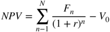
If net present value (NPV) is inversely proportional to the discounting rate, then there must exist a discounting rate that makes NPV equal to zero.
To apply this concept to capital expenditure, simply replace “yield to maturity” by “IRR”, as the two terms mean the same thing. It is just that one is applied to financial securities (yield to maturity) and the other to capital expenditure (IRR).
Section 17.1 CALCULATING YIELD TO MATURITY
To calculate yield to maturity, make r the unknown and simply use the NPV formula again. The rate r is determined as follows:
To use the same example from Section 16.4:
In other words, an investment's yield to maturity is the rate at which its market value is equal to the present value of the investment's future cash flows.
In our illustration, the IRR is about 28.6% (see figure in Section 16.4).
Section 17.2 YIELD TO MATURITY AS AN INVESTMENT CRITERION
The yield to maturity is frequently used in financial markets because it represents for the investor the return to be expected for a given level of risk, which they can then compare to their required return rate, thereby simplifying the investment decision.
The decision-making rule is very simple: if an investment's yield to maturity is higher than the investor's required return, they will make the investment or buy the security. Otherwise, they will abandon the investment or sell the security.
In our example, since the yield to maturity (28.6%) is higher than the return demanded by the investor (20%), they should make the investment. If the market value of the same investment were 3 (and not 2), the yield to maturity would be 10.4%, and they should not invest.
Hence, at fair value, the yield to maturity is identical to the market's required return. In other words, net present value is nil (this will be developed further in Chapter 26).
Section 17.3 THE LIMITS OF YIELD TO MATURITY OR IRR
With this new investment-decision-making criterion, it is now necessary to consider how IRR can be used vis-à-vis net present value. It is also important to investigate whether or not these two criteria could somehow produce contradictory conclusions.
If it is a simple matter of whether or not to buy into a given investment, or whether or not to invest in a project, then the two criteria produce exactly the same result, as shown in the example.
If the cash flow schedule is the same, then calculating the NPV by choosing the discounting rate and calculating the internal rate of return (and comparing it with the discounting rate) are two sides of the same mathematical coin.
The issue is, however, a bit more complex when it comes to choosing between several securities or projects, which is usually the case. Comparing several streams of cash flows (securities) should make it possible to choose between them.
1/ THE REINVESTMENT RATE AND THE MODIFIED IRR (MIRR)
Consider two investments A and B, with the following cash flows:
| Year | 1 | 2 | 3 | 4 | 5 | 6 | 7 |
|---|---|---|---|---|---|---|---|
| Investment A | 6 | 0.5 | |||||
| Investment B | 2 | 3 | 0 | 0 | 2.1 | 0 | 5.1 |
At a 5% discount rate, the present value of investment A is 6.17 and that of investment B is 9.90. If investment A's market value is 5, its net present value is 1.17. If investment B's market value is 7.5, its net present value is 2.40.
Now calculate the IRR. It is 27.8% for investment A and 12.7% for investment B. Or, to sum up:
| NPV at 5% | IRR% | |
|---|---|---|
| Investment A | 1.17 | 27.8 |
| Investment B | 2.40 | 12.7 |
Investment A delivers a rate of return that is much higher than the required return (27.8% vs. 5%) during a short period of time. Investment B's rate of return is much lower (12.7% vs. 27.8%), but is still higher than the 5% required return demanded and is delivered over a far longer period (seven years vs. two). Our NPV and internal rate of return models are telling us two different things. So, should we buy investment A or investment B?
At first glance, investment B would appear to be the more attractive of the two. Its NPV is higher and it creates the most value: 2.40 vs. 1.17.
However, some might say that investment A is more attractive, as cash flows are received earlier than with investment B and therefore can be reinvested sooner in high-return projects. While that is theoretically possible, it is the strong (and optimistic) form of the theory because competition among investors and the mechanisms of arbitrage tend to move net present values towards zero. Net present values moving towards zero means that exceptional rates of return converge towards the required rate of return, thereby eliminating the possibility of long-lasting high-return projects.
Given the convergence of the exceptional rates towards required rates of return, it is more reasonable to suppose that cash flows from investment A will be reinvested at the required rate of return of 5%. The exceptional rate of 27.8% is unlikely to be recurrent.
And this is exactly what happens if we adopt the NPV decision rule. The NPV in fact assumes that the reinvestment of interim cash flows is made at the required rate of return. The IRR assumes that the reinvestment rate of interim cash flows is simply the IRR itself. However, in equilibrium, it is unreasonable to think that the company can continue to invest at the same rate of the (sometimes) exceptional IRR of a specific project. Instead, it is much more reasonable to assume that, at best, the company can invest at the required rate of return.
However, a solution to the reinvestment rate problem of IRR is the modified IRR (MIRR).
So, by capitalising cash flow from investments A and B at the required rate of return (5%) up to period 7, we obtain from investment A in period 7: 6 × 1.0056 + 0.5 × 1.055, or 8.68. From investment B we obtain 2 × 1.056 + 3 × 1.055 + 2.1 × 1.052 + 5.1, or 13.9. The internal rate of return that allows for investment A in capitalising over seven years to reach 8.68 is 8.20%; it is often called modified IRR. For investment B, the modified IRR is 9.24%.
We have thus reconciled the NPV and internal rate of return models.
Some might say that it is not consistent to expect investment A to create more value than investment B, as only 5 has been invested in A vs. 7.5 for B. Even if we could buy an additional “half-share” of A, in order to equalise the purchase price, the NPV of our new investment in A would only be 1.17 × 1.5 = 1.76, which would still be less than investment B's NPV of 2.40. For the reasons discussed above, we are unlikely to find another investment with a return identical to that of investment A.
Instead, we should assume that the 2.5 in additional investment would produce the required rate of return (5%) for seven years. In this case, NPV would remain, by definition, at 1.17, whereas the internal rate of return of this investment would fall to 11%. NPV and the internal rate of return would once again lead us to conclude that investment B is the more attractive investment.
In fact, the NPV criterion is a better choice criterion than the IRR because it assumes that the intermediate flows of the investment are reinvested at the required rate of return (the discount rate), whereas in the calculation of the IRR they are assumed to be reinvested at that rate. The latter assumption is very strong because, if the IRR is higher than the required rate of return, it assumes that the company will always find projects that yield more than the required rate of return.
2/ MULTIPLE OR NO IRR
Finally, there are some rare cases where the use of the IRR leads to a deadlock. Consider the following investments:
| Year | 0 | 1 | 2 |
|---|---|---|---|
| Project A | 4 | −7 | 4 |
| Project B | −1 | 7.2 | −7.2 |
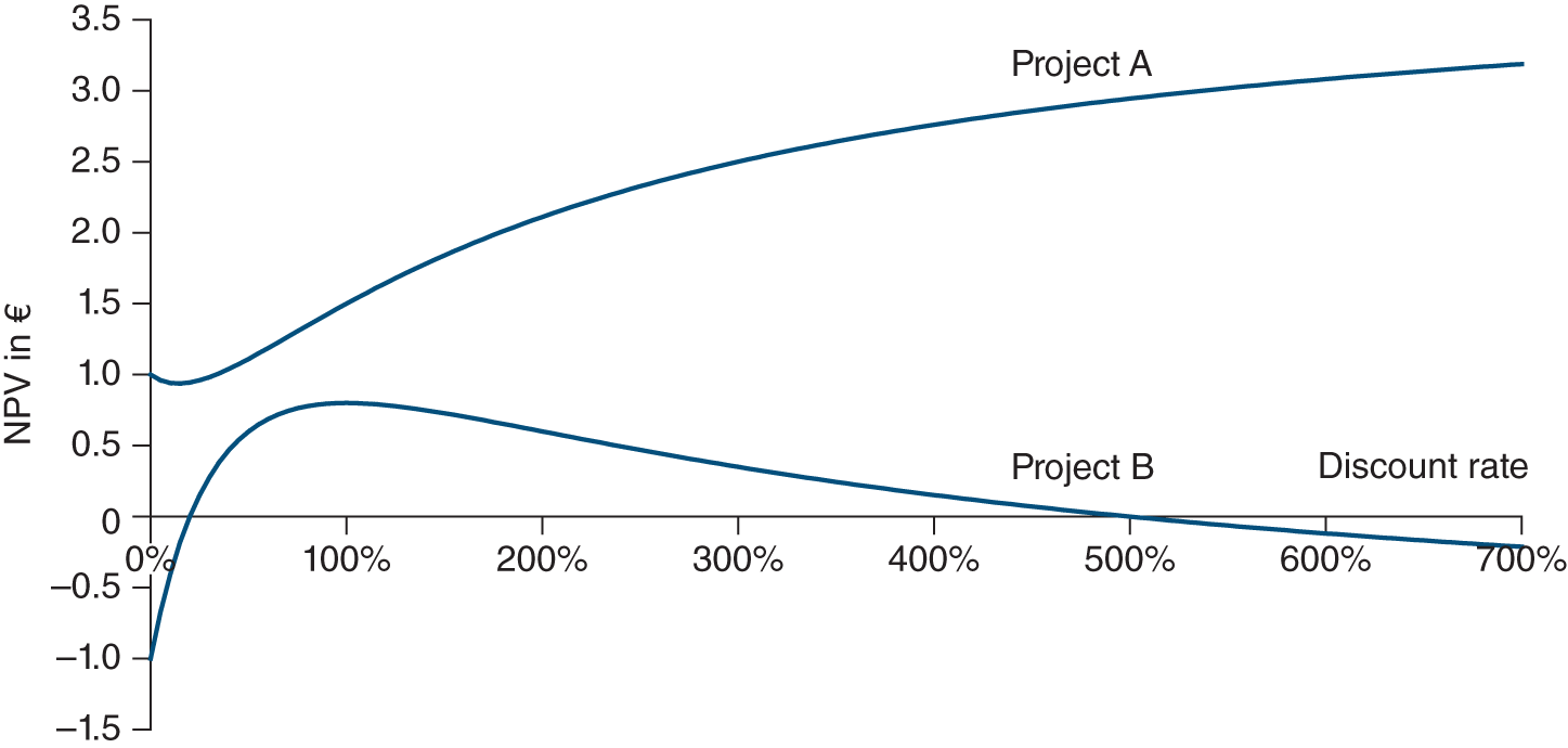
Project A has no IRR. Thus, we have no benchmark for deciding if it is a good investment or not. Although the NPV remains positive for all the discount rates, it remains only slightly positive and the company may decide not to do it.
Project B has two IRRs, and we do not know which is the right one. There is no good reason to use one over the other. Investments with “unconventional” cash flow sequences are rare, but they can happen. Consider a firm that is cutting timber in a forest. The timber is cut, sold and the firm gets an immediate profit. But, when harvesting is complete, the firm may be forced to replant the forest at considerable expense.
The IRR criterion does not allow for the ranking of different investment opportunities. It only allows us to determine whether one project yields at least the return required by investors. When the IRR does not allow us to judge whether an investment project should be undertaken or not (e.g. no IRR or several IRRs), the NPV should be analysed.
Section 17.4 EFFECTIVE ANNUAL RATE, NOMINAL RATES AND PROPORTIONAL RATES
We have just discovered the IRR, but many readers will be more aware of the interest rate, especially those planning to take out a loan. How can we reconcile the two?
Consider someone who wants to lend you €1,000 today at 10% for four years. This 10% means 10% per year and constitutes the nominal rate of return of your loan. This rate will be the basis for calculating interest, proportional to the time elapsed and the amount borrowed. Assume that you will pay interest annually, at the end of each annual period rather than at the beginning.
1/ THE CONCEPT OF EFFECTIVE ANNUAL RATE
Now what happens when interest is paid not once but several times per year?
Suppose that somebody lends you money at 10% but says (somewhere in the fine print at the bottom of the page) that interest will have to be paid on a half-yearly basis. For example, suppose you borrowed €100 on 1 January and then had to pay €5 in interest on 1 July and €5 on 1 January of the following year, as well as the €100 in principal at the same date.
This is not the same as borrowing €100 and repaying €110 one year later. The amount of interest may be the same (5 + 5 = 10), but the payment schedule is not. In the first case, you will have to pay €5 on 1 July (just before leaving on summer holiday), which you could have kept until the following 1 January in the second case. In the first case you pay €5, instead of investing it for six months as you could have done in the second case.
As a result, the loan in the first case costs more than a loan at 10% with interest due annually. Its effective rate is not 10%, since interest is not being paid on the benchmark annual terms.
To avoid comparing apples and oranges, a financial officer must take into account the effective date of disbursement. We know that one euro today is not the same as one euro tomorrow. Obviously, the financial officer wants to postpone expenditure and accelerate receipts, thereby having the money work for them. So, naturally, the repayment schedule matters when calculating the rate.
Which is the best approach to take? If the interest rate is 10%, with interest payable every six months, then the interest rate is 5% for six months. We then have to calculate an effective annual rate (and not for six months), which is our point of reference and our constant concern.
Two rates referring to two different maturities are said to be equivalent if the future value of the same amount at the same date is the same with the two rates.
In our example, the lender receives €5 on 1 July which, compounded over six months, becomes 5 + (10% × 5) / 2 = €5.25 on the following 1 January, the date on which they receive the second €5 interest payment. So, over one year, they will have received €10.25 in interest on a €100 investment.
Therefore, the effective annual rate is 10.25%. This is the real cost of the loan, since the return for the lender is equal to the cost for the borrower.
If the apparent rate (or nominal rate) (ra) is to be paid n times per year, then the effective annual rate (t) is obtained by compounding this nominal rate n times after first dividing it by n:
where n is the number of interest payments in the year and ra / n the proportional rate during one period, or t = (1 + ra / n)n − 1.
In our example:
The effective interest rate is thus 10.25%, while the nominal rate is 10%.
It should be common sense that an investment at 10% paying interest every six months produces a higher return at year end than an investment paying interest annually. In the first case, interest is compounded after six months and thus produces interest on interest for the next six months. Obviously, a loan on which interest is due every six months will cost more than one on which interest is charged annually.
The table below gives the returns produced by an investment (a loan) at 10% with varying instalment frequencies:
| Interest compounding period | Initial sum | Sum after one year | Effective annual rate (%) |
|---|---|---|---|
| Annual | 100 | 110.000 | 10.000 |
| Half-year | 100 | 110.250 | 10.250 |
| Quarterly | 100 | 110.381 | 10.381 |
| Monthly | 100 | 110.471 | 10.471 |
| Bimonthly | 100 | 110.494 | 10.494 |
| Weekly | 100 | 110.506 | 10.506 |
| Daily | 100 | 110.516 | 10.516 |
| Continuous1 | 100 | 110.517 | 10.517 |
The effective annual rate can be calculated on any timescale. For example, a financial officer might wish to use continuous rates. This might mean, for example, a 10% rate producing €100, paid out evenly throughout the year on a principal of €1,000. As long as the financial officer is familiar with a rate corresponding to interest paid once a year, they will keep this rate as a reference rate.
By definition, IRR and yields to maturity are effective annual rates.
2/ THE CONCEPT OF PROPORTIONAL RATE
In our example of a loan at 10%, we would say that the 5% rate over six months is proportional to the 10% rate over one year. More generally, two rates are proportional if they are in the same proportion to each other as the periods to which they apply.
For example, 10% per year is proportional to 5% per half-year or 2.5% per quarter, but 5% half-yearly is not equivalent to 10% annually. Effective annual rate and proportional rates are therefore two completely different concepts that should not be confused.
Proportional rates serve only to simplify calculations, but they hide the true cost of a loan. Only the effective annual rate (10.25%/year) gives the true cost, unlike the proportional rate (10%/year).
When the time span between two interest payment dates is less than one year, the proportional rate is lower than the effective annual rate (10% is less than 10.25%). When maturity is more than a year, the proportional rate overestimates the effective annual rate. This is rare, whereas the first case is quite frequent on money markets, where money is lent or borrowed for short periods of time.
As we will see, the bond market practice can be misleading for the investor focusing on par value: bonds are sold above or below par value, the number of days used in calculating interest can vary, bonds may be repaid above par value, and so on. And, most importantly, on the secondary market, a bond's present value depends on fluctuations in market interest rates.
Section 17.5 SOME MORE FINANCIAL MATHEMATICS: LOAN REPAYMENT TERMS
The first problem is how and when will you pay off the loan?
Repayment terms constitute the method of amortisation of the loan. Take the following examples.
1/ BULLET REPAYMENT
The entire loan is paid back at maturity.
The cash flow table would look like this:
| Period | Principal still due | Interest | Amortisation of principal | Annuity |
|---|---|---|---|---|
| 1 | 1,000 | 100 | 0 | 100 |
| 2 | 1,000 | 100 | 0 | 100 |
| 3 | 1,000 | 100 | 0 | 100 |
| 4 | 1,000 | 100 | 1,000 | 1,100 |
Total debt service is the annual sum of interest and principal to be paid back. This is also called debt servicing at each due date.
2/ CONSTANT (OR LINEAR) AMORTISATION
Each year, the borrower pays off a constant proportion of the principal, corresponding to 1/n, where n is the initial maturity of the loan.
The cash flow table would look like this:
| Period | Principal still due | Interest | Amortisation of principal | Annuity |
|---|---|---|---|---|
| 1 | 1,000 | 100 | 250 | 350 |
| 2 | 750 | 75 | 250 | 325 |
| 3 | 500 | 50 | 250 | 300 |
| 4 | 250 | 25 | 250 | 275 |
3/ EQUAL INSTALMENTS
The borrower may want to allocate a fixed sum to the service of debt (capital repayment and interests).
Based on the discounting method described previously, consider a constant annuity A, such that the sum of the four discounted annuities is equal to the present value of the principal, or €1,000:
This means that the NPV of the 10% loan is nil; in other words, the 10% nominal rate of interest is also the internal rate of return of the loan.
Using the formula from Section 16.5, paragraph 1, the previous formula can be expressed as follows:
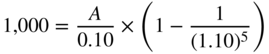
A = €315.47. Hence, the following repayment schedule:
| Period | Principal still due | Interest | Amortisation of principal | Annuity |
|---|---|---|---|---|
| 1 | 1,000 | 100 | 215.47 | 315.47 |
| 2 | 784.53 | 78.45 | 237.02 | 315.47 |
| 3 | 547.51 | 54.75 | 260.72 | 315.47 |
| 4 | 286.79 | 28.68 | 286.79 | 315.47 |
In this case, the interest for each period is indeed equivalent to 10% of the remaining principal (i.e. the nominal rate of return) and the loan is fully paid off in the fourth year. Internal rate of return and nominal rate of interest are identical, as calculation is on an annual basis and the repayment of principal coincides with the payment of interest.
Regardless of which side of the loan you are on, both work the same way. We start with invested (or borrowed) capital, which produces income (or incurs interest costs) at the end of each period. Eventually, the loan is then either paid back (leading to a decline in future revenues or in interest to be paid) or held on to, thus producing a constant flow of income (or a constant cost of interest).
4/ INTEREST AND PRINCIPAL BOTH PAID WHEN THE LOAN MATURES
In this case, the borrower pays nothing until the loan matures. The sum that the borrower will have to pay at maturity is none other than the future value of the sum borrowed, capitalised at the interest rate of the loan:
This is how the repayment schedule would look:
| Period | Principal and interest still due | Amortisation of principal | Interest payments | Annuity |
|---|---|---|---|---|
| 1 | 1,000 | 0 | 0 | 0 |
| 2 | 1,100 | 0 | 0 | 0 |
| 3 | 1,219 | 0 | 0 | 0 |
| 4 | 1,331 | 1,331 | 1,331 | 1,464.1 |
This is a zero-coupon loan.
SUMMARY
QUESTIONS
EXERCISES
ANSWERS
BIBLIOGRAPHY
NOTE
- 1 The formula for continuously compounded interest is t = ek − 1, where e stands for 2.71828 and k is an interest rate (10% in our example).