
![]()
Vector Spaces and Linear Applications. Equations and Systems
4.1 Matrix Algebra and Vector Spaces
Matrix algebra has a strong field of application in the theory of vector spaces, particularly in the study of types of linear transformations between vector spaces, linear forms, bilinear forms, quadratic forms, etc. It is also plays a critical role in the study of systems of linear equations.
The following MATLAB commands are useful when working in the above mentioned fields:
- nullspace (A) returns a basis for the kernel of A.
- N = null (A) generates an orthonormal basis for the kernel of A. The number of columns of N is the dimension of the kernel (the nullity) of A.
- Q = orth (A) generates an orthonormal basis for the range of A, i.e., the columns of Q generate the same space as the columns of A, and the number of columns in Q is the rank of A.
- colspace(A) returns a basis for the columns of A.
- dot (A, B) gives the dot product of vectors A and B.
- cross (A, B) gives the vector product of vectors A and B.
- subspace (A, B) finds the angle between two subspaces specified by the columns of A and B. If A and B are column vectors of unit length, this is the same as acos(abs(A’*B)).
- maple (‘kernel(A)’) or maple (‘nullspace (A)’) returns a basis for the kernel of A.
- maple (‘nullspace(A,n)’) or maple (‘kernel(A,n)’) returns a basis for the kernel of A and assigns to n the dimension of the kernel.
- maple (‘colspace(A)’) returns a basis for the columns of A.
- maple (‘colspace(A,n)’) returns a basis for the columns of A and assigns to n the dimension of the column space.
- maple (‘colspan(A)’) returns the generator set of vectors for the column space of the matrix A, whose elements can be multivariate polynomials over the rational numbers.
- maple (‘colspan(A,n)’) returns the generator set of vectors for the column space of the matrix A and assigns to n the dimension of the column space.
- maple (‘rowspace(A)’) returns a basis for the rows of the matrix A.
- maple (‘rowspace(A,n)’) returns a basis for the rows of A and assigns to n the dimension of the row space.
- maple (‘rowspan(A)’) returns a generator set of vectors for the row space of the matrix A, whose elements can be multivariate polynomials over the rational numbers.
- maple (‘rowspan(A,n)’) returns the generator set of vectors for the row space of the matrix A, and assigns to n the dimension of the row space.
- maple (‘dotprod(A, B)’) gives the dot product of vectors A and B.
- maple (‘dotprod(A,B,’orthogonal’)’) gives the dot product of vectors A and B in an orthogonal space.
- maple (‘crossprod(A, B)’) gives the vector product of vectors A and B.
- maple (‘innerprod (V1 A V2)’) computes the inner product of the vectors V1 and V2 and the matrix A.
- maple(‘innerprod(V1,A1,…,An,V2)’) calculates the inner product of the vectors V1 and V2 and the matrices A1, A2,…, An.
- maple (‘angle(A, B)’) gives the angle formed by the vectors A and B.
- maple (‘norm (V)’) returns the infinity norm of the vector V (the maximum of its elements).
- maple (‘norm(V, option)’) returns the norm of the vector V where the type of norm is specified by the option. Possible options are ‘infinity’, ‘frobenius’ or any positive integer. The Frobenius norm is the square root of the sum of squares of the components, the k-norm (positive integer k) is the kth root of the sum of the kth powers of the components.
- maple (‘normalize (V)’) normalizes the vector V (using the 2-norm of V).
- maple (‘basis({v1,v2,…,vn})’) gives a basis of the vector space generated by the set of vectors {v1, v2,…, vn}.
- maple (‘sumbasis({Vs1},{Vs2},…,{Vsn})’) gives a basis for the sum of the vector spaces generated by the sets of vectors {Vs1}, {Vs2},…, {Vsn}.
- maple(‘intbasis({Vs1},{Vs2},…,{Vsn})’) gives a basis for the intersection of the vector spaces generated by the sets of vectors {Vs1}, {Vs2},…, {Vsn}.
- maple(‘GramSchmidt({v1,v2,…,vn})’) uses the Gram–Schmidt process to create an orthogonal basis from the set of vectors {v1,v2,…,vn}. The basis does not have to be orthonormal.
4.2 Linear Independence, Bases, and Base Change
EXERCISE 4-1
Determine which of the following sets of vectors are linearly independent:
{{2,3,–1}, {0,0,1}, {2,1,0}}
{{1,2,–3,4},{3,–1,2,1},{1,–5,8,–7},{2,3,1,–1}}
{{1,2,2,1},{3,4,4,3},{1,0,0,1}}
>> A = [2,3,-1; 0,0,1; 2,1,0]
A =
2 3 -1
0 0 1
2 1 0
>> det(A)
ans =
4
Since the determinant is non-zero, the vectors are linearly independent.
>> B = [1,2,-3,4;3,-1,2,1;1,-5,8,-7;2,3,1,-1]
B =
1 2 -3 4
3 -1 2 1
1 -5 8 -7
2 3 1 -1
>> det(B)
ans =
0
Since the determinant is zero, the vectors are linearly dependent:
>> C = [1,2,2,1;3,4,4,3;1,0,0,1]
C =
1 2 2 1
3 4 4 3
1 0 0 1
>> rank(C)
ans =
2
As we have only three vectors in a space of dimension four, we cannot apply the determinant test, but they will be linearly independent if the rank of the corresponding matrix is 3. Since we see that the rank is 2, the vectors are linearly dependent.
EXERCISE 4-2
Find the dimension and a basis of the space generated by the following set of vectors:
{{2,3,4,–1,1},{3,4,7,–2,–1},{1,3,–1,1,8},{0,5,5,–1,4}}
The dimension of the space generated by a set of vectors is equal to the rank of the matrix formed by the vectors:
>> A = [2,3,4,-1,1;3,4,7,-2,-1;1,3,-1,1,8;0,5,5,-1,4]
A =
2 3 4 -1 1
3 4 7 -2 -1
1 3 -1 1 8
0 5 5 -1 4
>> rank(A)
ans =
3
The rank of the array is 3, so the requested dimension is 3.
To find a basis, we considered any non-singular matrix minor of order 3. The vectors containing components included in this minor will form a basis.
>> det([2,3,4;3,4,7;0,5,5])

ans =

-15
Then, a basis of the generated linear space is the set of vectors {{2,3,4,–1,1},{3,4,7,–2,–1},{0,5,5,–1,4}}.
A basis can be calculated directly in the following way:
>> pretty(sym(maple('basis({vector([2,3,4,-1,1]),vector([3,4,7,-2,-1]),
(((vector([1,3,-1,1,8]), vector ([0,5,5,-1,4])})')))
[2 3 4 -1 1]
[ ]
[3 4 7 -2 -1]
[ ]
[0 5 5 -1 4]
EXERCISE 4-3
Determine whether the set of vectors
{{2,3,–1}, {0,0,1}, {2,1,0}}
forms a basis of R3, and if so, find the components of the vector x = (3,5,1) with respect to this basis.
>> det([2,3,-1;0,0,1;2,1,0])
ans =
4
Since we have three vectors in a space of dimension 3, they will form a basis if the determinant of the corresponding matrix is non-zero. Thus, we see that they do indeed form a basis.
The components of the vector (3,5,1) with respect to this basis are found as follows:
>> inv([2,0,2;3,0,1;-1,1,0]) * [3,5,1]'
ans =
1.7500
2.7500
-0.2500
EXERCISE 4-4
Consider the bases B and B1 of three-dimensional real vector space R3:
B = {{1,0,0}, {–1, 1, 0}, {0,1,–1}}
B1 = {{1,0,–1}, {2,1,0}, {–1, 1, 1}}
Find the matrix for the change of basis B to B1 and calculate the components of the vector {2,1,3} in base B with respect to the basis B1.
>> B = [1,0,0;-1,1,0;0,1,-1];
>> B1 = [1,0,-1;2,1,0;-1,1,1];
>> A = inv(B1')*B'
A =
-0.5000 1.5000 2.5000
0.5000 -0.5000 -0.5000
-0.5000 1.5000 1.5000
>> sym (A)
ans =
[-1/2, 3/2, 5/2]
[ 1/2, -1/2, -1/2]
[-1/2, 3/2, 3/2]
We already have the change of basis matrix. Now we find the components of the B-vector [2,3,1] with respect to the basis B1.
>> sym(inv(B1')*B'*[2,1,3]')
ans =
[8]
[-1]
[5]
EXERCISE 4-5
Let V be a vector space of dimension 5 with basis B = {u1,…, u5}. Let L be the space generated by the vectors a1 = u1-u2 + 3u3 + 2u4 + 5u5, a2 = u1 + u2 + u3 + 2u4 + 3u5, a3 = u1 + u3-u4 + 2u5. Let M be the space generated by b1 = 13u1 + 2u2 + 3u3 + 8u4 + 8u5 and b2 = 17u1 + 3u2 + 3u3 + 10u4 + 9u5. Find a basis for L+M and another for L∩M.
The linear space L is generated by the vectors with components [1,–1, 3, 2, 5], [1,1,1,2,3] and [1,0,1,–1,2] with respect to the basis B. The space M is generated by the vectors with components [13,2,3,8,8] and [17,3,3,10,9] with respect to the basis B. We find a basis for L+M in the following way:
>> pretty(sym(maple('sumbasis({vector([1,-1,3,2,5]), vector([1,1,1,2,3]),
(((vector([1,0,1,-1,2])}, {vector([13,2,3,8,8]), vector([17,3,3,10,9])})')))
ans =
[17, 1, 1, 13]
[3, 0, 1, 2]
[3, 1, 1, 3]
[10 -1, 2, 8]
[9, 2, 3, 8]
Therefore the dimension of L+M is 4.
The above matrix columns form a basis of L+M. Now we calculate a basis for L∩M as follows:
>> pretty(sym(maple('intbasis({vector([1,-1,3,2,5]), vector([1,1,1,2,3]),
(((vector([1,0,1,-1,2])}, {vector([13,2,3,8,8]), vector([17,3,3,10,9])})')))
ans =
[-1]
[1]
[-3]
[-2]
[-5]
Therefore the dimension of L∩M is 4.
4.3 Vector Geometry in 2 and 3 Dimensions
EXERCISE 4-6
Normalize the vectors x1 = (1,1,–1) and x2 = (1, 1, 1), determine if they are orthogonal and find their vector product.
>> pretty(sym(maple('normalize(vector([1,1,-1]))')))
1/2 1/2 1/2
[1/3 3 1/3 3 - 1/3 3 ]
>> pretty(sym(maple('normalize(vector([1,1,1]))')))
1/2 1/2 1/2
[1/3 3 1/3 3 1/3 3 ]
The vectors are orthogonal if their scalar product is zero:
>> dot([1,1,-1],[1,1,1])
ans =
1
Thus, the vectors are orthogonal. We now calculate their vector product:
>> cross([1,1,-1],[1,1,1])
ans =
2 - 2 0
Thus, the vector product is the vector (2,–2, 0).
EXERCISE 4-7
Find the vector triple product of the vectors (1,1,2), (0,1,0), (0,1,1).
>> dot([1,1,2], cross ([0,1,0], [0,1,1]))
ans = 1
EXERCISE 4-8
Using the Gram-Schmidt process, find an orthogonal basis from the vectors (1,0,0), (1,1,0), (0,1,1).
>> maple('GramSchmidt ([vector([1,0,0]), vector([1,1,0]), vector([0,1,1])])')
ans =
[[1, 0, 0], [0, 1, 0], [0, 0, 1]]
EXERCISE 4-9
Find the area of the triangle whose vertices are at (0,0), (5,1) and (3,7).
>> (1/2) * det([0,0,1;5,1,1;3,7,1])
ans =
16
Here we have applied a well-known formula for the area of a triangle based on the coordinates of its vertices.
EXERCISE 4-10
Find the angle formed by the vectors a = (1,2,3) and b= (0,3,1).
>> pretty(sym(maple('angle([1,2,3],[0,3,1])')))
1/2 1/2
acos(9/140 14 10 )
Now, we approximate the result:
>> vpa(ans)
ans =
.7064997155064410
4.4 Linear Applications
EXERCISE 4-11
Given the linear transformation whose matrix is given by the set of vectors
{(0,–3,–1,–3,–1),(–3,3,–3,–3,–1),(2,2,–1,1,2)}
find a basis for its kernel. Also find the image of the vectors (4,2,0,0,–6) and (1,2, –1,–2, 3) under this linear transformation.
>> A = [0,-3,-1,-3,-1;-3,3,-3,-3,-1;2,2,-1,1,2]
A =
0 -3 -1 -3 -1
-3 3 -3 -3 -1
2 2 -1 1 2
>> null(A)
ans =
-0.5540 0
-0.3380 0.2236
-0.1828 0.6708
0.1584 -0.5814
0.7213 0.4025
The two columns of the previous output form a basis of the kernel of T, so the dimension of the kernel will be 2:
>> maple('T:=x->multiply(array([[0,-3,-1,-3,-1],[-3,3,-3,-3,-1],[2,2,-1,1,2]]),x)')
>> pretty(sym(maple('T([4,2,0,0,-6])')))
[0 0 0]
>> pretty(sym(maple('T([1,2,-1,-2,3])')))
[- 2 9 11]
EXERCISE 4-12
We consider the linear transformation f between two vector subspaces U and V such that f(e1) = v 1-v2, f(e2) = v2-v3 and f (e3) = v3-v4, where:
B = {e1, e2, e3} is a basis of U (a subspace of R3)
B' = {v1, v2, v3, v4} is a basis of V (a subspace of R4)
Find the matrix associated with the transformation f. Find the image of the vector v=(1,1,2) of U under the linear transformation f.
The matrix associated with f is evident, we need only examine the definition of f:
>> A = [1,0,0;-1,1,0;0,-1,1;0,0,1]
A =
1 0 0
-1 1 0
0 -1 1
0 0 1
>> maple('T1:=x->multiply(array([[1,0,0],[-1,1,0],[0,-1,1],[0,0,1]]),x)'),
>> pretty(sym(maple('T1([1,1,2])')))
[1 0 1 2]
EXERCISE 4-13
Consider the linear transformation f between two vector subspaces U and V of three-dimensional real space, so that f (a,b,c) = (a+b,b+c,a+c), for (a, b, c) in U.
Find the matrix associated to the transformations f, f5 and ef
>> maple('T:=(a,b,c)->[a+b,b+c,a+c]'),
To find the matrix of f, we will consider the image of the canonical basis vectors under the transformation f:
>> [maple('T(1,0,0)'), maple('T(0,1,0)'),maple('T(0,0,1)')]
ans =
[1, 0, 1] [1, 1, 0] [0, 1, 1]
The matrix whose columns are the above vectors is the matrix of the linear transformation f, which can be found directly via:
>> A = sym(maple('transpose(array([T(1,0,0),T(0,1,0),T(0,0,1)]))'))
A =
[1, 1, 0]
[0, 1, 1]
[1, 0, 1]
The matrix associated to f5 will be given by A5:
>> A ^ 5
ans =
11 10 11
11 11 10
10 11 11
The matrix associated to ef will be eA:
>> expm(A)
ans =
3.1751 2.8321 1.3819
1.3819 3.1751 2.8321
2.8321 1.3819 3.1751
EXERCISE 4-14
Consider the linear transformation f between two vector subspaces U (contained in R3) and V (contained in R4), so that f (a,b,c) = (a,0,c,0) for all (a, b, c) in U.
Find the matrix associated to the transformation f, its kernel and the dimensions of the kernel and the image of f.
>> maple('T:=(a,b,c)->[a,0,c,0]'),
>> A = sym(maple('transpose(array([T(1,0,0),T(0,1,0),T(0,0,1)]))'))
A =
[1, 0, 0]
[0, 0, 0]
[0, 0, 1]
[0, 0, 0]
The kernel is the set of vectors of U with null image in V:
>> null(A)
ans =
[0]
[1]
[0]
Thus the kernel will be the set of vectors (0,b,0), for b varying in U. In addition, the kernel obviously has dimension 1, since we have shown that a basis is given by the single vector (0,1,0):
>> maple('rank(matrix(4,3,[1,0,0,0,0,0,0,0,1,0,0,0]))')
ans =
2
The dimension of the image of f is 2, since the sum of the dimensions of the kernel and the image must be the dimension of U (which is 3). On the other hand, the dimension of the image of f must match the rank of the matrix of the linear transformation, which is 2. Two column vectors containing the elements of a non-singular minor of the matrix of f will form a basis of the image of f:
>> det([1,0;0,1])
ans =
1
Thus, a basis of the image of f will be {(1,0,0,0),(0,0,1,0)}.
EXERCISE 4-15
Consider the bilinear form f:U×V - > R, where U and V are two vector subspaces of three-dimensional real space R3, such that:
f [{(x1, x2, x3), (y1, y2, y3)}] = x1 y1-2x1 y2 + 4x2 y3 - x3 y1-3 x3 y3
Find the matrix associated with the bilinear form f and classify it.
>> maple('A:=array([[1,-2,0],[0,0,4],[-1,0,-3]])'),pretty(sym(maple('A')))
[ 1 -2 0]
[ ]
[ 0 0 4]
[ ]
[-1 0 -3]
>> pretty(expand (sym (maple ('evalm ([[x 1, x 2, x 3]] & * A & * transpose([[y1, y2, y3]]))')));)
y1 x1 - y1 x3 - 2 x1 y2 + 4 y3 x2-3 x3 y3
Then, the f matrix is {{1, –2, 0}, {0,0,4}, {–1, 0, –3}}.
maple('det (A)'),
8
As the determinant of the matrix of f is non-zero, the bilinear form is regular non-degenerate.
4.5 Quadratic Forms
EXERCISE 4-16
Consider the quadratic form f: U→R, where U is a vector subspace of real three-dimensional space R3, such that:
f [(x,y,z)] = x2 – 2xy + y2 + 6xz – 3yz + 4z2
Find the matrix associated with f and classify it.
>> maple('A:=array([[1,-1,3],[-1,1,-3/2],[3,-3/2,4]])'),pretty(sym(maple('A')));
[ 1 -1 3 ]
[ ]
[-1 1 -3/2]
[ ]
[ 3 -3/2 4 ]
>> pretty(simplify(sym(maple('evalm([[x, y, z]] & * A & * transpose ([[x, y, z]]))'))))
2 2 2
x - 2 x y + 6 x z + y - 3 y z + 4 z
Thus, A is the matrix associated with f.
To classify it, we find the corresponding determinants.
>> pretty(sym(maple('det(A)')));
-9/4
>> pretty(sym(maple('det([[1,-1],[-1,1]])')));
0
The quadratic form is negative semidefinite.
However, we can also obtain the classification via the eigenvalues of the matrix of the quadratic form.
A quadratic form is defined to be positive definite if and only if all its eigenvalues are strictly positive. A quadratic form is defined to be negative definite if and only if all its eigenvalues are strictly negative.
A quadratic form is positive semidefinite if and only if all its eigenvalues are non-negative. A quadratic form is negative semidefinite if and only if all its eigenvalues are not positive.
A quadratic form is indefinite if it has both positive and negative eigenvalues.
>> pretty(sym(maple('evalf(eigenvals(A))')))
-31
6.4498046649069250305217677941300 +.2 10 i,
-31
-.85690615612023945647201856979180 -.1 10 i,
-31
.40710149121331442595025077566180 -.1 10 i
All of the eigenvalues are complex, so the quadratic form is indefinite.
EXERCISE 4-17
Consider the quadratic form f: U→R, where U is a vector subspace of real three-dimensional space R3, such that:
f [(x, y, z)] = x2 + 2y2 + 4yz + 2z2
Find the matrix associated with f and classify it. Find its reduced form, its rank and its signature.
>> maple('A:=array([[1,0,0],[0,2,2],[0,2,2]])'),pretty(sym(maple('A')))
[1 0 0]
[ ]
[0 2 2]
[ ]
[0 2 2]
>> pretty(simplify(sym(maple('evalm([[x, y, z]] & * A & * transpose ([[x, y, z]]))'))))
2 2 2
x + 2 y + 4 y z + 2 z
Thus, the matrix of the quadratic form is the matrix A.
>> pretty(sym(maple('det(A)')))
0
>> pretty(sym(maple('det([[1,0],[0,2]])')))
2
The quadratic form is degenerate positive semidefinite.
To find the reduced form, we diagonalize the matrix:
>> pretty(sym(maple('jordan(A)')))
[0 0 0]
[ ]
[0 1 0]
[ ]
[0 0 4]
>> pretty(sym(maple('evalm([[a, b, c]] & * jordan (A) & * transpose ([[a, b, c]]))')))
2 2
a + 4 c
Thus, the reduced form is given by f(a,b,c) = a2 + 4c2.
>> pretty(sym(maple('rank(jordan(matrix(3,3,[1,0,0,0,2,2,0,2,2])))')))
2
The rank of the quadratic form is 2, since the rank of the matrix is 2. The signature is also 2, since the number of positive terms in the diagonal of the diagonal matrix is 2.
4.6 Equations and Systems
MATLAB offers certain commands that allow you to solve equations and systems. Among them are the following:
- solve(‘equation’, ‘x’) solves the equation with respect to the variable x.
- syms x; solve(equ(x), x) solves the equation equ(x) with respect to the variable x.
- solve(‘eq1,eq2,…,eqn’, ‘x1,x2,…,xn’) solves the simultaneous equations eq1,…,eqn (in terms of the system variables x1,…, xn).
- syms x1 x2 … xn ; solve(eq1, eq2, …, eqn, x1, x2, …, xn) solves the simultaneous equations eq1,…,eqn (in terms of the system variables x1,…, xn).
- X = linsolve(A,B) solves A * X = B for a square matrix A, and matrices B and X.
- x = nnls (A, b) solves A * X = b using the method of least squares, where x is a vector (x ≥ 0).
- x = lscov(A,b,V) gives the vector X that minimizes (A * x–b)’* inv (V) *(A*x–b).
- roots(V) gives the roots of the polynomial whose coefficients are the components of the vector V.
- X = AB solves the system A * X = B.
- X = A/B solves the system X * A = B.
In addition, equations and systems of equations can be solved using the following commands (all of them must be preceded by the maple command):
- solve(equation, variable) solves the given equation for the given variable.
- solve (expression, variable) solves the equation expression = 0 for the given variable.
- solve({expr1,..,exprn},{var1,..,varn}) solves the given system of equations for the specified variables.
- solve(equation) solves the equation for all of its variables.
- solve(expr1,…,exprn) solves the system specified by the equations for all possible variables.
- solve(inequal, variable) solves the inequality for the specified variable.
- solve(s, var) solves the equation in the series s for the specified variable.
- subs(solutions, equations) substitutes the given list of solutions into the equations, to verify solutions.
- lhs (equation) returns the left-hand side of the equation.
- lhs (inequality) returns the left-hand side of the inequality.
- rhs (equation) returns the right-hand side of the equation.
- rhs (inequality) returns the right-hand side of the inequality.
- readlib (isolate): isolate (equation, expression) isolates the expression in the equation and attemtps to solve for it.
- readlib (isolate): isolate (expr1, expr2) equivalent to isolate (expr1=0, expr2).
- reablib (isolate): isolate (equation, expression, n) The integer n controls the maximum number of transformation steps that isolate performs. The default is 100000.
- testeq(expr1=expr2) or testeq (expr1, expr2) tests if the expressions are equivalent. The purpose may be to eliminate redundant equations in a system.
- eliminate (setequ, setvar) eliminates the given set of variables in the set of specified equations.
- isolve (equation) gives the integer solutions of the given equation for all of its variables.
- isolve (expression) gives the integer solutions of the equation expression = 0 for all of its variables.
- isolve({equ1,..,equn}) gives the integer solutions to the specified system of equations for all variables.
- isolve (equation, variable) gives the integer solutions of the specified equation in the given variable.
- isolve({equ1,…,equn},{var1,…,varn}) gives the integer solutions of the specified system in the given variables.
- isolve(equation,{var1,…,varn}) gives the integer solutions of the specified equation in the given variables.
- fsolve (equation, variable) solves the given equation using Newton’s method.
- fsolve (expression, variable) solves the equation expression = 0 in the given variable using Newton’s method.
- fsolve ({equ1,…,equn},{var1,…,varn}) solves the system of equations for the given variables using numerical methods (the number of equations equals the number of unknowns).
- fsolve (expr) or fsolve({equ1,…,equn}) solves the equation expr = 0 for the system using numerical methods.
- fsolve (equation,var,a..b) solves the equation in the variable var by numerical methods, obtaining solutions in the interval [a, b].
- fsolve ({equ1,…,equn},{var1,…,varn},{var1=a1..b1,…, varn = an…bn}) finds real solutions of the system in the given variables that are in the specified intervals (by numerical methods).
- fsolve (equation, variable, complex) finds the complex solutions of the given equation.
- fsolve (equation,variable,‘maxsols’=m) finds up to m solutions of the given equation.
- fsolve (equation, variable, ‘fulldigits’) ensures an optimum value of Digits in order to compute the largest number of possible solutions of the given equation in the specified variable.
- msolve(equation, m) solves the equation modulo m in all its variables.
- msolve(expression, m) solves the equation expression = 0 modulo m in all its variables.
- msolve({equ1,…,equn},m) solves the given system modulo m in all its variables.
- msolve(equation,variable,m) or msolve(equation,{var1,…,varn},m) solves the equation modulo m in the variable or variables specified.
- msolve({equ1,…,equn},{var1,…,varn},m) solves the given system modulo m in the specified variables.
- RootOf (equation, variable) represents the roots of the given equation in the specified variable in the form of RootOf expressions. For certain equations it is only possible to express the solutions in terms of RootOf expressions.
- RootOf (expression, variable) presents the solutions of the equation expression = 0 in terms of RootOf expressions.
- RootOf (equation) presents the solutions of the given univariate equation in terms of RootOf expressions.
- allvalues (expr) Expressions involving RootOfs often evaluate to more than one value or expression. The allvalues command returns all possible values. It uses solve to calculate the exact roots of the expression, and if this is impossible, it uses fsolve to calculate the approximate solutions.
- allvalues(expr,d) indicates that identical RootOfs in the expression are only to be evaluated once, thus avoiding redundancy and reducing the calculation time.
- convert (ineq, equality) converts the given inequality to an equation by replacing the symbols < or < = by =.
- convert (equ, lessequal) converts the given equation or strict inequality to a non-strict inequality replacing the symbols < or = by < =.
- convert (equ, lessthan) converts the given equation or non-strict inequality to the corresponding strict inequality replacing the symbols = or < = by the symbol <.
- with(student):equate(list1,list2) creates a set of equations of the form {list1[1] = list2[1],…, list1[n] = list2[n]}.
- equate(list) creates a set of equations of the form {list [1] = 0,…, list [n] = 0}.
- equate (array1, array2) converts the two arrays to a set of equations.
- equate (table1, table2) converts the two tables to a set of equations.
- equate (expr1, expr2) converts the two expressions to the set containing the equation expr1 = expr2.
Here are some examples:
First, we solve an equation in exact and approximate form and check one of the solutions.
>> pretty(sym(maple('eq := x^4-5*x^2+6*x=2: solve(eq,x)')))

                                1/2        1/2
                          -1 + 3   , -1 - 3   , 1, 1

>> pretty(sym(maple('sols := [solve(eq,x)] : evalf(sols,10)')))

                   [.732050808    -2.732050808    1.    1.]

>> pretty(simple(sym(maple('subs( x=sols[1], eq )'))))

                                     2 = 2
The above equation also can be solved as follows:
>> solve('x^4-5*x^2+6*x=2')

ans =

[- 1 + 3 ^(1/2)]
[- 1 - 3 ^(1/2)]
[             1]
[             1]
Another way to solve the same equation would be as follows:
>> syms x
>> solve(x^4-5*x^2+6*x-2)

ans =

[- 1 + 3 ^(1/2)]
[- 1 - 3 ^(1/2)]
[             1]
[             1]
Next we solve a system of equations and check their solutions.
>>  maple('eqns:= {u+v+w=1, 3*u+v=3, u-2*v-w=0}:sols:= solve(eqns)')

ans =

sols: = {w = -2/5, v = 3/5, u = 4/5}

>> maple('subs( sols, eqns )')

ans =

{1 = 1, 0 = 0, 3 = 3}
The previous system also can be solved in the following way:
>> syms u v w
>> [u, v, w] = solve(u+v+w-1, 3*u+v-3, u-2*v-w, u,v,w)

u =

4/5

v =

3/5

w =

-2/5
Alternatively, we can solve the system as follows:
>> [u, v, w] = solve('u+v+w=1', '3*u+v=3', 'u-2*v-w=0', 'u','v','w')

u =

4/5

v =

3/5

w =

-2/5
Or we can do the following:
>> [u, v, w] = solve('u+v+w=1, 3*u+v=3, u-2*v-w=0', 'u,v,w')

u =

4/5

v =

3/5

w =

-2/5
Next we solve some systems subject to certain conditions.
>> pretty(sym(maple('solve({x^2*y^2=0, x-y=1})')))

   {x = 0, y = - 1}, {x = 0, y = - 1}, {x = 1, y = 0}, {x = 1, y = 0}

>> pretty(sym(maple('solve({x^2*y^2=0, x-y=1, x<>0}) ')))

                    {x = 1, y = 0}, {x = 1, y = 0}

>> pretty(sym(maple('solve({x^2*y^2-b, x^2-y^2-a}, {x,y}) ')))

{y = 1/2 %4, x = 1/2 %3}, {y = 1/2 %4, x = - 1/2 %3},

    {y = - 1/2 %4, x = 1/2 %3}, {y = - 1/2 %4, x = - 1/2 %3},

    {y = 1/2 %1, x = 1/2 %2}, {x = - 1/2 %2, y = 1/2 %1},

    {y = - 1/2 %1, x = 1/2 %2}, {x = - 1/2 %2, y = - 1/2 %1}}

                    2      1/2 1/2
%1: = (- 2 a - 2 (a + 4 (b) ) )

                 2       1/2 1/2
%2: = (2 a - 2 (a + 4 (b) ) )

               2      1/2  1/2
3%: = (2 + 2 (a + 4 (b) ) )

                   2       1/2 1/2
%4: = (- 2 a + 2 (a + 4 (b) ) )
Now we find the integer solutions of an equation.
>> pretty(sym(maple('isolve(3*x-4*y=7) ')))

                    {y = 2 + 3 _N1, x = 5 + 4 _N1}
We solve a system and an equation approximately.
>> maple('f: = sin(x + y) - exp(x) * y = 0: ' g: = x ^ 2 - y = 2: '),
>> pretty(sym(maple('fsolve({f,g},{x,y},{x=-1..1,y=-2..0}) ')))

                 {y = -1.552838698, x = -.6687012050}

>> maple('f: = 10-(ln(v+(v^2-1)^(1/2))-ln(3+(3^2-1)^(1/2)))') ;

>> pretty(sym(maple('fsolve(f,v)')))

                             64189.82535

>> pretty(sym(maple('fsolve(f,v,1..infinity)')))

                            64189.82535
In the two following equations, instead of isolating x, we isolate sin (x) in the first equation and x2 in the second equation.
>> pretty(sym(maple('readlib(isolate):isolate(4*x*sin(x)=3,sin(x))')))

                           sin (x) = 3/4 x

>> pretty(sym(maple('isolate(x^2-3*x-5,x^2) ')))

                              2
                             x = 3 x + 5
We now verify that two expressions are not equal, but are probabilistically equivalent.
>> maple('a: = (sin (x) ^ 2 - cos (x) * tan (x)) * (sin (x) ^ 2 + cos (x) * tan (x)) ^ 2:)
   b: = 1/4 * sin(2*x) ^ 2 - 1/2 * sin(2*x) * cos (x) - 2 * cos (x) ^ 2
          + 1/2 * sin(2*x) * cos (x) ^ 3 + 3 * cos (x) ^ 4 - cos (x) ^ 6:'),

>> pretty(sym(maple('evalb( a = b ) ')))

                               false

>> pretty(sym(maple('evalb( expand(a) = expand(b) )')))

                                false

>> pretty(sym(maple('testeq( a = b )')))

                                true
In the following example, we eliminate a variable from a system:
>> pretty(sym(maple('readlib(eliminate): eliminate({x ^ 2 + y ^ 2-1, x ^ 3 - y ^ 2 * x + x * y-3}, x)')))

                3          6      4     5     3     2
 [{x = - -----------}, {4 y - 7 y - 4 y + 6 y + 4 y - 2 y + 8}]
            2
         2 y - y - 1
EXERCISE 4-18
Find the solutions to the following equations:
sin(x) cos(x) = 0, sin(x) = acos(x), ax ^ 2 + bx + c = 0 and sin(x) + cos(x) = sqrt(3)/2.
>> solve('sin(x) * cos(x) = 0')
ans =
[ 0]
[1/2 * pi]
[-1/2 * pi]
>> solve('sin(x) = a * cos(x) ',' x')
ans =
atan (a)
>> solve('a*x^2+b*x+c=0','x')
ans =
[1/2/a * (-b + (b ^ 2-4 * a * c) ^(1/2))]
[1/2/a * (-b-(b^2-4*a*c) ^(1/2))]
>> solve('sin(x)+cos(x)=sqrt(3)/2')
ans =
[1/2 * 3 ^(1/2)]
[1/2 * 3 ^(1/2)]
EXERCISE 4-19
Find at least two solutions of each of the following two trigonometric and exponential equations:
![]()
First, we use the command fsolve:
>> maple('fsolve(x * sin (x) = 1/2)')
ans =
-.74084095509549062101093540994313
>> maple('fsolve(2^(x^3)=4*2^(3*x))')
ans =
2.0000000000000000000000000000000
For both equations we get a single solution. To find more solutions, we graph the functions to find approximate intervals where possible solutions might fall. See Figure 4-1:
>> fplot('[x * sin(x) - 1/2.0]', [0, 4 * pi])
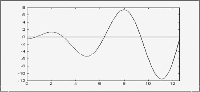
We observe that there is a solution between 0 and 2, another between 2 and 4, another between 4 and 8, and so on. We can calculate three of them:
((' s1=maple('fsolve(x*sin(x)=1/2,x,0..2)')
s1 =
.7408409550954906
>> s2=maple('fsolve(x*sin(x)=1/2,x,2..4)')
s2 =
2.972585490382360
>> s3=maple('fsolve(x*sin(x)=1/2,x,4..8)')
S3 =
6.361859813361645
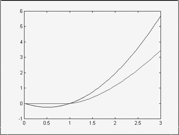
We repeat this process for the second equation, starting with the graph (see Figure 4-2):
>> subplot(2,1,1)
>> fplot('[2^(x^3),4*2^(3*x)]',[-3,1,-1/4,3/2])
>> subplot(2,1,2)
>> fplot('[2^(x^3),4*2^(3*x)]',[1,3,100,400])

Two parts of the graph are shown where there are intersections. There are possible solutions between –4 and 0, and between 0 and 3. Given this information we try to calculate these solutions:
>> maple('fsolve(2 ^(x^3) = 4 * 2 ^(3*x), x, - 4.. 0)')
ans =
-1.00000000000
>> maple('fsolve(2^(x^3)=4*2^(3*x),x,0..3)')
ans =
2.00000000000
We see that x = –1 and x = 2 are exact solutions of the equation.
EXERCISE 4-20
Solve each of the following two logarithmic and surd equations:
x3/2 log(x) = x log(x3/2), sqrt[1-x]+sqrt[1+x] = a.
>> maple('fsolve(x^(3/2)*log(x)=x*log(x)^(3/2))')
ans =
1.
Next we graph the function (see Figure 4-3) in order to find the intervals in which possible solutions may be found. This confirms that x = 1 is the only real solution.
>> fplot('[^(3/2) x * log(x), x * log(x) ^(3/2)]', [0.3, -1, 6])
Now, let’s solve the surd equation:
>> pretty(sym(solve('sqrt(1-x)+sqrt(1+x)=a','x')))
2 1/2
[-1/2 a (-a + 4) ]
[ ]
[ 2 1/2 ]
[1/2 a (-a + 4) ]
EXERCISE 4-21
Solve the following two equations:
x5 + 16x4 + 7x3+ 17x2 + 11x + 5 = 0 and x4 – 1 = 0.
In addition, solve the first equation modulo 19 and the second modulo 5.
>> s1=solve('x^5 +16*x^4+7*x^3+17*x^2+11*x+5=0')
[ -15.61870451719182]
[-.3867059805744952-.3977796861292117*i]
[-.3867059805744952+.3977796861292117*i]
[ .1960582391704047-1.000858165543796*i]
[ .1960582391704047+1.000858165543796*i]
>> s2=solve('x^4-1=0')
s2 =
[1]
[-1]
[i]
[-i]
Now we find the modulo 19 solutions of the first equation:
>> maple('msolve(x^5 +16*x^4+7*x^3+17*x^2+11*x+5=0,19)')
ans =
{x = 1}, {x = 18}, {x = 3,} {x = 7}, {x = 12}
We calculate the modulo 5 solution of the second equation:
>> maple('msolve(x^4-1=0,5)')
ans =
{x = 1}, {x = 2}, {x = 3,} {x = 4}
Since the two equations are polynomial equations, we also have the option to solve them with the command roots. We have:
>> roots([5,11,17,7,16,5])
ans =
-1.2183 + 1.3164i
-1.2183 - 1.3164i
0.2827 + 0.9302i
0.2827 - 0.9302i
-0.3289
>> roots([-1,0,0,0,1])
ans =
-1.0000
0.0000 + 1.0000i
0.0000 - 1.0000i
1.0000
EXERCISE 4-22
Solve the following system of two equations:

>> [x, y] = solve('cos(x/12) /exp(x^2/16) = y ',' - 5/4 + y = sin(x ^(3/2))')
x =
2.412335896593778
y =
.6810946557469383
EXERCISE 4-23
Find the intersection of the hyperbolas with equations x2 – y2 = r2 and a2x2 – b2y2 = a2b2 with the parabola z2 = 2px.
>> [x, y, z] = solve('a^2*x^2-b^2*y^2=a^2*b^2','x^2-y^2=r^2','z^2=2*p*x', 'x,y,z')
x =
[1/2*RootOf((a^2-b^2)*_Z^4+4*b^2*r^2*p^2-4*a^2*b^2*p^2)^2/p]
[1/2*RootOf((a^2-b^2)*_Z^4+4*b^2*r^2*p^2-4*a^2*b^2*p^2)^2/p]
y =
[1/2*(RootOf((a^2-b^2)*_Z^4+4*b^2*r^2*p^2-4*a^2*b^2*p^2)^4-4*r^2*p^2)^(1/2)/p]
[-1/2*(RootOf((a^2-b^2)*_Z^4+4*b^2*r^2*p^2-4*a^2*b^2*p^2)^4-4*r^2*p^2)^(1/2)/p]
z =
[RootOf((a^2-b^2)*_Z^4+4*b^2*r^2*p^2-4*a^2*b^2*p^2)]
[RootOf((a^2-b^2)*_Z^4+4*b^2*r^2*p^2-4*a^2*b^2*p^2)]
Now, we simplify the RootOf expression:
>> [simple(allvalues (x)), simple(allvalues (y)), simple(allvalues (z))]
ans =
[b*(-r^2+a^2) ^(1/2) /(a^2-b^2) ^(1/2) b] [a *(b^2-r^2) ^(1/2) /(a^2-b^2) ^(1/2)] [2 ^(1/2) * b ^(1/2) * p ^(1/2) *(-r^2+a^2) ^(1/4) /(a^2-b^2) ^(1/4)]
[b*(-r^2+a^2) ^(1/2) /(a^2-b^2) ^(1/2) b] [a *(b^2-r^2) ^(1/2) /(a^2-b^2) ^(1/2)] [- 2 ^(1/2) * b ^(1/2) * p ^(1/2) *(-r^2+a^2) ^(1/4) /(a^2-b^2) ^(1/4)]
[-b *(-r^2+a^2) ^(1/2) /(a^2-b^2) ^(1/2)] [a *(b^2-r^2) ^(1/2) /(a^2-b^2) ^(1/2)] [i * 2 ^(1/2) * b ^(1/2) * p ^(1/2) *(-r^2+a^2) ^(1/4) /(a^2-b^2) ^(1/4)]
[-b*(-r^2+a^2)^(1/2)/(a^2-b^2)^(1/2)] [ a*(b^2-r^2)^(1/2)/(a^2-b^2)^(1/2)] [-i*2^(1/2)*b^(1/2)*p^(1/2)*(-r^2+a^2)^(1/4)/(a^2-b^2)^(1/4)]
[ b*(-r^2+a^2)^(1/2)/(a^2-b^2)^(1/2)] [-a*(b^2-r^2)^(1/2)/(a^2-b^2)^(1/2)] [ 2^(1/2)*b^(1/2)*p^(1/2)*(-r^2+a^2)^(1/4)/(a^2-b^2)^(1/4)]
[ b*(-r^2+a^2)^(1/2)/(a^2-b^2)^(1/2)] [-a*(b^2-r^2)^(1/2)/(a^2-b^2)^(1/2)] [ -2^(1/2)*b^(1/2)*p^(1/2)*(-r^2+a^2)^(1/4)/(a^2-b^2)^(1/4)]
[-b*(-r^2+a^2)^(1/2)/(a^2-b^2)^(1/2)] [-a*(b^2-r^2)^(1/2)/(a^2-b^2)^(1/2)] [ i*2^(1/2)*b^(1/2)*p^(1/2)*(-r^2+a^2)^(1/4)/(a^2-b^2)^(1/4)]
[-b*(-r^2+a^2)^(1/2)/(a^2-b^2)^(1/2)] [-a*(b^2-r^2)^(1/2)/(a^2-b^2)^(1/2)] [-i*2^(1/2)*b^(1/2)*p^(1/2)*(-r^2+a^2)^(1/4)/(a^2-b^2)^(1/4)]
Each line of this output (triple of values) is a solution of the system, i.e., a point of intersection of the three curves.
EXERCISE 4-24
Solve the inequality x2 + x > 5.
>> maple('solve(x^2+x>5,x)')
ans =
RealRange(-inf,Open(-1/2-1/2*21^(1/2))),RealRange(Open(-1/2+1/2*21^(1/2)),inf)
4.7 Systems of Linear Equations
In the previous sections we have studied equations and systems in general. We will now focus on linear systems of equations. To solve such systems we could simply use the commands we have seen so far, however MATLAB has a selection of special commands designed especially for linear systems. We summarize these commands below.
- linsolve(M,V) solves the system M&*x=V, where M is the matrix of the system and V is the vector of independent terms (number of elements of V = number of rows in M).
- linsolve (M1, M2) finds the matrix X such that M1&*X=M2. The dimensions of M1, M2 and X must be compatible.
- linsolve(M,V,name,variable) solves the system M&*x = V and assigns the specified name to the rank of M. If Maple needs to name variables for solutions it will use the names variable[1], variable[2], etc. If the variable argument is not specified, Maple will use values _t[1], _t[2], etc. as variable names, if necessary.
- leastsqrs(M,V) finds the vector x satisfying the equation M&*x=V in the sense of least squares (x minimizes the 2-norm of M &*x--V).
- leastsqrs({equ1,…,equm},{var1,…,varn}) gives var1,…, varn that satisfies the given system of equations equ1,…, equm in the least squares sense.
Systems of linear equations can be converted to array form and solved using calculations with matrices. A system can be written in the form M.X = B, where X is the vector of variables, B the vector of independent terms and M the matrix of coefficients of the system. If M is a square matrix and the determinant of the matrix M is non-null, M is invertible, and the unique solution of the system can be written in the form: X = M-1B. In this case, the commands solve, linsolve, lscov, bicg, pcg, lsqr, gmr, gmres, minres, symmlq or MB, already described above, offer the solution.
If the determinant of M is zero, the system has infinitely many solutions, since there are rows or columns in M that are linearly dependent. In this case, the number of redundant equations can be calculated to find out how many variables are needed to describe the solutions. If the matrix M is rectangular (not square), the system may be undetermined (the number of equations is less than the number of variables), overdetermined (the number of equations is greater than the number of variables) or non-singular (the number of equations is equal to number of variables and M has non-zero determinant). An indeterminate system can have infinitely many solutions, or none, and likewise for an overdetermined system. If a system has no solution, it is called inconsistent (incompatible), and if there is at least one solution, it is called consistent (compatible). The system M . X = B is called homogeneous when the vector B is the null vector, i.e. the system is of the form M . X= 0. If the determinant of M is non-null, the unique solution of the system is the null vector (obtained with the command linsolve). If the determinant of M is zero, the system has infinitely many solutions. The solutions can be found using the commands solve, linsolve, lsqr or other commands described above for general linear systems.
Below is an example of a system with infinitely many solutions: (x + 3y + 4z = 1, 2x + 3y + 3z = 1). In this case, MATLAB describes a parameterization of these solutions:
>> maple('solve({x+3*y+4*z=1, 2*x+3*y+3*z=1},{x,y,z})')

ans =

y = - 5/3 * z + 1/3, x = z, z = z
Any value of z will yield a solution of the system.
4.8 The Rouche-Frobenius Theorem
A fundamental tool in the analysis and solution of systems of equations is the Rouche-Frobenius theorem. This theorem says that a system of m equations with n unknowns has a solution if, and only if, the rank of the matrix of coefficients coincides with the rank of the array extended with the vector column of the system-independent terms. If the two ranks are equal, and equal to the number of unknowns, the system has a unique solution. If the two ranks are the same, but less than the number of unknowns, the system has infinitely many solutions. If they are different, the system has no solution.
In summary: Let A be the matrix of coefficients of the system and B the matrix A augmented by the column vector of independent terms.
If rank(A)1 rank(B), the system is incompatible (without solution).
If rank (A) = rank(B) < n, the system is indefinite (has infinitely many solutions).
If = rank(A) = rank(B) = n, the system has a unique solution.
This theorem allows us to analyze the solutions of a system of equations before solving it.
EXERCISE 4-25
Study and solve the system:
2x1 + x2 + x3 + x4 = 1
x1 + 2x2 + x3 + x4 = 1
x1 + x2 + 2 x3 + x4 = 1
x1 + x2 + x3 + 2x4 = 1
>> A = [2,1,1,1;1,2,1,1;1,1,2,1;1,1,1,2]
A =
2 1 1 1
1 2 1 1
1 1 2 1
1 1 1 2
>> B = [2,1,1,1,1;1,2,1,1,1;1,1,2,1,1;1,1,1,2,1]
B =
2 1 1 1 1
1 2 1 1 1
1 1 2 1 1
1 1 1 2 1
>> [rank(A), rank(B)]
ans =
4 4
We see that the matrix A and its augmented matrix B have rank 4, which, moreover, coincides with the number of unknowns. Therefore, the system has a unique solution. To calculate the solution, we use, for example, the command linsolve:
>> b = [1,1,1,1];
>> linsolve(A, b)
ans =
[1/5]
[1/5]
[1/5]
[1/5]
EXERCISE 4-26
Study and solve the system:
x1 – x2 + x3 = 1
4x1 + 5x2 – 5x3 = 4
2x1 + x2 – x3 = 2
x1 + 2x2 – 2x3 = 1
>> A = [1,-1,1;4,5,-5;2,1,-1;1,2,-2]
A =
1 -1 1
4 5 -5
2 1 -1
1 2 -2
>> B = [1,-1,1,1;4,5,-5,4;2,1,-1,2;1,2,-2,1]
B =
1 -1 1 1
4 5 -5 4
2 1 -1 2
1 2 -2 1
>> [rank(A), rank(B)]
ans =
2 2
We see that the rank of A and B coincide and its value is 2, which is less than the number of unknowns in the system (3). Therefore, the system will have infinitely many solutions. We try to solve it with the command solve:
>> maple('solve({x1-x2+x3=1,4*x1+5*x2-5*x3=4,2*x1+x2-x3=2,))
x1+2*x2-2*x3=1}, {x1,x2,x3})')
ans =
{x 2 = x 3, x 1 = 1, x 3 = x 3}
Infinitely many solutions are obtained using the parameter x3, so that the set of solutions is given by {(1, x3, x3): x3∈R}. Note that the trivial solution (1,0,0) is obtained by setting the parameter equal to zero.
The solution can also be found with the command leastsqrs as follows:
>> pretty(sym(maple('leastsqrs(array([[1,-1,1],[4,5,-5],[2,1,-1],[1,2,-2]]),
vector([1,4,2,1]))')))
1, _t [1], _t [1]
EXERCISE 4-27
Study and solve the system:
x + 2y + 3z = 6
x + 3y + 8z = 19
2x + 3y + z = –1
5x + 6y + 4z = 5
>> A = [1,2,3;1,3,8;2,3,1;5,6,4]

A =

1     2     3
1     3     8
2     3     1
5     6     4

>> B = [1,2,3,6;1,3,8,19;2,3,1,-1;5,6,4,5]

B =

1     2     3     6
1     3     8    19
2     3     1    -1
5     6     4     5

>> [rank(A), rank(B)]

ans =

3 3
We see that the ranks of A and B coincide and its value is 3, which is equal to the number of unknowns in the system. Therefore the system will have a unique solution. The only solution is obtained with the command linsolve:
>> maple('solve({x+2*y+3*z=6,x+3*y+8*z=19,2*x+3*y+z=-1, 5*x+6*y+4*z=5}, {x,y,z})')
ans =
x = 1, y = - 2, z = 3
The solution also can be found with the command linsolve as follows:
>> pretty(sym(maple('linsolve(array([[1,2,3],[1,3,8],[2,3,1],[5,6,4]]),
(((vector([6,19,-1,5]))')))
[1 -2 -3]
EXERCISE 4-28
Study and solve the system:
x + 2y + 3z + t = 6
x + 3y + 8z + t = 19
>> A = [1,2,3,1;1,3,8,1]
A =
1 2 3 1
1 3 8 1
>> B = [1,2,3,1,6;1,3,8,1,19]
B =
1 2 3 1 6
1 3 8 1 19
>> [rank(A), rank(B)]
ans =
2 2
We see that the rank of A and B coincide and its value is 2, which is less than the number of unknowns in the system (4). Therefore, the system has infinitely many solutions. We try to solve it:
>> maple('solve({x+2*y+3*z+t=6,x+3*y+8*z+t=19},{x,y,z,t})')
ans =
{y = - 5 * z + 13, t = - x+7 * z-20, x = x, z = z}
This time the solution depends on two parameters. As z and t vary over the real numbers, all the solutions of the system are obtained. These solutions form a two-dimensional subspace of four-dimensional real space.
The solution can also be found with the commands leastsqrs and linsolve as follows:
>> pretty(sym(maple('linsolve(array([[1,2,3,1],[1,3,8,1]]),vector([6,19]))')))
[_t[2], 13 - 5 _t[1], _t[1], -_t[2] - 20 + 7 _t[1]]
>> pretty(sym(maple('leastsqrs(array([[1,2,3,1],[1,3,8,1]]),vector([6,19]))')))
[_t [2], 13 - 5 _t [1], _t [1], - _t [2] - 20 + 7 _t [1]]
EXERCISE 4-29
Study and solve the system:
x1 + 2x2 – x3 = 10
2x1 + 4x2 – 2x3 = 5
x1 + x2 + x3 = 6
>> A = [1,2,-1;2,4,-2;1,1,1]
A =
1 2 -1
2 4 -2
1 1 1
>> B = [1,2,-1,10;2,4,-2,5;1,1,1,6]
B =
1 2 -1 10
2 4 -2 5
1 1 1 6
>> [rank(A), rank(B)]
ans =
2 3
The rank of A is 2 and the rank of B is 3, therefore the system has no solution.
4.9 Homogeneous Systems
A system A. X = B is said to be homogeneous if the vector of independent terms B is null, so every homogeneous system will be of the form A X = 0.
In a homogeneous system, the rank of the matrix of coefficients and the rank of the matrix extended to include the independent terms in its final column always coincide. If we apply the Rouche-Frobenius theorem, a homogeneous system will have a unique solution when the determinant of the matrix A is non-zero. This unique solution is the null vector. A homogeneous system will have infinitely many solutions when the determinant of the matrix A is zero. In this case, the infinitely many solutions can be calculated as in general systems (using the command solve), or by using the function nullspace(A).
EXERCISE 4-30
Study and solve the system:
x1 + 2x2 – x3 = 0
2x1 – x2 + x3 = 0
3x1 + x2 = 0
>> A = [1,2, - 1; 2, - 1, 1; 3,1,0]
A =
1 2 -1
2 -1 -1
3 1 0
>> det(A)
ans =
0
The system is homogeneous and the determinant of the matrix of coefficients is zero, so there are infinitely many solutions:
>> maple('solve({x1+2*x2-x3=0,2*x1-x2+x3=0,3*x1+x2=0},{x1,x2,x3})')
ans =
x2 = - 3 * x1, x3 = - 5 * x1, x1 = x1
The set of all solutions is obtained by varying the parameter x1 over all real numbers.
If we apply the command nullspace, we obtain a basis of the kernel of the matrix of the system, i.e., a basis for the set of solutions of the system a. X = 0, which is precisely the homogeneous system that we want to solve. Therefore, the function nullspace gives a non-trivial solution of the homogeneous system.
>> nullspace(A)
ans =
[1]
[-3]
[-5]
This is the solution that corresponds to the value of the parameter x1 = 1.
The set of solutions is the set of linear combinations of the basis elements. In this case the basis is formed by a single vector, so the general solution is just a constant multiple of this vector, so the result matches that found by the general method.
EXERCISE 4-31
Study and solve the system:
3x1 + x 2 + x3 – x4 = 0
2x1 + x2 – 3x + 4 = 0x
x1 + 2x2 + 4x3 + 2x4 = 0
2x1 + x2 – 2x3 – x4 = 0
>> det([3,1,1,-1;2,1,-1,1;1,2,4,2;2,1,-2,-1])
ans =
-30
As the determinant of the matrix of coefficients is non-zero, the system has only the trivial solution:
>> maple('solve({3*x1+x2+x3-x4=0,2*x1+x2-x3+x4=0,x1+2*x2-4*x3-2*x4=0, x1-x2-3*x3-5*x4=0},{x1,x2,x3,x4})')
ans =
x4 = 0, x2 = 0, x3 = 0, x1 = 0
EXERCISE 4-32
Study and solve the following system of equations, according to the values of m:
mx + y + z = 1
x + my + z = m
x + y + mz = m ^ 2
>> maple('A: = m - > array([[m,1,1],[1,m,1],[1,1,m]])'),
We consider the matrix of coefficients of the system as a function of m and study its rank according to the values of m:
>> maple('solve (det (A (m)) = 0, m)')
ans =
-2, 1, 1
The values of m which determine the rank of the matrix are –2 and 1.
We now consider the augmented matrix as a function of m:
>> maple('B:=m->array([[m,1,1,1],[1,m,1,m],[1,1,m,m^2]])'),
We will study the case m = –2:
>> maple('rank(A(-2))')
ans =
2
>> maple('rank(B(-2))')
ans =
3
We see that the ranks of the two matrices are different, hence the system has no solution for m = –2.
Now we study the case m = 1:
>> maple('rank(A(1))')
ans =
1
>> maple('rank(B(1))')
ans =
1
Now the rank of the two matrices is 1, which is less than the number of unknowns. Thus, the system has infinitely many solutions. We find them by substituting m = 1 into the initial system:
>> maple('solve(x+y+z=1,{x,y,z})')
x = -y-z + 1, y = y, z = z
The infinite set of solutions is obtained by varying the parameters y and z over the real numbers.
In the case where m is different from –2 and –1, the system has a unique solution, which we find using the command solve:
>> pretty(sym(maple('solve({m*x+y+z=1,x+m*y+z=m,x+y+m*z=m^2}, {x,y,z})')))
2
1 m + 1 m + 2 m + 1
{y = -----, x = - -----, z = ------------}
m + 2 m + 2 m + 2
EXERCISE 4-33
Study and solve the following system according to the values of m:
my = m
(1 + m)x – z = m
y + z = m
>> maple('A: = m - > array([[0,m,0],[m+1,0,-1],[0,1,1]])'),
>> maple('solve(det(A (m)) = 0, m)')
ans =
-1, 0
We see that the values of m which determine the rank of the matrix of coefficients of the system are m = 1 and m = 0.
We now consider the augmented matrix:
>> maple('B:=m->array([[0,m,0,m],[m+1,0,-1,m],[0,1,1,m]])'),
>> maple('rank(A(-1))')
ans =
2
>> maple('rank(B(-1))')
ans =
3
If m = –1, we see that the system has no solution because the rank of the matrix of coefficients of the system is 2 and the rank of the augmented matrix is 3.
Now, we analyze the case m = 0:
When m is zero the system is homogeneous, since all the independent terms are all zero. We analyze the determinant of the matrix of coefficients of the system.
>> maple(det (A (0)))
ans =
0
Since the determinant is zero, the system has infinitely many solutions:
>> maple('solve({x-z=0,y+z=0},{x,y,z})')
ans =
z = z, y = - z, x = z
The infinite set of solutions is obtained by varying the parameter z over the real numbers.
If m is neither 0 nor –1, the system has a unique solution since the ranks of the matrix of the system and of the augmented matrix coincide. The solution can be found using the command linsolve.
>> pretty(sym(maple('solve({m * y= m,(1+m) * x-z = m, y + z = m}, {x, y, z})')))
2 m - 1
{y = 1, z = m - 1, x = -------}
m + 1
EXERCISE 4-34
Study and solve the following system according to the values of m:
3x + 3y – z = 0
–4x – 2y + mz = 0
3x + 4y + 6z = 0
It is a homogeneous system, so we analyze the determinant of the matrix of coefficients:
>> maple('A: = m - > array([[3,3,-1],[-4,-2,m],[3,4,6]])'),
>> maple('solve(det(A (m)) = 0, m)')
ans =
46/3
If m is different from 46/3, the system has only the trivial solution.
If m = 46/3, the system has infinitely many solutions:
>> maple('solve({3*x+3*y-z=0,-4*x-2*y+46/3*z=0,3*x+4*y+6*z=0},{x,y,z})')
ans =
{z = - 1/7 * y, x = - 22/21 * y, y = y}
The infinite set of solutions is obtained by varying the parameter y over the real numbers.