CHAPTER 1

MATLAB Introduction and the Working Environment

1.1 MATLAB Introduction

MATLAB is a platform for scientific calculation and high level programming through an interactive environment that allows for accurate resolution of complex calculation tasks more quickly than with traditional programming languages. It is the calculation platform of choice currently used in the sciences and engineering and in many technical business areas.

MATLAB is also a high-level technical computing interactive environment for algorithm development, data visualization, data analysis and numerical calculations. MATLAB is suitable for solving problems of technical calculation using optimized algorithms that for the end user are easy to use commands.

It is possible to use MATLAB in a wide range of applications including mathematical calculus, algebra, statistics, econometrics, quality control, time series, processing of signals and images, communications, design of control systems, test and measurement systems, modeling and financial analysis, computational biology, etc. The complementary toolsets called toolboxes (collections of MATLAB functions for special purposes, which are available separately) extend the environment of MATLAB allowing you to solve special problems in different areas of application.

It is possible to integrate MATLAB code in with other languages and applications, in addition to the distributed algorithms and applications that are developed using MATLAB. Taken together, the functions, commands and programming capabilities of the MATLAB ecosystem are a truly amazing collection.

Following are the important graphics related features of MATLAB:

• A high level technical calculation language
• A development environment for managing code, files, and data
• Interactive tools for exploration, design and iterative solutions
• Mathematical functions for linear algebra, statistics, Fourier, filtering, optimization, and numerical integration analysis
• Two-dimensional and three-dimensional graphics functions for visualizing data
• Tools to create custom graphical user interfaces
• Functions to integrate the algorithms based on MATLAB applications with external languages, such as C/C++, Fortran Java, Microsoft .Net, Excel and others.

The MATLAB development environment allows you to develop algorithms and analyze data, display data files and manage projects in an interactive mode featuring the Command Window, which is the hub of activity and is shown in Figure 1-1.

1.1.1 Algorithms and Applications Development

MATLAB provides high-level programming language and development tools with which it is possible to develop and utilize algorithms and applications quickly.

The MATLAB language includes vector and matrix operations that are fundamental to solve scientific and engineering problems, streamlined for both development and execution.

With the MATLAB language, it is possible to program and develop algorithms faster than with traditional languages because it is not necessary to perform low level administrative tasks, such as specifying data types and allocating memory. In many cases, MATLAB eliminates the need of ‘for’ loops using a technique called vectorization. As a result, a line of MATLAB code usually replaces several lines of C or C++ code.

At the same time, MATLAB offers all the features of traditional programming languages, including arithmetic operators, control flow, data structures, data types, object-oriented programming and debugging.

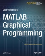
An algorithm for modulation of communications that generates 1024 random bits, performs modulation, adds complex Gaussian noise and graphically represents the result is represented in Figure 1-2. All in just lines of code in MATLAB.

MATLAB enables you to execute commands or groups of commands one at a time, with no compile or link, to achieve the optimal solution.

To quickly execute complex vector and matrix calculations, MATLAB uses libraries optimized for the processor. For many of its calculations, MATLAB generates instructions into machine code using JIT (Just-In-Time) technology. Thanks to this technology, which is available for most platforms, execution speeds are much faster than with traditional programming languages.

MATLAB includes development tools, which help efficiently implement algorithms. The following are some of them:

• MATLAB Editor – With editing functions and standard debugging offerings such as setting breakpoints and step by step simulations
• M-Lint Code Checker – Analyzes the code and recommends changes to improve the performance and maintenance (Figure 1-3)

  

  Figure 1-3.

• MATLAB Profiler – Records the time that it takes to execute each line of code
• Directory Reports – Scans all files in a directory and creates reports about the efficiency of the code, the differences between files, dependencies of the files and code coverage

You can also use the interactive tool GUIDE (Graphical User Interface Development Environment) to design and edit user interfaces. This tool allows you to include pick lists, drop-down menus, push buttons, radio buttons and sliders, as well as MATLAB diagrams and ActiveX controls. You can also create graphical user interfaces by means of programming using MATLAB functions. You can also expose figures or MATLAB algorithms on the web.

Figure 1-4 shows the analysis of wavelets in the tool user interface using GUIDE (above) and the interface (below) completed.

1.1.2 Data Access and Analysis

MATLAB supports the entire process of data analysis, from the acquisition of data from external devices and databases, pre-processing, visualization and numerical analysis, up to the production of results in presentation quality.

MATLAB provides interactive tools and command line operations for data analysis, which include: sections of data, scaling and averaging, interpolation, thresholding and smoothing, correlation, analysis of Fourier and filtering, search for one-dimensional peaks and zeros, basic statistics and curve fitting, matrix analysis, etc.

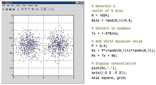
Figure 1-5 shows a diagram that shows a curve adjusted to atmospheric pressure differences averaged between Easter Island and Darwin in Australia.

In terms of access to data, MATLAB is an efficient platform for access to data files, other applications, databases and external devices. You can read data stored in most known formats, such as Microsoft Excel, ASCII text files or binary files of images, sound and video, and scientific archives such as HDF and HDF5 files. The binary files for low level I/O functions allow you to work with data files in any format. Additional features allow you to view web pages and XML data.

It is possible to call other applications and languages, such as C, C++, COM, DLLs, Java, Fortran, and Microsoft Excel objects and access FTP sites and web services. Using the Database Toolbox, you can access ODBC/JDBC databases.

1.1.3 Data Visualization

All graphics functions necessary to visualize scientific and engineering data are available in MATLAB. MATLAB includes features for representation of two-dimensional and three-dimensional diagrams, three-dimensional volume visualization, tools to create diagrams interactively and the possibility of exporting to the most popular graphic formats. It is possible to customize diagrams adding multi-axes, change the colors of the lines and markers, add annotations, LaTeX equations, legends and other plotting options.

Vectors functions represented by two-dimensional diagrams can be viewed to create:

• Diagrams of lines, area, bars and sectors
• Direction and velocity diagrams
• Histograms
• Polygons and surfaces
• Dispersion bubble diagrams
• Animations

Figure 1-6 shows linear plots of the results of several tests of emissions of a motor, with a curve fitted to the data.

MATLAB also provides functions for displaying two-dimensional arrays, three-dimensional scalar data and three-dimensional vector data. It is possible to use these functions to visualize and understand large amounts of multidimensional data that is usually complex. It is also possible to define the characteristics of the diagrams, such as the orientation angle of the camera, perspective, lighting effects, the location of the source of light and transparency. 3D diagramming features include:

• Surface, contour and mesh
• Diagrams of images
• Cone, pastel, flow and isosurface

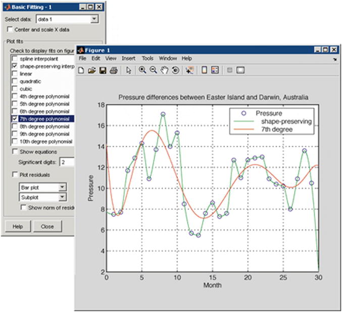
Figure 1-7 shows a three-dimensional diagram of an isosurface that reveals the GEODESIC domed structure of a fullerene carbon-60 molecule.

MATLAB includes interactive tools for design and graphics editing. From a MATLAB diagram, you can perform any of the following tasks:

• Drag and drop new sets of data in a figure
• Change the properties of any object in the figure
• Change the zoom, rotation, add a panoramic view, or change the camera angle and lighting
• Add data labels and annotations
• Draw shapes
• Generate a code M file that represents a figure for reuse with different data

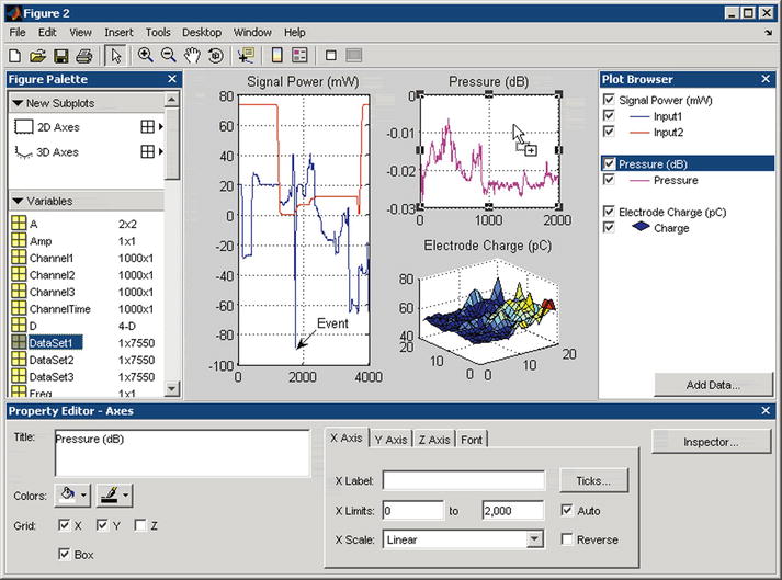
Figure 1-8 shows a collection of graphics, created interactively by dragging data sets onto the diagrams window, creating new subdiagrams, changing properties such as colors and fonts and adding annotations.

MATLAB is compatible with the common file formats of data and best-known graphics formats, such as GIF, JPEG, BMP, EPS, TIFF, PNG, HDF, AVI, and PCX. As a result, it is possible to export MATLAB diagrams to other applications, such as Microsoft Word and Microsoft PowerPoint, or desktop publishing software. Before exporting, you can create and apply style templates that contain designs, fonts, the definition of the thickness of lines, etc., necessary to comply with the specifications for publication.

1.1.4 Numeric Calculation

MATLAB contains mathematical, statistical, and engineering functions that support most of the operations to be carried out in these fields. These functions, developed by math experts, are the foundation of the MATLAB language. To cite some examples, MATLAB implements the following math and analysis functions for data in the following fields:

• Manipulation of matrices and linear algebra
• Polynomials and interpolation
• Differential and integral calculus
• Fourier analysis and filters
• Statistics and data analysis
• Optimization and numerical integration
• Ordinary differential equations (ODEs)
• Differential equations in partial derivatives (PDEs)
• Sparse matrix operations

1.1.5 Results Publication and Applications Distribution

In addition, MATLAB contains a number of functions to document and share work. You can integrate your MATLAB code with other languages and applications, and distribute their algorithms and MATLAB applications as autonomous programs or software modules.

MATLAB allows you to export the results in the form of diagrams or complete reports. You can export diagrams to all graphics formats to then import them into other packages such as Microsoft Word or Microsoft PowerPoint. Using MATLAB Editor, you can automatically publish your MATLAB code in HTML format, Word, LaTeX, etc.. Figure 1-9 shows  the M file (left) program published in HTML (right) using MATLAB Editor. The results, which are sent to the Command Window or diagrams, are captured and included in the document and the comments become titles and text in HTML.

It is possible to create more complex reports, such as mock executions and various tests of parameters, using MATLAB Report Generator (available separately).

In terms of the integration of the MATLAB code with other languages and applications, MATLAB provides functions to integrate code C and C++, Fortran code, COM objects, and Java code in your applications. You can call DLLs and Java classes and ActiveX controls. Using the MATLAB engine library, you can also call MATLAB from C, C++, or Fortran code.

For distribution of applications, you can create algorithms in MATLAB and distribute them to other users of MATLAB M file using the MATLAB Compiler (available separately). Algorithms can be distributed, either as standalone applications or as modules in software for users who do not have MATLAB. Additional products can be used to turn algorithms into a software module that can be called from COM or Microsoft Excel.

1.2 MATLAB Working Environment

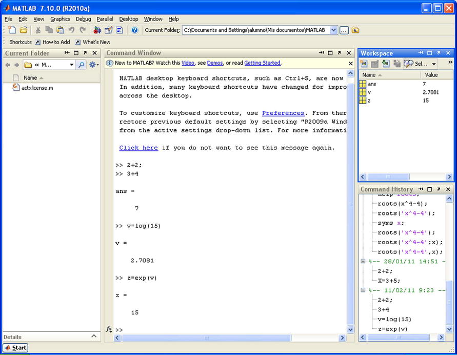
Figure 1-10 shows the screen used for entering the program, which is the primary MATLAB work environment.

The following table summarizes the components of the MATLAB environment.

Any input to run MATLAB is written to the right of the user input prompt “>>” which in turn, generates the response in the lines immediately below it. On completion, MATLAB displays the user input prompt again so that you can introduce more entries (Figure 1-13).

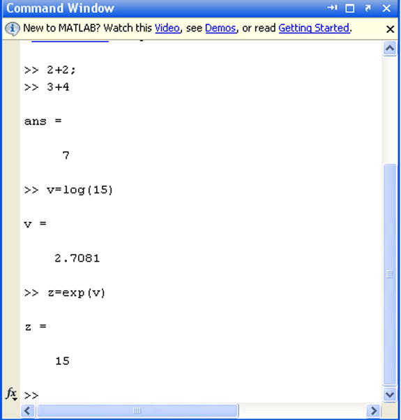
When an input (user input) is proposed to MATLAB in the Command Window that does not cite a variable to collect the result, MATLAB returns the response using the expression ans= as shown at the beginning of Figure 1-13. If at the start of our input to MATLAB, we define a variable to contain the results, we can then use that variable as the argument for subsequent entries. That is the case with variable v in Figure 1-13, which is subsequently used as input in an exponential function call.

To run an input entry, simply press Enter once you have finished. If at any point in the input we put a semicolon, the program runs calculations to that point and keeps them in memory (Workspace), but it does not display the result on the screen (see the first input in Figure 1-13). After you have hit Enter, MATLAB will respond and when it is done, the input prompt again appears “>> ” to indicate that you can enter a new command, function, etc.

Like the C programming language, MATLAB is sensitive to the difference between uppercase and lowercase letters; for example, Sin (x) is different from sin (x). The names of all MATLAB built-in functions begin with lowercase. There should be no spaces in the names of functions or in symbols of more than one letter. In other cases, spaces are ignored. They can be used to make input more readable. To save time you can provide input for multiple entries separated by commas on the same line of a command,, and pressing Enter at the end of the last entry will run each of the MATLAB responses separately (Figure 1-14). If you use a semicolon at the end of one of the entries of the line, its corresponding output is not displayed.

It is possible to enter descriptive comments in a command input line starting them with the “%” sign. When you run the input, MATLAB ignores the comment area and processes the rest.

>> L = log (123)

L =

   4.8122

To simplify the process of the introduction of scripts to be evaluated by the interpreter of MATLAB (via the Command Window), you can use the arrow computer keys to access the command history. For example, if you press the up arrow once, we recover the last entry submitted in MATLAB. If you press the key up twice, it recovers the penultimate entry submitted, and so on.

If you type a sequence of characters in the input area and then click the up arrow, MATLAB recovers the last entry that begins with the specified string.

Commands entered during a MATLAB session are temporarily stored in the buffer (Workspace) until you end the session with the program, at which time they can be permanently stored in a file or you lose them permanently.

Below is a summary of the keys that can be used in the area of input of MATLAB (command line), as well as its functions:

The command clc clears the Command Window, but it does not delete the variables of the work area (that content remains in memory).

1.3 Help in MATLAB

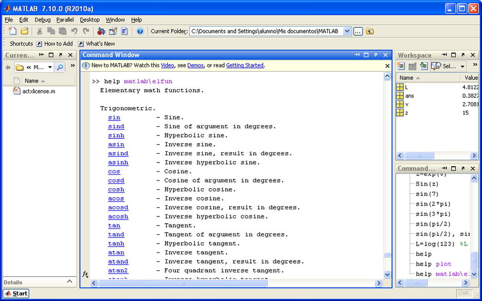
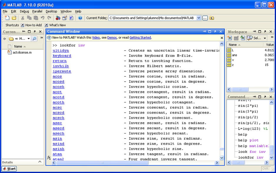
MATLAB help through the help button in the toolbar can be accessed here or through the Help menu bar option. In addition, support can also be obtained through commands implemented as MATLAB objects. The command help provides general help on all commands in MATLAB (Figure 1-15). By clicking on any of them, you get your particular help. For example, if you click on the hyperlink graph2d, you get support for graphics in two dimensions (Figure 1-16).

You can ask for help on a specific command (Figure 1-17) or on any subject content (Figure 1-18) using the command help command or help topic.

The command string lookfor allows you to find all those functions or commands of MATLAB that refer to your sequence or contain it. This command is very useful, to view all commands that contain the sequence. For example, if we seek help for all commands that contain the sequence investor, can use the command lookfor investor (Figure 1-19).

1.4 Numerical Calculations with MATLAB

You can use MATLAB as a powerful numerical calculator. Most calculators handle numbers only with a preset degree of precision, however MATLAB performs exact calculations with necessary precision. In addition, unlike calculators, we can perform operations not only with individual numbers, but also with objects such as arrays.

Most of the themes of the classical numerical calculations, are treated in this software. It supports matrix calculations, statistics, interpolation, fit by least squares, numerical integration, minimization of functions, linear programming, numerical algebraic and resolution of differential equations and a long list of processes of numerical analysis that we’ll see later in this book.

Here are some examples of numerical calculations with MATLAB. (As we all know, for results it is necessary to press Enter once you have written the corresponding expressions next to the prompt “>>”)

We can simply calculate 4 + 3 and get as a result 7. To do this, just type 4 + 3, and then Enter.

>> 4 + 3

Ans =

7

Also we can get the value of 3 to the 100^th power, without having previously set precision. For this purpose press 3 ^ 100.

>> 3 ^ 100

Ans =

5. 1538e + 047

You can use the command “format long e” to return the result of the operation with 16 digits before the exponent (scientific notation).

>> format long e

>> 3^100

ans =

5.153775207320115e+047

we also can work with complex numbers. We will get the result of the operation (2 + 3i) raised to the 10^th power, by typing the expression (2 + 3i) ^ 10.

>> (2 + 3i) ^ 10

Ans =

-1 415249999999998e + 005 - 1. 456680000000000e + 005i

(5) The previous result is also available in short format, using the “format short” command.

>> format short
>> (2 + 3i)^10

ans =

-1.4152e+005- 1.4567e+005i

Also we can calculate the value of the Bessel function found in section 11.5. To do this type Besselj (0,11.5).

>> besselj(0,11.5)

ans =

   -0.0677

1.5 Symbolic Calculations with MATLAB

MATLAB handles symbolic mathematical computation using the Symbolic Math Toolbox, manipulating formulae and algebraic expressions easily and quickly and can perform most operations with them. You can expand, factor and simplify polynomials, rational and trigonometric expressions, you can find algebraic solutions of polynomial equations and systems of equations, can evaluate derivatives and integrals symbolically, and find function solutions for differential equations, you can manipulate powers, limits and many other facets of algebraic mathematical series.

To perform this task, MATLAB requires all the variables (or algebraic expressions) to be written between single quotes to distinguish them from numerical solutions. When MATLAB receives a variable or expression in quotes, it is considered symbolic.

Here are some examples of symbolic computation with MATLAB.

1. You can raise the following algebraic expression to the third power: (x + 1) (x+2) - (x+2) ^ 2. This is done by typing the following expression: expand (‘((x + 1) (x+2) - (x+2) ^ 2) ^ 3’). The result will be another algebraic expression:

   >> syms x; expand (((x + 1) *(x + 2)-(x + 2) ^ 2) ^ 3)
   
   Ans =
   
   -x ^ 3-6 * x ^ 2-12 * x-8

   Note that syms x is used to declare x for symbolic computations.

   You can then factor the result of the calculation in the example above by typing: factor (‘((x + 1) *(x + 2)-(x + 2) ^ 2) ^ 3’)

   >> syms x; factor(((x + 1)*(x + 2)-(x + 2)^2)^3)
   
   ans =
   
   -(x+2)^3

2. You can resolve the indefinite integral of the function (x ^ 2) Sine (x) ^ 2 by typing: int (‘x ^ 2 * sin (x) ^ 2’, ‘x’)

   >> int('x^2*sin(x)^2', 'x')
   
   ans =
   
   x ^ 2 * (-1/2 * cos (x) * sin (x) + 1/2 * x)-1/2 * x * cos (x) ^ 2 + 1/4 * cos (x) * sin (x) + 1/4 * 1/x-3 * x ^ 3

   You can simplify the previous result:

   >> syms x; simplify(int(x^2*sin(x)^2, x))
   
   ans =
   
   sin(2*x)/8 - (x*cos(2*x))/4 - (x^2*sin(2*x))/4 + x^3/6

   You can express the previous result with more elegant mathematical notation:

   >> syms x; pretty(simplify(int(x^2*sin(x)^2, x)))
   
                              2             3
     sin(2 x)   x cos(2 x)   x  sin(2 x)   x
     -------- - ---------- - ----------- + --
        8           4             4        6

3. We can solve the equation 3ax - 7 x ^ 2 + x ^ 3 = 0 (where a, is a parameter):

   >> solve('3*a*x-7*x^2 + x^3 = 0', 'x')
   
   ans =
   
   [                          0]
   [7/2 + 1/2 *(49-12*a) ^(1/2)]
   [7/2 - 1/2 *(49-12*a) ^(1/2)]

4. We can find the five solutions of the equation x ^ 5 + 2 x + 1 = 0:

   ans =
   
                                            -0.48638903593454300001655725369801
      0.94506808682313338631496614476119 + 0.85451751443904587692179191887616*i
      0.94506808682313338631496614476119 - 0.85451751443904587692179191887616*i
    - 0.70187356885586188630668751791218 - 0.87969719792982402287026727381769*i
    - 0.70187356885586188630668751791218 + 0.87969719792982402287026727381769*i

As mentioned before, MATLAB can be extended by utilizing other libraries to extend its functionality. In particular, MATLAB may use the libraries of the Maple V program, to work with symbolic math and can thus extend its field of action. In this way, you can use MATLAB to work on issues such as differential forms, Euclidean geometry, projective geometry, statistics, etc.

At the same time, you also can expand the topics of numerical calculation, using the libraries from MATLAB and libraries of Maple (combinatorics, optimization, theory of numbers, etc.)

1.6 Graphics with MATLAB

MATLAB produces graphs of two and three dimensions, as well as outlines and graphics of density. You can represent the graphics and list the data. MATLAB allows you to control colors, shading and other graphics features, also supports animated graphics. Graphics produced by MATLAB are portable to other programs.

Here are some examples of MATLAB graphics:

1. You can represent the function xSine (x) for x ranging between -π/4 and π/4 taking 300 equidistant points for the intervals. See Figure 1-20.

   >> x = linspace(-pi/4,pi/4,300);
   >> y = x.*sin(1./x);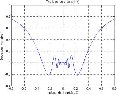
   >> plot(x,y)0

   

   Figure 1-20.

2. You can give the graph above the options frame and grille, as well create your own chart title and labels for axes. See Figure 1-21.

   >> x = linspace(-pi/4,pi/4,300);
   >> y = x.*sin(1./x);
   >> plot(x,y);
   >> grid;
   >> xlabel('Independent variable X'),
   >> ylabel ('Independent variable Y'),
   >> title ('The function y=xsin(1/x)')

   

   Figure 1-21.

3. You can generate a graph of the surface for the function z = Sin (sqrt(x^2+y^2)) /sqrt(x^2+y^2), making the variables (also axes) x and y span the range of -7.5 to +7.5 in 0.5 increments. See Figure 1-22.

   >> x =-7.5:.5:7.5;
   >> y = x;
   >> [X, Y] = meshgrid(x,y);
   >> Z = sin(sqrt(X.^2+Y.^2))./sqrt(X.^2+Y.^2);
   >> surf (X, Y, Z)

   

   Figure 1-22.

   These 3D graphics allow you to get an idea of the figures in space, and are very helpful in visually identifying intersections between different bodies, generation of developments of all kinds and volumes of revolution.

4. You can generate a three dimensional graphic corresponding to the Helix in parametric coordinates: x = Sin (t), y = Cos(t), z = t. See Figure 1-23.

   >> t = 0:pi/50:10*pi;
   >> plot3(sin(t),cos(t),t)

   

   Figure 1-23.

5. We can represent a planar curve given by its polar coordinates r = Cos (2t) * Sine (2t) for t varying between 0 and π, taking equally spaced points in one-hundredths of the considered range. See Figure 1-24.

   >> t = 0:.1:2 * pi;
   >> r = sin(2*t).* cos(2*t);
   >> polar(t,r)

   

   Figure 1-24.

6. We can also make a graph of a function considered as symbolic, using the command “ezplot”. See Figure 1-25.

   >> y ='x ^ 3 /(x^2-1)';
   >> ezplot(y,[-5,5])

   

   Figure 1-25.

In the corresponding chapter of graphics we will extend these concepts.

1.7 MATLAB and Programming

Programs usually consist of a series of instructions in which values are calculated, are assigned a name or value and are reused in further calculations.

As in programming languages like C or Fortran, in MATLAB you can write programs with loops, control flow and conditionals. In MATLAB you can write procedural programs, i.e., to define a sequence of standard steps to run. As in C or Pascal, a Do, For, or While may be used for repetitive calculations to be performed. The language of MATLAB also includes conditional constructs such as If Then Else. MATLAB also supports different logic functions, such as And, Or, Not and Xor.

MATLAB supports procedural programming (iterative, recursive, loops...), functional programming and object-oriented programming. Here are two simple examples of programs. For our purposes, he first generates the order n Hilbert matrix (which can also be gotten by using hilb(n), and the second calculates the Fibonacci numbers for values less than 1000.

% Generating the order n Hilbert matrix
t = '1/(i+j-1)';
for i = 1:n
for j = 1:n
a(i,j) = eval(t);
end
end

% Calculating Fibonacci numbers
f = [1 2 3]
i = 1;
while f(i) + f(i-1) < 1000
f(i+2) = f(i) + f(i+1);
i = i+1;
end