![]()
Display Volumes and Specialized Graphics
4.1 Volumes Visualization
MATLAB has a group of commands that allow you to represent different types of volumes. The following is the syntax of the most important.
coneplot(X, Y, Z, U, V, W, Cx, Cy, Cz) coneplot(U, V, W, Cx, Cy, Cz) coneplot(…,s) coneplot(…,color) coneplot(…,'quiver') coneplot(…,'method') coneplot(X, Y, Z, U, V, W, 'nointerp') h = coneplot(…) | Vector graphics cones in 3-D vector fields. (X, Y, Z) define the coordinates of the vector field. (U, V, W) define the vector field. (Cx, Cy, Cz) define the location of the cones in the vector field. In addition they may include arguments such as color, method of interpolation, etc. |
contourslice(X, Y, Z, V, Sx, Sy, Sz) contourslice(X, Y, Z, V, Xi, Yi, Zi) contourslice(V, Sx, Sy, Sz), contourslice (V, Xi, Yi, Zi) contourslice(…,n) contourslice(…, cvals) contourslice(…, [cv cv]) contourslice(…,'method') h = contourslice (…) | Draws outlines in planar sections of volumes according to the vectors (Sx, Sy, Sz). X, Y, Z define the coordinates for the volume V. Xi, Yi, Zi defined the surface along which the contour is drawn. You can use a method of interpolation and a number n of contour lines by plane. The value cv indicates a single-plane contour. |
[curlx, curly, curlz, cav] = curl(X,Y,Z,U,V,W) [curlx, curly, curlz, cav] = curl(U,V,W) [curlz, cav] = curl(X,Y,U,V) [curlz, cav] = curl(U,V) [curlx,curly,curlz] = curl(…), [curlx,curly] = curl(…) cav = curl(…) | This concerns the rotational curl and the angular velocity vector field cav. (X, Y, Z) arrays define the coordinates for the(U, V, W) vector field. In the case of curl(U,V,W) the conditions have to be [X Y Z] = meshgrid (1:n, 1:m, 1:p) with [m, n, p] = size(V) |
div = divergence(X,Y,Z,U,V,W) div = divergence(U,V,W) div = divergence(X,Y,U,V) div = divergence(U,V) | The divergence of a vector field |
interpstreamspeed(X,Y,Z,U,V,W,vertices) interpstreamspeed(U,V,W,vertices) interpstreamspeed(X,Y,Z,speed,vertices) interpstreamspeed(speed,vertices) interpstreamspeed(X,Y,U,V,vertices) interpstreamspeed(U,V,vertices) interpstreamspeed(X,Y,speed,vertices) interpstreamspeed(speed,vertices) interpstreamspeed(…,sf) vertsout = interpstreamspeed (…) | Interpolates streamline vertices based on the speed of the vector data. |
fvc = isocaps(X,Y,Z,V,isovalor) fvc = isocaps(V, isovalue) fvc = isocaps(…,'enclose') fvc = isocaps(…,'whichplane') [f, v, (c)] = isocaps(…) isocaps(…) | Concerns isosurfaces of volume V in the form value. X, Y, Z are the coordinates of the volume V. If it is not given, (X, Y, Z) is supposed to be [X, Y, Z] = meshgrid (1: n, 1:m, 1:p) with [m, n, p] = size (V). The value enclose may be ‘above’ or ‘below’, specifying whether the end-caps enclose data values above or below the value specified in isovalue. The values that can be provided for the whichplane parameter indicate the plane of drawing (all, xmin, xmax, ymin, ymax, zmin, and zmax). |
CN = isocolors(X,Y,Z,C,vertices) CN = isocolors(X,Y,Z,R,G,B,vertices) NC = isocolors (C, vertices) NC = isocolors (R, G, B, vertices) nc = isocolors(…,PatchHandle) isocolors(…,PatchHandle) | Computes the colors of the vertices of the isosurfaces using colors given as C or RGB values. PatchHandle vertices can be used. |
n = isonormals(X,Y,Z,V,vertices) n = isonormals(V, vertices) n = isonormals(V, p), n = isonormals(X,Y,Z,V,p) n = isonormals(…,'negate') isonormals(V, p), isonormals(X,Y,Z,V,p) | Computes normal vertices of isosurfaces. The negate option changes the direction of the normals and p is a vertex object identifier. If the n argument is not listed, the isonormals are drawn. |
FV = isosurface(X,Y,Z,V,isovalue) fv = isosurface(V, isovalue) FV = isosurface(X, Y, Z, V), FV = isosurface(X, Y, Z, V) fvc = isosurface(…,colors) fv = isosurface(…,'noshare') fv = isosurface(…,'verbose') [f, v] = isosurface(…) isosurface(…) | Extract data concerning the isosurfaces of volume V at the value specified in isovalue. The noshare argument indicates shared vertices will not be created and progress messages are printed to the command window as the function progresses through its computations. |
reducepatch(p,r) nfv = reducepatch(p,r) nfv = reducepatch(fv,r) reducepatch(…,'fast') reducepatch(…,'verbose') nfv = reducepatch(f,v,r) [NC, nv] = reducepatch (…) | It reduces the number of faces of the object identified by p with a factor of reduction r. The argument fast indicates that shared vertices are not computed, while NC and nv indicates that faces and vertices are returned. reducepatch(p) and NFV=reducepatch(FV) use a reduction factor of 0.5. |
[nx, ny, nz, nv] = reducevolume(X,Y,Z,V,[Rx,Ry,Rz]) [nx, ny, nz, nv] = reducevolume(V,[Rx,Ry,Rz]) nv = reducevolume(…) | Reduces the number of items in the data set of volume V whose coordinates are (X, Y, Z) arrays. Every Rx element is kept in the x direction, every Ry element is kept in the y direction, and every Rz element is kept in the z direction. For example, if Rx is 4, every fourth value in the x direction from the original dataset is retained. |
shrinkfaces(p,sf) nfv = shrinkfaces(p,sf) nfv = shrinkfaces(fv,sf) shrinkfaces(p), shrinkfaces(fv) nfv = shrinkfaces(f,v,sf) [nf,nv] = shrinkfaces(…) | Collapses the size of the faces of the object identified by p according to a contraction sf factor. If fv and sf are passed, the faces and vertices in fv are used. |
W = smooth3(V) W = smooth3(V,'filter') W = smooth3(V,'filter',size) W = smooth3(V,'filter',size,sd) | Smooths data of volume V. Smoothing with Gaussian or box filters.You can use a scalar or triple for anti-aliasing (size) and a standard deviation (sd); this only applies when ‘gaussian’ filter mode is used. |
XY = stream2(x,y,u,v,startx,starty) XY = stream2(u,v,startx,starty) | Finds lines of the current 2D vector data (u, v) whose coordinates are defined by the arrays (x, y) |
XYZ = stream3(X,Y,Z,U,V,W,startx,starty,startz) XYZ = stream3(U,V,W,startx,starty,startz) | Finds lines of the current 3D data vector (u, v, w) whose coordinates are defined by the arrays (x, y, z) |
h = streamline(X,Y,Z,U,V,W,startx,starty,startz) h = streamline(U,V,W,startx,starty,startz) h = streamline(XYZ) h = streamline(X,Y,U,V,startx,starty) h = streamline(U,V,startx,starty) h = streamline(XY) | Draw lines of the current 2D or 3D data vector. (X, Y, Z) are the coordinates of (U, V, W) and (startx, starty, startz) indicate the starting positions of the lines. |
streamparticles(vertices) streamparticles(vertices, n) | Draws the vector of the data field particles and represents them by markers in 2D or 3D vertices. |
streamribbon(X,Y,Z,U,V,W,startx,starty,startz) streamribbon(U,V,W,startx,starty,startz) streamribbon(vertices,X,Y,Z,cav,speed) streamribbon(vertices,cav,speed) streamribbon(vertices,twistangle) streamribbon(…,width), h = streamribbon(…) | Draws tapes for vector volume data (U, V, W) whose coordinates are (X, Y, Z) arrays using(startx, starty, startz) to indicate the positions of the start of the tapes. |
streamslice(X,Y,Z,U,V,W,startx,starty,startz) streamslice(U,V,W,startx,starty,startz) streamslice(X,Y,U,V) streamslice(U,V) streamslice(…,density) streamslice(…,'arrowmode') streamslice(…,'method') h = streamslice(…) [vertices arrowvertices] = streamslice(…) | Draws stream lines well spaced with arrow keys for the vector volume data (U, V, W) whose coordinates are (X, Y, Z), arrays where (startx, starty, startz) indicate the start positions of the lines. Density is a positive number that modifies the spacing of lines, arrows mode can use the values arrows or noarrows to put or not at the ends in the arrows, and method indicates the type of interpolation (linear, cubic, or nearest). |
streamtube(X,Y,Z,U,V,W,startx,starty,startz) streamtube(U,V,W,startx,starty,startz) streamtube(vertices,X,Y,Z,divergence) streamtube(vertices, divergence) streamtube(vertices,width) streamtube(vertices) streamtube(…,[scale n]) h = streamtube(…) | Draws tubes from vector volume data (U, V, W) whose coordinates are (X, Y, Z) arrays; (startx, starty, startz) indicate the start positions of the tubes. If the parameters vertices and divergence are used, then it is expected that [X Y Z] of vertices are sized as meshgrid(1:n, 1:m, 1:p) where [M N P] = size(divergence); width indicates the width of the tubes (which may be affected by a scale parameter n) |
fvc = surf2patch(h) fvc = surf2patch(Z) fvc = surf2patch(Z,C) fvc = surf2patch(X,Y,Z) fvc = surf2patch(X, Y, Z, C) fvc = surf2patch(…,'triangles') [f,v,c] = surf2patch(…) | Converts a given surface returning faces, vertices and color structure into the patch formatted structure fvc. The object can be given even as a surface in its different forms. You can also create triangular faces using the triangles argument. |
[Nx, Ny, Nz, Nv] = subvolume(X,Y,Z,V,limits) [Nx, Ny, Nz, Nv] = subvolume(V,limits) Nv = subvolume (…) | Extracts a subset of the volume V (X, Y, Z) using the given limits (limits = [xmin, xmax, ymin, ymax, zmin, zmax]) |
lims = volumebounds(X,Y,Z,V) lims = volumebounds(X,Y,Z,U,V,W) lims = volumebounds(V) lims = volumebounds(U,V,W) | Gives coordinates and boundaries of colors for the volume V (U, V, W) whose coordinates are (X, Y, Z) arrays. |
v = flow, v = flow(n) or v = flow(x,y,z) | Generates fluid flow data that is useful in functions that present volume data. When the x, y, and z parameters are used, the speed profile is evaluated. |
A first example are vectors that depict speed using cones in a vector field (Figure 4-1) from the default MATLAB data set wind.mat using the code below:
>> load wind
xmin = min(x(:)); xmax = max(x(:)); ymin = min(y(:));
ymax = max(y (:)); zmin = min(z(:));
daspect([2 2 1])
xrange = linspace(xmin,xmax,8);
yrange = linspace(ymin,ymax,8);
zrange = 3:4:15;
[cx cy cz] = meshgrid(xrange, yrange, zrange);
hcones = coneplot(x,y,z,u,v,w,cx,cy,cz,5);
set(hcones,'FaceColor','red','EdgeColor','none')

We then create planes along the axes (Figure 4-2).
>> hold on
wind_speed = sqrt(u.^2 + v.^2 + w.^2);
hsurfaces = slice(x,y,z,wind_speed,[xmin,xmax],ymax,zmin);
set(hsurfaces,'FaceColor','interp','EdgeColor','none')
hold off
Finally we define an appropriate point of view (Figure 4-3).
>> axis tight; view(30,40); axis off
They are then drawn as contours in planar sections of volumes on the data set wind.mat with a suitable point of view (Figure 4-4).
>> [x y z v] = flow;
h = contourslice(x,y,z,v,[1:9],[],[0],linspace(-8,2,10));
axis([0,10,-3,3,-3,3]); daspect([1,1,1])
set(gcf,'Color',[.5,.5,.5],'Renderer','zbuffer')
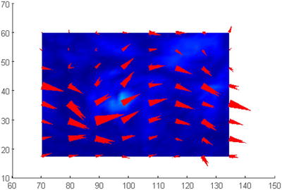
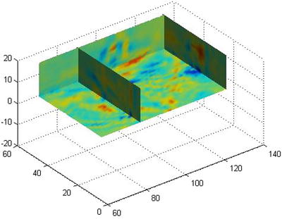
The following example shows the rotational vector field given by wind.mat using sections with colored drawings (Figure 4-5).
>> load wind
cav = curl(x,y,z,u,v,w);
slice(x,y,z,cav,[90 134],[59],[0]);
shading interp
daspect([1 1 1]); axis tight
colormap hot(16)
camlight

![]() Note camlight adds a light, just like a camera shoot. camlight with no parameters is the same as camlight right, which places the light above and to the right of the camera. Without this, the image would be much more yellow and orange and the vertical surface on the left would be much harder to perceive.
Note camlight adds a light, just like a camera shoot. camlight with no parameters is the same as camlight right, which places the light above and to the right of the camera. Without this, the image would be much more yellow and orange and the vertical surface on the left would be much harder to perceive.
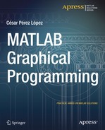
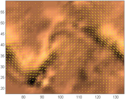
Below is code to show a representation on a plane (Figure 4-6).
>> load wind
k = 4;
x = x(:,:,k); y = y(:,:,k); u = u(:,:,k); v = v(:,:,k);
cav = curl(x,y,u,v);
pcolor(x,y,cav); shading interp
hold on;
quiver(x,y,u,v,'y')
hold off
colormap copper
The following example represents the divergence of the vector field given by wind.mat using sections with colored drawings (Figure 4-7).
>> load wind
div = divergence(x,y,z,u,v,w);
slice(x,y,z,div,[90 134],[59],[0]);
shading interp
daspect([1 1 1])
camlight
colormap jet
Below is an example concerning colors and normal for a given isosurface (Figure 4-8).
>> [x y z] = meshgrid(1:20,1:20,1:20);
data = sqrt(x.^2 + y.^2 + z.^2);
cdata = smooth3(rand(size(data)),'box',7);
p = patch(isosurface(x,y,z,data,10));
isonormals(x, y, z, data, p);
isocolors(x, y, z, cdata, p);
set(p,'FaceColor','interp','EdgeColor','none')
view(150,30); daspect([1 1 1]);axis tight
camlight; lighting phong;

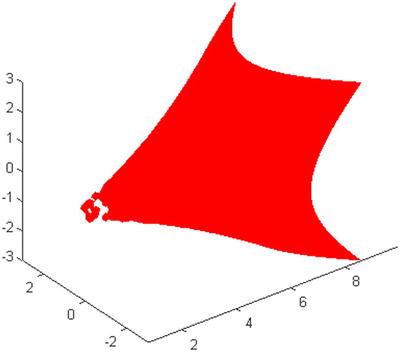
Subsequently represented is an isosurface (Figure 4-9) based on the wind.mat data set.
>> [x, y, z, v] = flow;
p = patch(isosurface(x,y,z,v,-3));
isonormals(x,y,z,v,p)
set(p,'FaceColor','blue','EdgeColor','none'),
daspect([1 1 1])
view(3); axis tight
In the following example (Figure 4-10), we reduce the faces of the anterior surface by 15% and show both images for comparison.
>> [x,y,z,v] = flow;
p = patch(isosurface(x,y,z,v,-3));
set(p,'facecolor','w','EdgeColor','b'),
daspect([1,1,1])
view(3)
figure;
h = axes;
p2 = copyobj(p,h);
reducepatch(p2,0.15)
daspect([1,1,1])
view(3)

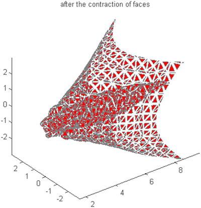
The following example reduces the volume of the previous isosurface (Figure 4-11) and then shrinks the size of their faces (Figure 4-12).
>> [x, y, z, v] = flow;
[x, y, z, v] = reducevolume(x,y,z,v,2);
FV = isosurface(x,y,z,v,-3);
p1 = patch(FV);
set(p1,'FaceColor','red','EdgeColor',[.5,.5,.5]);
daspect([1 1 1]); view(3); axis tight
title('Original')

>> figure
p2 = patch(shrinkfaces(FV,.3));
set(p2,'FaceColor','red','EdgeColor',[.5,.5,.5]);
daspect([1 1 1]); view (3); axis tight
title ('after the contraction of faces')

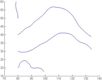
The following creates a chart with lines of two dimensional current (Figure 4-13) and then for three-dimensional (Figure 4-14).
>> load wind
[sx,sy] = meshgrid(80,20:10:50);
streamline(stream2(x(:,:,5),y(:,:,5),u(:,:,5),v(:,:,5),sx,sy));

>> load wind
[sx sy sz] = meshgrid(80,20:10:50,0:5:15);
streamline(stream3(x,y,z,u,v,w,sx,sy,sz))
view(3)

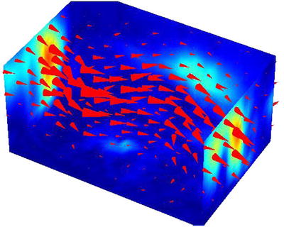
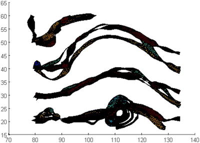
Below is a chart of tape (Figure 4-15) and one of tube (Figure 4-16).
>> load wind
[sx sy sz] = meshgrid(80,20:10:50,0:5:15);
daspect([1 1 1])
verts = stream3(x,y,z,u,v,w,sx,sy,sz);
CAV = curlx,y,z,u,v,w);
spd = sqrt(u.^2 + v.^2 + w.^2).*.1;
streamribbon(verts,x,y,z,CAV,spd)

>> load wind
[sx sy sz] = meshgrid(80,20:10:50,0:5:15);
daspect([1 1 1])
streamtube(x,y,z,u,v,w,sx,sy,sz);

4.2 Specialized Graphics
There are several types of specialized graphics that can be done with MATLAB (areas, boxes, graphics, three-dimensional sectors of Pareto, etc.) by using the commands that are presented in the following table.
area(Y) area(X, Y) area(…,ymin) | Makes the areas graph proportional to the values relative to the frequencies vector. When X is provided it represents the values of the X axis, at which each corresponding Y value will be plotted. Specifies the lower limit in the Y axis direction of the fill area |
box on, box off | Enable / disable boxes in axes for y in 3-D and 2-D graphics. |
comet(y) comet(x, y) comet(x, y, p) | Makes the comet graphic relative to the vector of frequencies y Performs the comet graphic relative to the frequencies vector Y whose elements are given by the vector X. Comet graph with body of length p * length |
ezcontour(f) ezcontour(f, domain) ezcontour(…,n) | Graphic of contour f(x,y) in [-2π, 2π] x [-2π, 2π]. So both the x and y parameters in the function are evaluated throughout the range of -2pi to +2pi. Graphic of contour f(x,y) in the given domain Graphic of contour f(x,y) in mesh n x n |
ezcontourf(f) ezcontourf(f, domain) ezcontourf(…,n) | Graphic of contour f(x,y) filling in [-2π, 2π] x [-2π, 2π]. Both the x and y parameters in the function are evaluated throughout the range of -2pi to +2pi. Graphic of contour f(x,y) filling in the given domain Graphic of contour f(x,y) stuffed in the mesh n x n |
ezmesh(f) ezmesh(f,domain) ezmesh(…,n) ezmesh(x, y, z) ezmesh(x, y, z, domain) ezmesh(…, 'circ') | Graph of f(x,y) mesh filling at [-2π, 2π] x [-2π, 2π]. Both the x and y parameters in the function are evaluated throughout the range of -2pi to +2pi. Graphic mesh of f(x,y) filling in the given domain Graph of f(x,y) mesh padding in the mesh nxn Graphic mesh for x = x(t,u), y = y(t,u), z = z(t,u) t,u Graphic mesh for x = x(t,u), y = y(t,u), z = z(t,u) t,u Graphic mesh on a disk centered in the domain |
ezmeshc(f) ezmeshc(f, domain) ezmeshc(…,n) ezmeshc(x, y, z) ezmeshc(x, y, z, domain) ezmeshc(…, 'circ') | Performs a combination of mesh and contour graphs. |
ezsurf(f) ezsurf(f, domain) ezsurf(…,n) ezsurf(x, y, z) ezsurf (x, y, z, domain) ezsurf(…, 'circ') | Makes a colored surface chart |
ezsurfc(f) ezsurfc(f, domain) ezsurfc(…,n) ezsurfc(x, y, z) ezsurfc (x, and z, domain) ezsurfc(…, 'circ') | Performs a combination of surface and contour graphs |
ezplot3(x, y, z) ezplot3(x, y,z, domain) ezplot3(…, 'animate') | Parametric curve 3D x = x (t), y = y(t), z = z (t) t Parametric curve 3D x = x (t), y = y(t), z = z (t) t Parametric curve for 3D animation |
ezpolar(f) ezpolar(f, [a, b]) | Graph the polar curve r = f (c) with c Graph the polar curve r = f (c) with c |
pareto(Y) pareto(X,Y) | Makes the graphic relative to the Pareto values vector of frequencies and Makes the graphic relative to the Pareto values vector whose elements are given by the vector X |
pie3(X) pie3(X, explode) | 3-D pie frequenciesvalues chart for X Detached three-dimensional pie chart |
plotmatrix(X, Y) | Scatter graph of the columns of X against Y |
quiver(U,V) quiver(X, Y, U, V) quiver(…, scale) quiver(…, LineSpec) quiver(…, LineSpec, 'filled') | Graph of velocity of the vectors with components (u, v) in the points (x, y). You can define a scale, specifications, line and fill. |
ribbon(y) ribbon(X, Y) ribbon(X, Y, width) | Graphic with three-dimensional tapes as columns. Graph X against the columns of Y. Specifies the width of the tape. |
stairs(Y) stairs(X, Y) stairs(…,LineSpec) | Stairstep graphic with elements of Y. Stairstep graphic with elements of Y corresponding with X. When the LineSpec parameter is used, colors can be controlled using ‘r’=red, and so on. |
scatter(X,Y,S,C) scatter(X,Y) scatter(X,Y,S) scatter(…, marker) scatter(…, 'filled') | Dispersion for the vector graph (X, Y) according to color C and the area of each marker S. You can also get the graphic filled (fill option) and use different types of markers. |
scatter3(X,Y,Z,S,C) scatter3(X,Y,Z) scatter3(X,Y,Z,S) scatter3(…,marker) scatter(…,'filled') | Graphic three-dimensional scatter (X, Y, Z) vectors according to the colors C and the area of each marker S. You can also get the graphic filled (fill option) and use different types of markers. |
TRI = delaunay(x,y) | Delaunay Triangulation. |
K = dsearch(x,y,TRI,xi,yi) | Delaunay Triangulation for the nearest point. |
IN = inpolygon(X,Y,xv,yv) | Detects points inside a polygonal region. |
polyarea(X, Y) | Area of the polygon specified by vectors X and Y. |
tsearch | Delaunay Triangulation. |
voronoi(x,y) voronoi(x, y, TRI) | Voronoi diagrams. |
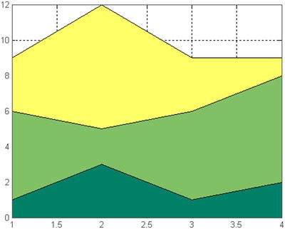
As a first example, we carry out a stacked area chart (see Figure 4-17).
>> Y = [1, 5, 3;
3, 2, 7;
1, 5, 3;
2, 6, 1];
area(Y)
grid on
colormap summer
We then create a two-dimensional Comet graph (Figure 4-18).
>> t = 0:.01:2 * pi;
x = cos(2*t) .* (cos (t) .^ 2);
y = sin(2*t) .* (sin (t) .^ 2);
comet(x,y);
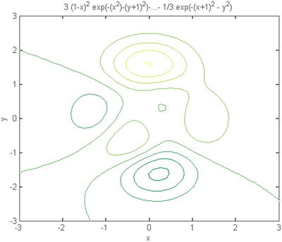
Then is the contour graphic (Figure 4-19) for the function:
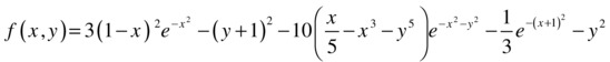
>> f = ['3 *(1-x)^2 * exp (-(x^2)-(y + 1)^2)','-10 *(x/5-x^3-y^5) * exp(-x^2-y^2)', '-1/3 * exp (-(x + 1)^2 - y^2)'];

>> ezcontour(f,[-3,3],49)
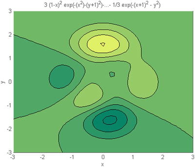
Then we fill the color in the previous contour (Figure 4-20).
>> ezcontourf(f,[-3,3],49)
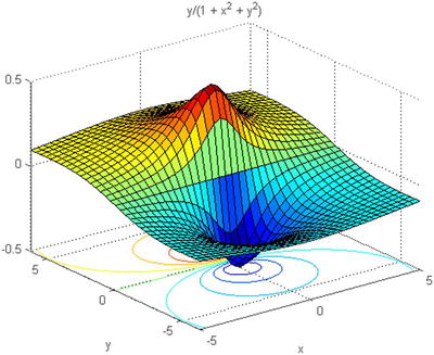
In the following example we do a mixed mesh-contour (Figure 4-21) for the function chart:
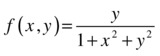
>> ezmeshc('y /(1 + x^2 + y^2)', [- 5, 5 - 2 * pi, 2 * pi])
colormap jet

Then the graphical surface and contour (Figure 4-22).
>> ezsurfc('y/(1 + x^2 + y^2)', [- 5, 5 - 2 * pi, 2 * pi], 35)
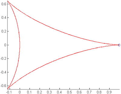
Then graph a curve in parametric space (Figure 4-23).
>> ezplot3('sin(t)','cos(t)','t’,[0,6*pi])

The following example builds a graph in three-dimensional sectors (Figure 4-24).
>> x = [1 3 0.5 2.5 2];
explode = [0 1 0 0 0];
pie3(x, explode)
colormap hsv

Then create a tape chart for surface peaks (Figure 4-25).
>> [x, y] = meshgrid(-3:.5:3,-3:.1:3);
z = peaks(x,y);
ribbon(y, z)
colormap hsv

The following example creates a stepped flat graph (Figure 4-26).
>> x = 0:.25:10;
stairs(x,sin(x))

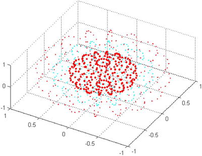
The following code creates a graph of a three-dimensional scatter plot (Figure 4-27).
>> [x, y, z] = sphere(16);
X = [x(:) *.5 x(:) *.75 x(:)];
Y = [y(:) *.5 y(:) *.75 y(:)];
Z = [z(:) *.5 z(:) *.75 z(:)];
S = repmat([1 0.75 0.5] * 10, prod(size(x)),1);
C = repmat([1 2 3],prod(size(x)),1);
scatter3(X(:),Y(:),Z(:),S(:),C(:),'filled'), view(-60,60)
Below is a polygonal area (Figure 4-28).
>> L = linspace(0,2.*pi,6); xv = cos(L)'; yv = sin(L)';
xv = [xv; xv(1)]; yv = [yv ; yv(1)];
A = polyarea(xv,yv);
plot(xv,yv); title(['Area = ' num2str(A)]); axis image

4.3 Special 3D Geometric Shapes
MATLAB provides commands to represent geometric shapes in three dimensions, such as cylinders, spheres, rods, sections, stems, waterfall, etc. The syntax of these commands is presented in the following table:
bar3(Y) | Bar graph relative to the frequencies values vector Y. If a matrix it gets multiple bar graphs for each row of Y. |
bar3(x,Y) | Bar graph relative to the values vector Y where x is a vector that defines the spaces in the x axis to locate bars. |
bar3(…,width) | Graph with given width of the bars. By default, the width is 0.8 and a width of 1 causes bars that touch. |
bar3(…,'style') | Graph with the given style bars. The styles are ‘detached’ (default style) ‘grouped’ (style with grouped vertical bars) and ‘stacked’ (stacked bars). |
bar3(…,color) | The bars are all of the specified color (r = red, g = green, b = blue, c = cyan, m = magenta y = yellow, k = black and w = white) |
comet3(z) comet3(x, y, z) comet3(x, y, z, p) | Graph relative to the Comet vector z Comet graph with parameters (x (t), y (t), z (t)) Comet graph of a kite with body of length p * length (y). |
[X, Y, Z] = cylinder [X, Y, Z] = cylinder(r) [X,Y, Z] = cylinder(r, n) cylinder(…) | It gives the coordinates of the unit cylinder. It gives the coordinates of the cylinder generated by the curve r. Gives the coordinates of the cylinder generated by the curve r with n points on the circumference that align the horizontal section with the Z axis (n = 20 by default). Graph previous cylinders. |
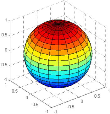
sphere | Graph the unit sphere using 20 x 20 faces. |
sphere(n) | Generates a sphere using n x n. |
[X, Y, Z] = sphere(n) | Gives the coordinates of the sphere in three arrays (n + 1) x (n + 1). |
slice(V,sx,sy,sz) slice(X,Y,Z,V,sx,sy,sz) slice(V,XI,YI,ZI) slice(X,Y,Z,V,XI,YI,ZI) slice(…,'method') | Draws slices along directions x, y and z in the volume V (array m x n x p) defined by the vectors (sx, sy, sz). Draws cuts defined by the vectors (sx, sy, sz) in the volume V, defined by the three-dimensional arrays (X, Y, Z). Draws cuts in volume V defined by (XI, YI, ZI) matrices that generate a surface. Draws cuts defined by (XI, YI, ZI) matrices that generate a surface in the volume V, defined by the three-dimensional arrays (X, Y, Z). Draws cuts according to the specified method of interpolation (linear, cubic and nearest). |
stem3(Z) stem3(X,Y,Z) stem3(…,'fill') stem3(…,S) | Draws the sequence Z as a graph of stems in the plane (x, y). Draws the sequence of values specified by X, Y and Z. Fill color in the circles at the tips of the stems. Makes stems utilize S specifications chart (color,…). |
waterfall(X,Y,Z) waterfall(Z) waterfall(…,C) | Draws a cascade graph according to the values of X, Y, Z. This means x = 1:size(Z,2) and y = 1:size(Z,1). Draws the cascade graph with colormap C. |
quiver3(X,Y,Z,U,V,W) | Draws the vectors of components (u, v, w) in the points (x, y, z). |
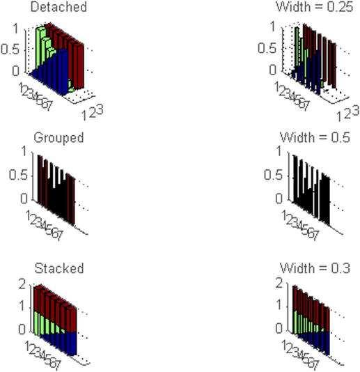
The first example presents a chart with various kinds of subgraphs (Figure 4-29) as three-dimensional bar charts.
>> Y = cool(7);
subplot(3,2,1)
bar3(Y,'detached')
title('Detached')

subplot(3,2,2)
bar3(Y,0.25,'detached')
title('Width = 0.25')

subplot(3,2,3)
bar3(Y,'grouped')
title('Grouped')

subplot(3,2,4)
bar3(Y,0.5,'grouped')
title('Width = 0.5')

subplot(3,2,5)
bar3(Y,'stacked')
title('Stacked')

subplot(3,2,6)
bar3(Y,0.3,'stacked')
title('Width = 0.3')
The following example creates a three-dimensional kite graph (Figure 4-30).
>> t = - 10 * pi: pi / 250:10 * pi;
comet3((cos(2*t) .^ 2) .* sin(t),(sin(2*t) .^ 2) .* cos(t),t);

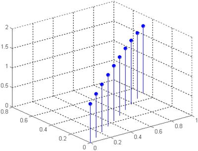
The following is the syntax that creates a graph of stems to display a function of two variables (Figure 4-31).
>> X = linspace(0,1,10);
Y = X / 2;
Z = sin (X) + cos (Y);
stem3(X,Y,Z,'fill')
Then draw the field unit with equal axes (Figure 4-32).
>> sphere
axis equal
Finally draw the cylinder unit within a square axis (Figure 4-33).
>> cylinder
axis square

4.4 Print, Export and Other Tasks with Graphics
The following table presents several commands of MATLAB which enable you to print graphics, select printer options and save graphics files.
orient orient landscape orient portrait orient tall | Situates the paper orientation for printing on your value by default. Situates the horizontal print orientation. Situated the vertical print orientation. Prints the entire page with portrait orientation. |
pagesetupdlg | Presents a dialog box to manage the position of the picture. |
print -device options file | Prints the chart using hardcopy. Print the graph to a file with given device options. |
printdlg printdlg(fig) | Prints the current figure. Creates a dialog for printing identified by fig. |
saveas(h,'file.ext') saveas(h,'file','format') | Save figure h in the graphic file file.ext. File guardian figure h in the file with the specified graphic format. |
According to extension, the graphic file formats are as follows:
Extension | Format |
|---|---|
AI | Adobe Illustrator' 88 |
BMP | Windows bitmap |
EMF | Enhanced metafile |
EPS | EPS Level 1 |
Fig | MATLAB figure |
jpg | JPEG image |
m | MATLAB M-file |
PBM | Portable bitmap |
PCX | Paintbrush 24-bit |
PGM | Portable Graymap |
PNG | Portable Network Graphics |
ppm | Portable Pixmap |
TIF | Image TIFF compressed image |