
![]()
Polynomials and Graphics Interpolation
6.1 Polynomial Expressions
The content of this chapter refers to work with polynomials and polynomial interpolation. We will study the commands that enable MATLAB to perform all operations with polynomials, working with their roots and polynomial interpolation.
MATLAB enables several commands for handling algebraic polynomial expressions. Let’s take a look at some of these commands:
- conv(a, b) gives the vector with the coefficients of the product of polynomials whose coefficients are elements of the vectors a and b.
- [q, r] = deconv(a, b) gives the vector q with the coefficients of the quotient of polynomials whose coefficients are elements of the vectors a and b, and the vector r, which is the polynomial remainder from division.
- poly2sym(a) is a Symbolic toolbox function that generates an object of the sym class creating the polynomial whose coefficients are those specified in the vector a.
- sym2poly(a) writes the vector of the specified polynomial coefficients (reverse operation to the previous one).
- roots(a) gives the roots of the polynomial whose coefficients are the vector a.
- poly(v) gives the polynomial whose roots are the components of the vector v.
- poly(A) gives the characteristic polynomial matrix A.
- polyder(a) gives the vector a whose coefficients are the first derivative of the polynomial.
- polyder(a, b) gives the vector whose coefficients are the derivative of the polynomial product of a and b.
- [q, d] = polyder(a, b) gives the coefficients of the numerator and denominator of the derivative of the polynomial quotient a/b.
- polyval(p, x, S) evaluates the polynomial p in x with standard deviation of the error equal to S.
- polyvalm(p, X) evaluates the polynomial p in matrix X.
- [r, p, k] = residue(a, b) gives the column vectors r, p and k such that:
- b(s)/a(s)=r1/(s-p1)+r2/(s-p2)+…+rn/(s-pn) +k(s)
- [b, a] = residue(r, p, k) performs the reverse of the previous operation.
Then let’s look at some examples of these newly defined commands:
Let’s decompose the fraction (-x ^ 2 + 2 x + 1) /(x^2-1)
>> [r,p,k]=residue([-1,2,1],[1,0,-1])

r =

1.0000
1.0000

p =

-1.0000
1.0000

k =

-1
So the decomposition will be:
(-x ^ 2 + 2 x + 1) /(x^2-1) = 1 /(-1+x) + 1 / (x + 1) - 1
The same result can be obtained in the following way:
>> pretty(sym(maple('convert((-x^2+2*x+1)/(x^2-1),parfrac,x)')))

       1       1
-1 + ---- + -----
      x     x + 1
Then we will evaluate the polynomial x ^ 4-6 * x ^ 3-x ^ 2 + 10 * x-11 about the point x = 5 and on the matrix of order 4.
>> polyval([1,-6,-1,10,-11],5)

ans =

-111

>> polyvalm([1,-6,-1,10,-11],ones(4))

ans =

-37 -26 -26 -26
-26 -37 -26 -26
-26 –26 -37 -26
-26 -26 –26 -37
Now let’s find the roots of the polynomial x ^ 3-x:
>> roots([1,0,-1,0])

Ans =

0
-1.0000
1.0000
Now solve the equation -x ^ 5 + 2 * x ^ 4 + x ^ 3 + x ^ 2 = 0:
>> roots([-1,2,1,1,0,0])

ans =

0
0
2.5468
-0.2734 + 0.5638i
-0.2734 - 0.5638i
EXERCISE 6-1
We consider the polynomial’s coefficients a = [2, -4, 5, 8, 0, 0, 1] and b = [-7, 15, 0, 12, 0]. Calculate the coefficients of the polynomials that are the product and quotient of a and b, also calculating the coefficients of the polynomials that are the derivatives of the products and the quotients of a and b.
>> a=[2,-4,5,8,0,0,1]; b=[-7,15,0,12,0];
>> conv(a,b)
ans =
-14 58 -95 43 72 60 89 15 0 12 0
>> [q,r]=deconv(a,b)
q =
-0.2857 -0.0408 -0.8017
r =
0 0 0 23.4548 0.4898 9.6210 1.0000
>> polyder(a)
ans =
12 -20 20 24 0 0
>> polyder(a,b)
ans =
-140 522 -760 301 432 300 356 45 0 12
>> [q, d] = polyder(a, b)
q =
-28 118 -120 251 -192 180 220 -45 0 -12
d =
49 -210 225 -168 360 0 144 0 0
The coefficient vectors can be transformed into the equivalent polynomials with the command poly2sym, resulting in polynomial form. Let’s see:
The product polynomial will be:
>> pretty(poly2sym(conv(a, b)))
10 9 8 7 6 5 4 3
-14 x + 58x - 95 x + 43 x + 72 x + 60 x + 89 x + 15 x + 12 x
The quotient polynomial is:
>> pretty(poly2sym(q))
9 8 7 6 5 4 3 2
- 28 x + 118 x - 120 x + 251 x - 192 x + 180 x + 220 x - 45 x - 12
The polynomial first derivative of a is :
>> pretty(poly2sym(polyder(a)))
5 4 3 2
12 x - 20 x + 20 x + 24 x
The polynomial first derivative of the product of a and b is:
>> pretty(poly2sym(polyder(a,b)))
9 8 7 6 5 4 3 2
-140 x + 522 x - 760 x + 301 x + 432 x + 300 x + 356 x + 45 x + 12
The polynomial quotient a/b will be q/d where q and d are:
>> [q,d]=polyder(a,b);
>> pretty(poly2sym(q))
9 8 7 6 5 4 3 2
-28 x + 118 x - 120 x + 251 x - 192 x + 180 x + 220 x - 45 x -12
>> pretty(poly2sym(d))
8 7 6 5 4 2
49 x - 210 x + 225 x - 168 x + 360 x + 144 x
EXERCISE 6-2
Find the characteristic polynomial of the matrix whose rows are vectors [2, -4, 5, 8], [0, 0, 0, 1], [-7, 15, 0.12] and [0, -1, -1, 0]. Also find the roots of this polynomial and check that the matrix satisfies the equation of your characteristic polynomial.
>> A=[2,-4,5,8;0,0,0,1;-7,15,0,12;0,-1,-1,0]
A =
2 -4 5 8
0 0 0 1
-7 15 0 12
0 -1 -1 0
>> p=poly(A)
p =
1.0000 -2.0000 48.0000 -67.0000 33.0000
>> pretty(poly2sym(p))
4 3 2
x - 2x + 48 x - 67 x + 33
To find the roots of the characteristic polynomial we use:
>> roots(p)
ans =
0.2836 + 6.8115i
0.2836 - 6.8115i
0.7164 + 0.4435i
0.7164 - 0.4435i
To verify that the matrix A satisfies the characteristic polynomial, we find the values in the polynomial Matrix A and observe that the result almost generates the null matrix.
>> polyvalm(p,A)
ans =
1.0e-012 *
-0.1990 0.1137 0.0266 0.5969
0.0093 -0.0711 -0.0071 0.0426
-0.0870 0.1137 -0.4192 -0.3979
0.0568 -0.1421 0.0013 -0.0497
EXERCISE 6-3
Expand the following operations in polynomial expressions.
3 2 2 3 3
a) (5 x y z - 4 x y z)
4 2 2 4
b) (x + y) (x + x y + y) (x - y)]
>> syms x y z
>> pretty(expand(simple(5*x^3*y^2*z-4*x*y^2*z^3)^3))
9 6 3 7 6 5 5 6 7 3 6 9
125 x y z - 300 x y z + 240 x y z - 64 x y z
>> pretty(expand((x+y) *(x^4+x^2*y^2+y^4) * (x-y)))
6 6
x -y
This shows that the polynomial presents difficulties of expansion when you use only the command expand.
EXERCISE 6-4
Factorize as much as possible the following polynomial expressions.
2 2 2 4 2 2
a. 4 x + y t + z - 4 x y t + 4 x z - 2 y t z
4 2 2 2 2 3 2
b. x - x y + 2 x y + x - 2 x - y
c. a m x + a m y - b m x - b m y + b n x - a n x - a n y + b n y
>> syms x y z b m n t
>> pretty(factor(4*x^2+y^2*t^2+z^4-4*x*y*t+4*x*z^2-2*y*t*z^2))
2 2
(2 x - y t + z)
>> pretty(factor(x^4-x^2*y^2+2*x*y^2+x^2-2*x^3-y^2))
2
(x - 1) (x - y) (x + y)
>> pretty(factor(a*m*x+a*m*y-b*m*x-b*m*y+b*n*x-a*n*x-a*n*y+b*n*y))
(x + y) (m - n) (a - b)
In general, in polynomial expressions, the command expand performs operations and simplifies the result, and the command factor factors the most.
>> pretty(expand((x-1)^2*(x-y)*(x+y)))
4 3 2 2 2 2 2
x - 2 x - x y + x + 2 x y - y
6.2 Interpolation and Polynomial Fit
MATLAB provides several commands for polynomial interpolation and adjustment curves that we will study below:
- polyfit(x, y, n) gives the vector of coefficients of the polynomial in x, p(x) of degree n that best fits the data (xi, yi) in the least squares sense (p(xi) = yi).
- Yí = interp1(X,Y,Xi, 'method') gives the vector Yi such that (Xi, Yi) is the total set of points found by interpolation between the given points (X, Y). The option method can take the value linear, spline, or cubic, depending on whether the interpolation is linear (default option), staggered or cubic (Xi points uniformly separated). This is for interpolation in one dimension.
- Zi = interp2(X,Y,Z,Xi,Yi, 'method') gives Zi where (Xi, Yi, Zi) is the total set of points found by interpolation between the given points (X, Y, Z). The option method can take the value linear or cubic, depending on whether the interpolation is linear (option by default) or cubic (Xi points uniformly separated). This is for two-dimensional interpolation.
- Zi = griddata(X,Y,Z,Xi,Yi) gives the vector Zi that determines the interpolation points (Xi, Yi, Zi) between the given points (X, Y, Z). A method of inverse distance is used to interpolate.
- Y = interpft(X,n) gives the vector Y uses the values of the periodic function X sampled at n equally spaced points. The original vector x is transformed to the domain of frequencies of a Fourier transform using the Fast Fourier transform (FFT algorithm). Valid for n ≥ length (X).
- maple('interp([exprx1,…,exprxn+1], [expry1,…,expryn+1],variable)') gives a polynomial in the specified variable of degree at least n that represents the interpoltion polynomial for points from [exprx1, expry1] to [exprxexpryn + 1n + 1]. The coordinates of the points all have to be different.
- maple('Interp([exprx1,…,exprxn+1], [expry1,…,expryn+1], variable)') in inert mode, is a polynomial in the specified variable of degree at least n that represents the interpolation polynomial for points from [exprx1, expry1] to [exprx n + 1 expryn + 1]. The coordinates of the points all have to be different.
- maple('Interp([exprx1,…,exprxn+1], [expry1,…,expryn+1], variable) mod n') in inert mode Module-n, is a polynomial in the specified variable of degree at least n that represents the interpolation polynomial for points from [exprx1, expry1] to [exprx n + 1 expryn + 1]. The coordinates of the points all have to be different.
- maple('readlib (thiele): thiele([exprx1,…,exprxn],[expry1,…,expryn],variable)') finds an expression in the given variable that represents the entire function resulting in the Thiele interpolation points (exprxi, expryi) for i = 1… n.
EXERCISE 6-5
Calculate the second degree interpolation polynomial passing through the points (-1,4), (0,2), and (1,6) in the least squares sense.
>> x=[-1,0,1];y=[4,2,6];p=poly2sym(polyfit(x,y,2))
p =
3 * x ^ 2 + x + 2
EXERCISE 6-6
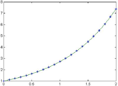
Represent 200 points of cubic interpolation between the points (x, y) given by the values that the function takes exponential e ^ x using 20x values equally spaced between 0 and 2. Also represent the difference between the function e ^ x and its approximation by interpolation. Use cubic interpolation.
First, we define the 20 given points (x, y), equally spaced between 0 and 2:
>> x = 0:0.1:2;
>> y = exp(x);
Now we find 200 points (xi, yi) for cubic interpolation, equally spaced between 0 and 2, and they are represented on a graph, together with the 20 points (x, y) using asterisks. See Figure 6-1:
>> xi = 0:0.01:2;
>> yi = interp1(x,y,xi,'cubic'),
>> plot(x,y,'*',xi,yi)
It now represents the difference between the exact values of the graph of y = e ^ x in 200 interpolation points and its own points (xi, yi). So you have a graphic idea of the error committed by using interpolation points instead of the exact points. The error would be zero if the graph was reduced to the x axis. See Figure 6-2:
>> zi=(exp(xi));
>> di=yi-zi ;
>> plot(xi,di)

EXERCISE 6-7
Get 25 points of approach by interpolation of the parametric function X = Cos(t), Y = Sin (t), Z = Tan(t) for values of t between 0 and π/6, on the set of points defined for values of t in the range 0 ≤ t ≤ 6.
First, we define the 25 given points (x, y, z), equally spaced between 0 and π / 6.
>> t = 0: pi/150: pi/6;
>> x = cos(t); y = sin(t); z = tan(t);
Now find the 25 points of interpolation (xi, yi, zi), for values of the parameter t equally spaced between 0 and π /6.
>> xi = cos(t); yi = sin(t);
>> zi = griddata(x,y,z,xi,yi);
>> points = [xi; yi; zi]’
points =
1.0000 0 0.0000
0.9998 0.0209 0.0161
0.9991 0.0419 0.0367
0.9980 0.0628 0.0598
0.9965 0.0837 0.0836
0.9945 0.1045 0.1057
0.9921 0.1253 0.1269
0.9893 0.1461 0.1480
0.9860 0.1668 0.1692
0.9823 0.1874 0.1907
0.9781 0.2079 0.2124
0.9736 0.2284 0.2344
0.9686 0.2487 0.2567
0.9632 0.2689 0.2792
0.9573 0.2890 0.3019
0.9511 0.3090 0.3249
0.9444 0.3289 0.3483
0.9373 0.3486 0.3719
0.9298 0.3681 0.3959
0.9219 0.3875 0.4203
0.9135 0.4067 0.4452
0.9048 0.4258 0.4706
0.8957 0.4446 0.4969
0.8862 0.4633 0.5236
0.8763 0.4818 0.5505
0.8660 0.5000 0.5774
EXERCISE 6-8
Get 30 points (xi, yi) for the periodic function y = Sin x for values of x that are equally spaced, interpolating them between 20 values of (x, y) given by y = sin (x) for x values evenly spaced in the interval (0, 2π), and using the interpolation method based on the fast Fourier transform (FFT).
First, we define the 20 x values equally spaced between 0 and 2π.
>> x = 0:pi/10:2*pi;
Now find the 30-point interpolation (x, y).
>> y = interpft(sin(x), 30);
>> points = [y; asin(y)]’
points =
0.0000 0.0000
0.1878 0.1890
0.4499 0.4667
0.6070 0.6522
0.7614 0.8654
0.9042 1.1295
0.9618 1.2935
0.9963 1.4848
0.9913 1.4388
0.9106 1.1448
0.8090 0.9425
0.6678 0.7312
0.4744 0.4943
0.2813 0.2852
0.0672 0.0673
-0.1640 - 0.1647
-0.3636 - 0.3722
-0.5597 - 0.5940
-0.7367 - 0.8282
-0.8538 - 1.0233
-0.9511 - 1.2566
-1.0035 - 1.5708 - 0. 0837i
-0.9818 - 1.3799
-0.9446 - 1.2365
-0.8526 - 1.0210
-0.6902 - 0.7617
-0.5484 - 0.5805
-0.3478 - 0.3553
-0.0807 - 0.0808
0.0086 0.0086
EXERCISE 6-9
Find the polynomial of degree 3 which better adjusts the cloud of points for the pairs (i, i2) where 1 ≤ i ≤ 7, in the least squares sense. Find your value for x = 10 and graphically represent the adjustment curve.
>> x=[1:7];y=[1,4,9,16,25,36,49];p=poly2sym(polyfit(x,y,2))
p =
x^2 - (5188368643045181*x)/633825300114114700748351602688 + 1315941209318717/79228162514264337593543950336
Now calculate the numerical value of the polynomial p for x = 10.
>> subs(p,10)
ans =
100
We can also approach the coefficients of the polynomial p to 5 digits.
>> vpa(p,5)
ans =
x^2 - 0.0000000000000081858*x + 0.00000000000001661
Figure 6-3 represents the graph of adjustment:
>> ezplot(p,[-5,5])
