Overview

Throughout this Part of the book, we’ve introduced some of the most basic components in a recommender system. In this chapter, we’ll get hands on. Now, we’re going to design and implement a recommender system for images from Pinterest. This kind of chapter, which we call Putting It All Together chapters, are more hands on and show you how to work with data sets using open source tools. The material for this kind of chapter refers to code hosted on GitHub that you will need to download and play with in order to properly experience these chapters.

Since this is the first practical hands on chapter, here are some extra setup instructions for the developement environment. We developed this code on Windows running in a Windows Subsystem for Linux Ubuntu virtual machine. It should run fine on Linux machines, with more technical adaptation for MacOS and a lot more for Windows, in which case it would be better to run it in a WSL2 Ubuntu virtual machine. You can look at the setup for WSL here Installing WSL. We picked Ubuntu for the image. You will also need CUDA and CUDNN if you have an nVidia GPU and want to use it.

We will be using the Shop the Look Data from Kang et al’s paper Complete the Look: Scene-based Complementary Product Recommendation.

In this chapter we will show how to build a content based recommender. Recall that a content based recommender uses indirect, generalizable representations of the items you wish to represent. Imagine for instance you want to recommend a cake but you cannot use the name of a cake. Instead you might use descriptions of a cake or the ingredients of a cake as the content features. With the Shop The Look Data set we will try to match scenes, which are pictures of a person in a particular setting, with products that might go well with the scene. The training set contains pairs of scenes with single products and we want to use the content recommender to extend recommendations to the entire catalog of products and sort them in some kind of ranking order. The content recommender, because it uses indirect content features to make recommendations, can be used to recommended new products that haven’t been in the recommender system or to warm start a recommender system with manually curated data before users start using it and a feedback loop is established. In the case of the Shop The Look data set, we’ll focus on the visual appearance of the scene and the products.

We will generate content embeddings via a convolutional neural network architecture, and then train the embedding via a triplet loss and show how to create a content recommender system.

This chapter will cover the following topics:

• Revision Control Software

• Python build systems

• Random Item Recommender

• Obtaining the STL dataset Images

• JAX

• Convolutional neural network definition

• Input pipeline

• Training the model in Flax and Optax

• Generating Embeddings

• Generating content based recommendations in JAX

Revision Control Software

Revision Control Software is a software system that keeps track of code changes. Think of it as a database that tracks versions of code you have written with added functionality like showing the differences between each version of code and reversion to previous versions of code.

There are many kinds of revision control systems out there. We host the code for this book on GitHub

The revision control software we use is called Git. Code changes are done in batches of changes called a patch and each patch is uploaded to a source control repository like GitHub so that they can be cloned and worked on by many people at the same time.

The command you can use to clone the book code sample repository is

git clone [email protected]:BBischof/ESRecsys.git

For this chapter, please look in the directory ESRecys/pinterest for instructions on how to run the code in detail. This chapter will mostly be descriptions and pointers to the repository so that you’ll able to get a feel for these systems in practice.

Python build systems

Python packages are libraries that provide functionality beyond the standard Python libraries. These include machine learning packages such as Tensorflow and JAX but also more utilitarian packages like the absl flags library or MLops libraries like Weights and Biases.

These packages are usually hosted on The Python Package Index

Take a look at the file requirements.txt

absl-py==1.1.0
tensorflow==2.9.1
typed-ast==1.5.4
typing_extensions==4.2.0
jax==0.3.25
flax==0.5.2
optax==0.1.2
wandb==0.13.4

You can see that we have picked a small set of Python packages to install for our dependencies. The format is package name, two equal signs and then the version of the package.

There are other build systems that work with Python such as

• pip

• Bazel Python

• Anaconda

For this chapter we will use pip.

Before we install the packages however, you might want to read up on Python virtual environments first.

Python virtual environments are a way to keep track of Python package dependencies per project so that if different projects use different versions of the same package they won’t interfere with each other because each project has it’s own Python virtual environment to run in.

You can create and activate a Python virtual environment by typing the following into a Unix shell:

python -m venv pinterest_venv
source pinterest_venv/bin/activate

The first command creates a python virtual environment and the second one activates it. You will have to activate a virtual environment everytime you open a new shell so that Python knows what environment to work in.

After the virtual environment is created you can then install packages using pip into the virtual environment and it will not affect the system level packages.

You can do this by running the following command in the ESRecsys/pinterest directory.

pip install -r requirements.txt

This will install the specified packages and any sub-packages that they might depend upon into the virtual environment.

Random Item Recommender

The first program we will look at is a random item recommender.

FLAGS = flags.FLAGS
_INPUT_FILE = flags.DEFINE_string(
  "input_file", None, "Input cat json file.")
_OUTPUT_HTML = flags.DEFINE_string(
  "output_html", None, "The output html file.")
_NUM_ITEMS = flags.DEFINE_integer(
  "num_items", 10, "Numer of items to recommend.")

# Required flag.
flags.mark_flag_as_required("input_file")
flags.mark_flag_as_required("output_html")

def read_catalog(catalog: str) -> Dict[str, str]:
    """
      Reads in the product to category catalog.
    """
    with open(catalog, "r") as f:
        data = f.read()
    result = json.loads(data)
    return result

def dump_html(subset, output_html:str) -> None:
    """
      Dumps a subset of items.
    """
    with open(output_html, "w") as f:
        f.write("<HTML>
")
        f.write("""
        <TABLE><tr>
        <th>Key</th>
        <th>Category</th>
        <th>Image</th>
        </tr>""")
        for item in subset:
            key, category = item
            url = pin_util.key_to_url(key)
            img_url = "<img src="%s">" % url
            out = "<tr><td>%s</td><td>%s</td><td>%s</td></tr>
" %
            (key, category, img_url)
            f.write(out)
        f.write("</TABLE></HTML>")

def main(argv):
    """
      Main function.
    """
    del argv  # Unused.

    catalog = read_catalog(_INPUT_FILE.value)
    catalog = list(catalog.items())
    random.shuffle(catalog)
    dump_html(catalog[:_NUM_ITEMS.value], _OUTPUT_HTML.value)

Here we use the absl flags library to pass in arguments to the program such as the path to the json catalog file that contains the shop the look scene, and product pairs.

Flags can have different types like string and integer and you can mark them as required. If a required flag is not passed to the program the program will complain and stop running.

Flags can be accessed via their value method.

We load and parse the STL dataset using the Python library json and then we randomly shuffle the catalog and dump the top few results in html.

You can run the random item recommender by running the following command

python3 random_item_recommender.py
--input_file=STL-Dataset/fashion-cat.json --output_html=output.html

After completion you can open the output.html file with your web browser and see some random items from the catalog. A sample of this can be seen in Figure 5-1.

Figure 5-1. Random Item Recommender

The fashion-catalog.json contains descriptions of products and their Pinterest ID while fashion.json contains pairings of a scene with a recommended product.

Next, we’ll look at how we can recommend multiple new items for a single scene by training a machine learning model on scene-product pairings.

It is generally a good idea to create a random item recommender the first time you encounter a corpus just so you have an idea of what kind of items are in the corpus and you have a baseline to compare to.

Obtaining the STL Dataset Images

The first step in the process of creating a content based recommender is fetching the content. In this case the Shop the Look dataset’s content is mostly images with some metadata about the image like the type of product. We will just be using the image content for this chapter.

You can look at the code in fetch_images.py to see how this is done, by using the Python standard libary urllib to fetch the images. Be aware that doing too much fetching on someone else’s website might trigger their bot defences and cause them to blacklist your IP address so it might be a wise idea to rate limit fetches or find some other way to get the data.

We have downloaded thousands of image files and put them together into an archive as a Weights and Biases artifact. Since it’s already in this artifact, you don’t need to scrape them yourself but the code we’ve supplied will allow you to do so.

You can read up on artifacts here WandB artifacts.

Artifacts are a MLOps (Machine Learning Operations) concept that version and package together archives of data and tracks producers and consumers of the data.

You can download the image artifact by running

wandb artifact get building-recsys/recsys-pinterest/shop_the_look:latest

The images will then be in the local directory artifacts/shop_the_look:v1

Convolutional Neural Network Definition

Now that we have the images, the next step is figuring out how to represent the data. Images come in different sizes and are a complex type of content to analyze. We can use the raw pixels as the representation of our content but the drawback of that is tiny changes in pixel values can cause large differences in the distance between images. We do not want that. Rather, we want to somehow learn what is important in the images and ignore parts of the image, such as the background color, that might not be as important.

For this task we will use a kind of convolutional neural network to compute an embedding vector for the image. An embedding vector is a kind of feature vector for the image that is learnt from data and is of fixed size. The reason we use embedding vectors for our representation is because we want out database to be small and compact, easy to score over large numbers of images in the corpus and to be relevant to the task at hand, which is to match products to a given scene image.

The neural network architecture we use is a variant of Residual Networks or Resnet. Please refer to He et al’s paper for details about the achitecture and for references on convolutional neural networks. Briefly, a convolution layer applies a small filter of typically 3x3 size repeatedly over an image. This results a feature map of the same resolution as the input if the stride is (1, 1) (which means apply the filter with a 1 pixel step in the x direction and a 1 pixel step in the y direction) or quarter size if the stride is (2, 2). The residual skip connection is just a short cut from the previous input layer to the next, so in effect the non-linear part of the networks learns the residual from the linear skip part, hence the name residual network.

Additionally we use the BatchNorm layer, details of which can be found at BatchNorm Paper and the Swish Nonlinearity.

Once we specify the model, we also need to optimize it for the task.

Jax, Flax and Optax

This optimization should be pretty straightforward to do in any machine learning framework. Here we show how to do it easily with Jax, Flax and Optax. Jax is a lower level numpy like machine learning library and Flax is a higher level neural network library that provides functionality such as neural network modules and embedding layers. Optax is a library that does optimization that we will use to minimize our loss function.

If you are familiar with numpy, Jax is quite easy to pick up. Jax shares the same api as numpy but has the capability of running the resulting code on vector processors such as GPUs or TPUs by doing just in time compilation or jit. Jax Device Arrays and numpy arrays can be easily converted back and forth which makes it easy to develop for the GPU and yet easy to debug on the CPU.

These packages can be found at the following websites:

• Jax

• Flax

• Optax

In addition to learning how to represent the images we also need to specify how they are related to each other.

Since the embedding vectors are of fixed dimension the easiest similarity score is simply the dot product of the two vectors. See “Similarity from co-occurrence” other kinds of similarity measures. So given an image for a scene, we compute the scene embedding and do the same for the product to obtain a product embedding and take the dot product of the two to obtain a score for the closeness of fit of a scene $\overrightarrow{s}$ to a product $\overrightarrow{p}$.

We use CNNs, or Convolutional Neural Networks to obtain the embedding of an image.

We use separate CNNs for the scene and product however, because they come from different kinds of images. Scenes tend to be about the context of what to match products to and contain people and the setting, whereas products tend to be catalog images of shoes and bags with a blank background so we need different neural networks to determine what is important in the image.

Once we have the score, that alone is not sufficient though. We need to make sure that a good match of a scene and product, which we call the positive product, is higher scoring than a negative product. The positive product is a good match for the scene and the negative product is a not so good match for the scene. The positive product comes from the training data and the negative product comes from randomly sampling the catalog. A loss that can capture the relationship between a positive scene-product pair (A, B) and negative scene-product pair (A, C) is called Triplet loss. We go into some detail for defining the Triplet Loss.

Suppose we want the score for the positive scene-product pair to be one more than a negative scene-product pair. We then have the following inequality:

1 is just an arbitrary constant we use, called a margin, to make sure that the positive scene product score is larger than the negative scene product score.

Since the process of gradient descent minimizes some function, we then convert the above inequality into a loss function by moving all terms to one side.

As long as the quantity on the right side is larger than zero we want to minimize it, but if it is already less than zero we do not, so we enclode the quantity in a rectified linear unit, which is represented by the function max(0, x). We can thus write out our loss function as follows:

Since we usually minimize loss functions this ensures that as long as the score(scene, neg_product) is 1 more than score(scene, pos_product) the optimization procedure will try to minimize the score of the negative pair while increasing the score of the positive pair.

In the following sections we will cover the following modules in order so that they make sense as they follow the flow of data from reading to training to making recommendations:

• input__pipeline.py - how the data is read

• models.py - how the neural networks are specified

• train_shop_the_look.py - how the neural network is fit using optax

• make_embeddings.py - how to make a compact database of scene and products

• make_recommendations.py - how to use the compact database of embeddings to create a list of product recommendations per scene

Input Pipeline

Here is the code for input_pipeline.py

We use the machine learning library Tensorflow for it’s data pipline.

import tensorflow as tf

def normalize_image(img):
  img = tf.cast(img, dtype=tf.float32)
  img = (img / 255.0) - 0.5
  return img

def process_image(x):
  x = tf.io.read_file(x)
  x = tf.io.decode_jpeg(x, channels=3)
  x = tf.image.resize_with_crop_or_pad(x, 512, 512)
  x = normalize_image(x)
  return x

def process_image_with_id(id):
  image = process_image(id)
  return id, image

def process_triplet(x):
  x = (process_image(x[0]), process_image(x[1]), process_image(x[2]))
  return x

def create_dataset(
    triplet: Sequence[Tuple[str, str, str]]):
    """Creates a triplet dataset.
    Args:
      triplet: filenames of scene, positive product, negative product.
    """
    ds = tf.data.Dataset.from_tensor_slices(triplet)
    ds = ds.map(process_triplet)
    return ds

You can see that create_dataset takes in three filenames, that of a scene, then a positive match and a negative match. For the purposes of this example, the negative match is simply selected at random from the catalog. There are more sophisticated ways of picking the negative that we will cover in a later chapter. The image file names are processed by reading the file, then decoding the image, cropping it to a fixed size and then rescaling the data so that it becomes a floating point image centered around 0 and with small values between -1 and 1. The reason we do this is most neural networks are initialized with the assumption that the data they get is roughly normally distributed and so if you pass in too large a value it would be far far out of the norm of the expected input range.

Here is how to specify our CNN and STL model with Flax.

from flax import linen as nn
import jax.numpy as jnp

class CNN(nn.Module):
    """Simple CNN."""
    filters : Sequence[int]
    output_size : int

    @nn.compact
    def __call__(self, x, train: bool = True):
        for filter in self.filters:
            # Stride 2 downsamples 2x.
            residual = nn.Conv(filter, (3, 3), (2, 2))(x)
            x = nn.Conv(filter, (3, 3), (2, 2))(x)
            x = nn.BatchNorm(
              use_running_average=not train, use_bias=False)(x)
            x = nn.swish(x)
            x = nn.Conv(filter, (1, 1), (1, 1))(x)
            x = nn.BatchNorm(
              use_running_average=not train, use_bias=False)(x)
            x = nn.swish(x)
            x = nn.Conv(filter, (1, 1), (1, 1))(x)
            x = nn.BatchNorm(
              use_running_average=not train, use_bias=False)(x)
            x = x + residual
            # Average pool downsamples 2x.
            x = nn.avg_pool(x, (3, 3), strides=(2, 2), padding="SAME")
        x = jnp.mean(x, axis=(1, 2))
        x = nn.Dense(self.output_size, dtype=jnp.float32)(x)
        return x

class STLModel(nn.Module):
    """Shop the look model that takes in a scene
        and item and computes a score for them.
    """
    output_size : int

    def setup(self):
        default_filter = [16, 32, 64, 128]
        self.scene_cnn = CNN(
          filters=default_filter, output_size=self.output_size)
        self.product_cnn = CNN(
          filters=default_filter, output_size=self.output_size)

    def get_scene_embed(self, scene):
        return self.scene_cnn(scene, False)

    def get_product_embed(self, product):
        return self.product_cnn(product, False)

    def __call__(self, scene, pos_product, neg_product,
                 train: bool = True):
        scene_embed = self.scene_cnn(scene, train)

        pos_product_embed = self.product_cnn(pos_product, train)
        pos_score = scene_embed * pos_product_embed
        pos_score = jnp.sum(pos_score, axis=-1)

        neg_product_embed = self.product_cnn(neg_product, train)
        neg_score = scene_embed * neg_product_embed
        neg_score = jnp.sum(neg_score, axis=-1)

        return pos_score, neg_score, scene_embed,
          pos_product_embed, neg_product_embed

Here we use Flax’s neural network class Module. The annotation nn.compact is there so we do not have to specify a setup function for simple neural network architectures like this one and can simply specify the layers in the call function. The call function accepts two parameters, an image x and a boolean train that tells the module if we are calling it in training mode or not. The reason we need it is that the BatchNorm layers are updated only during training, but they are not updated when the network is fully learned.

If you look at the CNN specification code you can see how we set up the Residual Network. We can mix neural network functions like swish with Jax functions mean freely. Swish is a function that is a non-linear activation for the neural network that transforms the input in such a way as to weight some values of activation more than others.

The STL Model on the other hand has more complicated setup, so we have to specify the setup code where we create two different towers of CNN, one for the scene and another one for the product. A CNN tower is just a copy of the same architecture but has different weights for different image corpora. As mentioned earlier, the reason we have a different tower for each type of image is that they represent different things, for the scene the context to which we are matching products to, and a separate tower for the products. As a result, we add in two different methods for converting scene and product images into scene and product embeddings. The call is also different. It doesn’t have the annotation compact because we have more complicated setup. In the call function for the STL model we first compute the scene embed, then the positive product embed and then the positive score. After that, we do the same for the negative score. We then return the positive score, negative score and also all three embedding vectors. We return the embedding vectors as well as the scores because we want to ensure that the model generalizes to new, unseen data as in a held out validation set, so we want to make sure they are not too large. This concept of capping the size of the embedding vectors so they are not too large is called regularization.

Now let’s take a look at train_shop_the_look.py. We’ll break it down into separate function calls and discuss them one by one.

def generate_triplets(
    scene_product: Sequence[Tuple[str, str]],
    num_neg: int) -> Sequence[Tuple[str, str, str]]:
    """Generate positive and negative triplets."""
    count = len(scene_product)
    train = []
    test = []
    key = jax.random.PRNGKey(0)
    for i in range(count):
        scene, pos = scene_product[i]
        is_test = i % 10 == 0
        key, subkey = jax.random.split(key)
        neg_indices = jax.random.randint(subkey, [num_neg], 0, count - 1)
        for neg_idx in neg_indices:
            _, neg = scene_product[neg_idx]
            if is_test:
                test.append((scene, pos, neg))
            else:
                train.append((scene, pos, neg))
    return train, test

 def shuffle_array(key, x):
    """Deterministic string shuffle."""
    num = len(x)
    to_swap = jax.random.randint(key, [num], 0, num - 1)
    return [x[t] for t in to_swap]

The first fragment of the code reads in the scene-product json database and generates triplets of scene, postive product and negative products for the input pipeline. The interesting part to note here is how Jax handles random numbers. Jax’s philosophy is very functional in nature, meaning that functions are pure and have no side effects. Random number generators carry state, so in order to make Jax random number generators function you have to pass in the state to the random number generator. The mechanism for this is to have Pseudo Random Number Generator Keys, PNRGKey, as the object carrying state. We initialize one arbitrarily from the number zero. Whenever we wish to use the key though, we have to split the key into two using jax.random.split and use the one to generate the next random number and a subkey to perform the random action. In this case we use the subkey to select a random negative from the entire corpus of products for our negative. There are more complex ways to sample the negative that we will cover in later chapters but randomly selecting a negative is the simplest way to construct the triplet for triplet loss.

Similarly to how the negatives are selected we again use Jax’s random functionality to generate a list of indices to swap in order to shuffle the array for the training step. Random shuffling is important in stochastic gradient descent to break up any kind of structure in the training data to ensure that the gradients are stochastic. We use Jax’s random shuffling mechansism for better reproduceability so that experiments are more likely to be the same given the same initial data and settings.

def train_step(state, scene, pos_product,
               neg_product, regularization, batch_size):
    def loss_fn(params):
        result, new_model_state = state.apply_fn(
            params,
            scene, pos_product, neg_product, True,
            mutable=['batch_stats'])
        triplet_loss = jnp.sum(nn.relu(1.0 + result[1] - result[0]))
        def reg_fn(embed):
            return nn.relu(
              jnp.sqrt(jnp.sum(jnp.square(embed), axis=-1)) - 1.0)
        reg_loss = reg_fn(result[2]) +
                   reg_fn(result[3]) + reg_fn(result[4])
        reg_loss = jnp.sum(reg_loss)
        return (triplet_loss + regularization * reg_loss) / batch_size

    grad_fn = jax.value_and_grad(loss_fn)
    loss, grads = grad_fn(state.params)
    new_state = state.apply_gradients(grads=grads)
    return new_state, loss

def eval_step(state, scene, pos_product, neg_product):
    def loss_fn(params):
        result, new_model_state = state.apply_fn(
            state.params,
            scene, pos_product, neg_product, True,
            mutable=['batch_stats'])
        # Use a fixed margin for the eval.
        triplet_loss = jnp.sum(nn.relu(1.0 + result[1] - result[0]))
        return triplet_loss

The next pair of functions we will look at are how the train and eval steps are written. The train step takes the state of the model, which contains the parameters of the model as well as the gradient information which depends on the optimizer being used. It also takes in batches of scenes, positive products and negative products in order to construct the triplet loss. In addition to optimizing for the triplet loss we also want to minimize the size of the embeddings whenever they go outside the unit sphere. This is called regularization, so we add it to the triplet loss to obtain the final loss.

Flax, being written on top of Jax is also functional in philosophy, so the existing state is used to compute the gradient of the loss function, which when applied returns a new state variable. This ensures that the functions remain pure and what is mutable is the state variables.

This functional philosophy is what allows Jax to Just In Time compile or JIT functions so they run fast on CPU, GPU or TPU.

The eval step in comparison is rather simple, it just computes the triplet loss without the regularization loss as our evaluation metric. Again we will cover more sophisticated evaluation metrics in later chapters.

def main(argv):
    """Main function."""
    del argv  # Unused.
    config = {
        "learning_rate" : _LEARNING_RATE.value,
        "regularization" : _REGULARIZATION.value,
        "output_size" : _OUTPUT_SIZE.value
    }

    run = wandb.init(
        config=config,
        project="recsys-pinterest"
    )

    tf.config.set_visible_devices([], 'GPU')
    tf.compat.v1.enable_eager_execution()
    logging.info("Image dir %s, input file %s",
      _IMAGE_DIRECTORY.value, _INPUT_FILE.value)
    scene_product = pin_util.get_valid_scene_product(
      _IMAGE_DIRECTORY.value, _INPUT_FILE.value)
    logging.info("Found %d valid scene product pairs." % len(scene_product))

    train, test = generate_triplets(scene_product, _NUM_NEG.value)
    num_train = len(train)
    num_test = len(test)
    logging.info("Train triplets %d", num_train)
    logging.info("Test triplets %d", num_test)

     # Random shuffle the train.
    key = jax.random.PRNGKey(0)
    train = shuffle_array(key, train)
    test = shuffle_array(key, test)
    train = np.array(train)
    test = np.array(test)

    train_ds = input_pipeline.create_dataset(train).repeat()
    train_ds = train_ds.batch(_BATCH_SIZE.value).prefetch(
      tf.data.AUTOTUNE)

    test_ds = input_pipeline.create_dataset(test).repeat()
    test_ds = test_ds.batch(_BATCH_SIZE.value)

    stl = models.STLModel(output_size=wandb.config.output_size)
    train_it = train_ds.as_numpy_iterator()
    test_it = test_ds.as_numpy_iterator()
    x = next(train_it)
    key, subkey = jax.random.split(key)
    params = stl.init(subkey, x[0], x[1], x[2])
    tx = optax.adam(learning_rate=wandb.config.learning_rate)
    state = train_state.TrainState.create(
        apply_fn=stl.apply, params=params, tx=tx)
    if _RESTORE_CHECKPOINT.value:
        state = checkpoints.restore_checkpoint(_WORKDIR.value, state)

    train_step_fn = jax.jit(train_step)
    eval_step_fn = jax.jit(eval_step)

    losses = []
    init_step = state.step
    logging.info("Starting at step %d", init_step)
    regularization = wandb.config.regularization
    batch_size = _BATCH_SIZE.value
    eval_steps = int(num_test / batch_size)
    for i in range(init_step, _MAX_STEPS.value + 1):
        batch = next(train_it)
        scene = batch[0]
        pos_product = batch[1]
        neg_product = batch[2]

        state, loss = train_step_fn(
            state, scene, pos_product, neg_product,
            regularization, batch_size)
        losses.append(loss)
        if i % _CHECKPOINT_EVERY_STEPS.value == 0 and i > 0:
            logging.info("Saving checkpoint")
            checkpoints.save_checkpoint(
              _WORKDIR.value, state, state.step, keep=3)
        metrics = {
            "step" : state.step
        }
        if i % _EVAL_EVERY_STEPS.value == 0 and i > 0:
            eval_loss = []
            for j in range(eval_steps):
                ebatch = next(test_it)
                escene = ebatch[0]
                epos_product = ebatch[1]
                eneg_product = ebatch[2]
                loss = eval_step_fn(
                  state, escene, epos_product, eneg_product)
                eval_loss.append(loss)
            eval_loss = jnp.mean(jnp.array(eval_loss)) / batch_size
            metrics.update({"eval_loss" : eval_loss})
        if i % _LOG_EVERY_STEPS.value == 0 and i > 0:
            mean_loss = jnp.mean(jnp.array(losses))
            losses = []
            metrics.update({"train_loss" : mean_loss})
            wandb.log(metrics)
            logging.info(metrics)

    logging.info("Saving as %s", _MODEL_NAME.value)
    data = flax.serialization.to_bytes(state)
    metadata = { "output_size" : wandb.config.output_size }
    artifact = wandb.Artifact(
        name=_MODEL_NAME.value,
        metadata=metadata,
        type="model")
    with artifact.new_file("pinterest_stl.model", "wb") as f:
        f.write(data)
    run.log_artifact(artifact)


if __name__ == "__main__":
    app.run(main)

Finally let us take a look at body of the training program. We store our hyperparameters such as learning rate, regularization and output size in a config dictionary. The reason we do this is so that we can pass it on to the Weights and Biases MLOps service for safe keeping and also so that we can do hyperparameter sweeps. A hyperparameter sweep is a tuning service that helps you find optimal values for hyperparameters such as learning rate by running many trials of different values of hyperparameters and searches for the best one. Having the configuration as a dictionary allows us to reproduce the best parameters by running a hyperparameter sweep and then saving the best one for the final model.

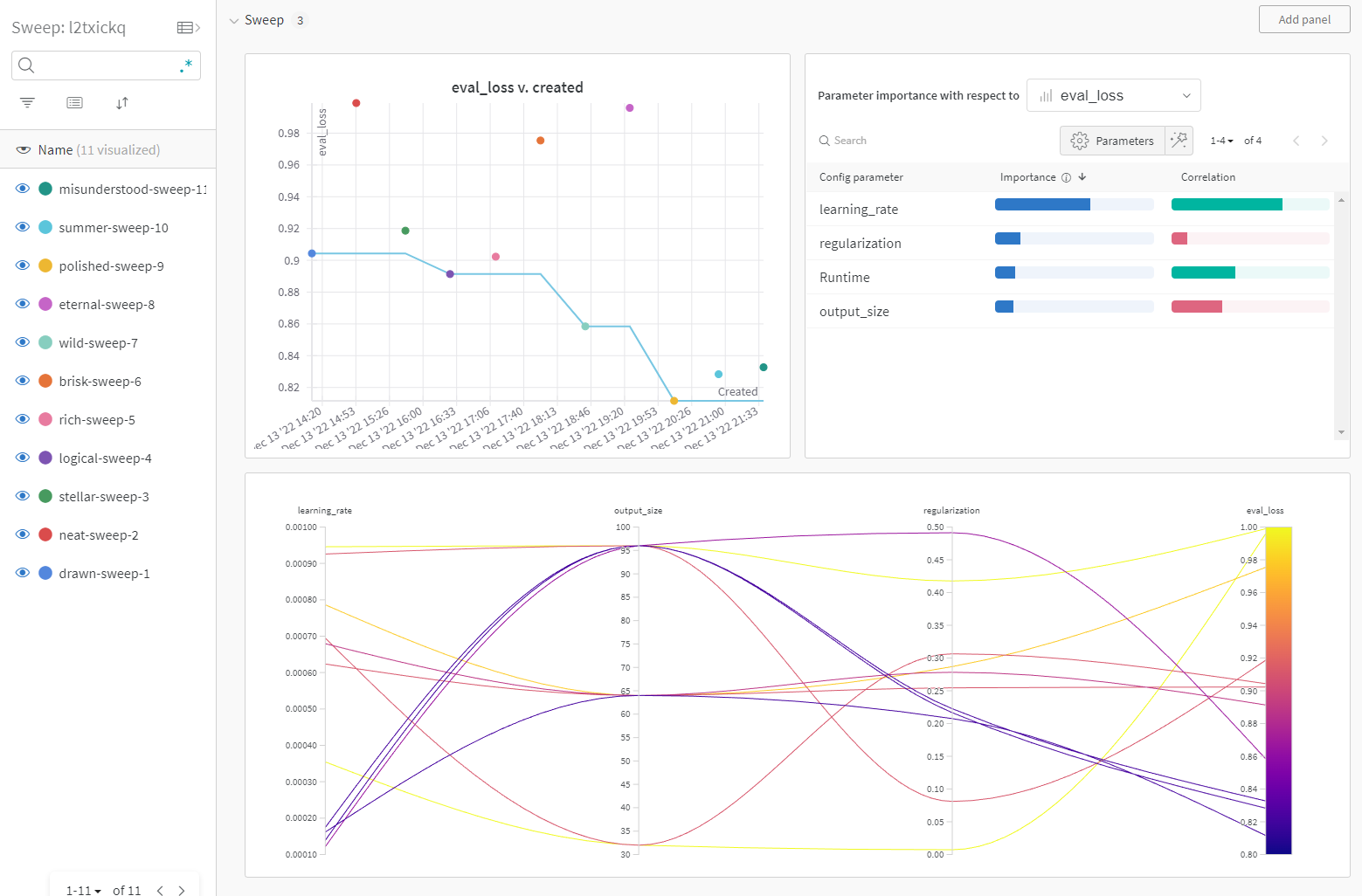
Figure 5-2. Weights and Biases Hyperparameter Sweep

In the Figure 5-2 you can see what a Weights and Biases Hyperparameter sweep looks like. On the left we have all the runs in the sweep, each run is trying a different set of values that we have specified in the config dictionary. In the middle we see how the final evaluation loss changes over time with the number of trials on the sweep and on the right we have a plot of how important the hyperparameter is in affecting the evaluation loss. Here we can see that the learning rate has the most effect on the eval loss, followed by the regularization amount.

On the bottom right of the figure we have a parallel coordinates plot of how each parameter affects the evaluation loss. The way to read it is to follow each line and see where it ends up on the final evaluation loss. The optimal hyperparameters can be found by tracing the line from the bottom right target value of evaluation loss back to the left through the values chosen for the hyperparameters. In this case the optimal value selected was a learning_rate of 0.0001618, a regularization of 0.2076 and an output_size of 64.

The rest of the code is mostly setting up the model and hooking up the input pipeline to model and deciding when to log metrics and model serialization and is mostly self explanatory. The details can be read in the Flax documentation.

In saving the model, notice that there are two different methods used. One is a checkpoint and the other is Flax serialization. The reason we have both is that the checkpoint is for when training jobs are cancelled and we need to recover the step that the job was cancelled at so we can resume training. The final serialization is for when the training is done. We also save a copy of the model as a Weights and Biases Artifact. The reason we do so is so that the Weights and Biases platform can keep track of the hyperparameters that created the model, the exact code and the exact githash that generated the model as well as providing a way to tell the lineage of the model. The lineage of the model consists of upstream artifacts used to generate the model (such as the training data), the state of the job used to create the model and adds a back link to all future jobs that might make use of the artifact. This makes it easier to reproduce models at a point in time or trace back what model was used and at what time in production. This comes in super handy when you have a larger organization and folks are hunting around for information on how a model was created. By using artifacts they can simply look in one place for the code and training data artifacts to reproduce a model.

Now that we have trained the models, we want to generate embeddings for the scene and the product database. The nice thing about using dot product as a scoring function as opposed to using a model is that you can generate scene and product embeddings independently and then scale it out at inference time. This kind of scaling will be introduced in the next putting it all together chapter, but for now the relevant part of the make_embeddings.py is as follows.

    model = models.STLModel(output_size=_OUTPUT_SIZE.value)
    state = None
    logging.info("Attempting to read model %s", _MODEL_NAME.value)
    with open(_MODEL_NAME.value, "rb") as f:
        data = f.read()
        state = flax.serialization.from_bytes(model, data)
    assert(state != None)

    @jax.jit
    def get_scene_embed(x):
      return model.apply(state["params"], x, method=models.STLModel.get_scene_embed)
    @jax.jit
    def get_product_embed(x):
      return model.apply(state["params"], x, method=models.STLModel.get_product_embed)

    ds = tf.data.Dataset
      .from_tensor_slices(unique_scenes)
      .map(input_pipeline.process_image_with_id)
    ds = ds.batch(_BATCH_SIZE.value, drop_remainder=True)
    it = ds.as_numpy_iterator()
    scene_dict = {}
    count = 0
    for id, image in it:
      count = count + 1
      if count % 100 == 0:
        logging.info("Created %d scene embeddings", count * _BATCH_SIZE.value)
      result = get_scene_embed(image)
      for i in range(_BATCH_SIZE.value):
        current_id = id[i].decode("utf-8")
        tmp = np.array(result[i])
        current_result = [float(tmp[j]) for j in range(tmp.shape[0])]
        scene_dict.update({current_id : current_result})
    scene_filename = os.path.join(_OUTDIR.value, "scene_embed.json")
    with open(scene_filename, "w") as scene_file:
      json.dump(scene_dict, scene_file)

As you can see we simply use the same Flax serialization library to load the model, and then call the appropriate method of the model using the apply function. We then save the vectors in a json file, since we have already been using json for the scene and product databases.

Finally, we’ll use the scoring code in make_recommendations.py to generate some product recommendations for sample scenes.

def find_top_k(
  scene_embedding,
  product_embeddings,
  k):
  """
  Finds the top K nearest product embeddings to the scene embedding.
  Args:
    scene_embedding: embedding vector for the scene
    product_embedding: embedding vectors for the products.
    k: number of top results to return.
  """

  scores = scene_embedding * product_embeddings
  scores = jnp.sum(scores, axis=-1)
  scores_and_indices = jax.lax.top_k(scores, k)
  return scores_and_indices

top_k_finder = jax.jit(find_top_k, static_argnames=["k"])

The most relevant code fragment is the scoring code where we have a scene embedding and we want to use Jax to score all the product embeddings vs a single scene embedding. Here we use Lax, a sub library of Jax that supplies direct API calls to XLA, the underlying machine learning compiler for Jax in order to access accelerated functions like top_k. In addition we compile the function find_top_k using jax’s jit. You can pass pure python functions that contain jax commands to jax.jit in order to compile them to a specific target architecture such as a GPU using XLA. Notice we have a special argument called static_argnames, this allows us to inform Jax that k is fixed and doesn’t change much so that Jax is able to compile a purpose built top_k_finder for a fixed value of k.

Here is a sample product recommendations for a scene where a woman is wearing a red shirt. The products recommended include some red velvent and some dark pants.

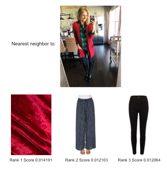
Figure 5-3. Recommended Items for Indoor Scene

Here is another scene where a woman is wearing a red coat outdoors and the matching accessories are a yellow handbag and a yellow long dress.

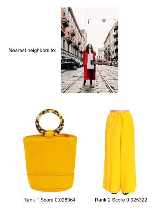
Figure 5-4. Recommended Items for an Outdoor Scene

We have pre-generated some results that are stored as an artifact that you can view by typing in the command below:

wandb artifact get building-recsys/recsys-pinterest/scene_product_results:v0

One thing you may notice is that the yellow bag and pants get recommended a lot. It may be possible that the embedding vector for the yellow bag is large, so it gets matched to a lot of scenes. This can be called the popular item problem and is a common issue with recommender systems. We will be covering some business logic to handle diversity and popularity in later chapters but is something that can happen with recommender systems that you might want to keep an eye out for.

And with that we conclude the first Putting It All Together chapter. If you haven’t played with the code yet, hop on over to to the GitHub repo give it a whirl! We hope that by giving a real world working example of an end to end content based recommender you will have a better feel of how the theory translates into practice. Enjoy playing with the code!