Chapter 8: Styles, ODS Options, and More
8.2 Style, Style Elements, and Attributes
8.3 Frequently Used ODS Options
8.4 Macro Variables, Dynamics, Conditionals, and Functions

A person who never made a mistake never tried
anything new. - Albert Einstein
The graphs that are created by GTL are aesthetic and effective by default. No fiddling with visual options or fonts is needed to get a good graph. GTL does this by using the ODS Styles associated with each open destination. A default style is associated with each ODS destination. These default styles contain the information that is needed to render each part of the output, including text, tables, and graphs.
As always, GTL also provides ways to change the visual appearance of the graph. You will learn about this topic in this chapter. We will also review the ODS GRAPHICS options that you can use to control the rendering of the graphs, and also the ODS destination options that are frequently used with graphs. Finally, you will learn how you can use advanced features such as dynamics, macro variables, conditionals, and function evaluation to make your graphs flexible and bulletproof.
8.1 Overview
A default style is associated with each ODS destination. For example, the default style for the SAS 9.3 HTML destination is called HTMLBLUE. Each style is a collection of style elements that contain the information needed to render a specific graphical element. The figure below shows a graph and some associated style element used to render it.

You can change the visual appearance of your graph in three different ways. You can use a different style (one supplied by SAS or one customized by you); you can assign different style elements to attribute options; or you can change the setting for a single attribute. We’ll cover this topic in Section 8.2.
You can control many aspects of the graph rendering by setting global options in the ODS Graphics statement or in the ODS destination statement. These options remain in effect for all the graphs that are created until the option is reset or changed. We will cover this topic in Section 8.3.
You can make your templates more flexible through the use of dynamics, macro variables, conditional syntax, and function evaluation. We will cover these topics in section 8.4.
8.2 Style, Style Elements, and Attributes

This is a graph of mean mileage by type. In this graph, you can change the visual attributes using all three approaches mentioned above.
1. Use STYLE=analysis on the ODS listing statement.
2. Specify that the fill attributes should come from the GRAPHDATA3 style element.
3. Specify that the fill transparency is set to 0.3
proc template;
define statgraph Fig_8_2;
begingraph;
entrytitle 'Mileage by Type';
layout overlay / xaxisopts=(display=(ticks tickvalues))
yaxisopts=(griddisplay=on);
barchart x=type y=mpg_city / stat=mean dataskin=gloss
fillattrs=graphdata3(transparency=0.3);
endlayout;
endgraph;
end;
run;
ods listing style=analysis;
proc sgrender template=Fig_8_2
data=sashelp.cars(where=(type ne 'Hybrid'));
run;
8.3 Frequently Used ODS Options
ODS Graphics Options
Many aspects of graph rendering can be controlled by using the options in the ODS Graphics statement. When you use the SGRENDER procedure for creating custom graphs, ODS Graphics is ON by default. The settings stay in effect until the option is reset or changed by a subsequent statement. Some common options are listed here. Please see the product documentation for details.
1. Graph WIDTH and HEIGHT specified in px, in, cm, and so on.
2. ANTIALIAS | NOANTIALIAS turns antialiasing on or off.
3. ANTIALIASMAX=number specifies the number of observations after which antialiasing is turned off. The default setting is 4000.
4. ATTRPRIORITY=AUTO | COLOR | NONE. Specifies if the graph data attributes are rotated with a color priority or not.
5. BORDER=ON | OFF controls the graph border.
6. DISCRETEMAX, GROUPMAX, PANELCELLMAX controls the maximum number of discrete or group values that are allowed or the number of cells that are allowed in a panel.
7. DRILLTARGET = ‘_BLANK” | “_SELF” | “frame-name” determines where the linked page is displayed.
8. IMAGEMAP turns on or off the creation of an image map for tooltips and URL drilldown in an HTML document.
9. IMAGENAME sets the filename of the output graph.
10. LABELMAX = n sets the number of labels after which collision avoidance is off.
11. MAXLEGENDAREAMAX = n sets the percent of graph space to be used for all legends.
12. OUTPUTFMT or IMAGEFMT – format for the output file.
13. TIPMAX sets the observation count after which tips are turned off.
14. RESET, SCALE, NOSCALE, SCALEMARKERS
ODS Destination Options
Some of the aspects of graph rendering are controlled by your choice of options in the ODS destination statement. The settings stay in effect until the option is reset or changed by a subsequent statement. Some common options are listed here. Please see the product documentation for details.
1. STYLE sets one of the SAS or user-defined styles for the destination.
2. IMAGE_DPI sets the dpi used for some destinations like LISTING and HTML.
3. FILE= filename sets the name of the file for some destinations.
4. PATH= sets the folder path for the output.
5. GPATH= sets the folder path for the graph output
6. URL=’location’ | NONE sets the URL path.
7. SGE=ON | OFF indicates whether an SGE graphics output should be created.
8.4 Macro Variables, Dynamics, Conditionals, and Functions
8.4.1 Macro Variables

Macro variables and numeric macro variables can be declared in the GTL syntax. They are used as parameter values that are evaluated at the time of creation of the graph, and not at compile time. This enables us to create templates that are flexible and that can be used in different cases. In this graph, _x and _y are declared as macro variables, and _degree is declared as a numeric macro variable (nmvar). Now, this template can be used for creating a fit plot for any pair of variable names that can be provided at run time.
proc template;
define statgraph Fig_8_4_2;
begingraph;
mvar _x _y;
nmvar _degree;
entrytitle _y ' by ' _x;
layout overlay / xaxisopts=(griddisplay=on)
yaxisopts=(griddisplay=on);
scatterplot x= _x y=_y;
regressionplot x= _x y=_y / degree=_degree;
endlayout;
endgraph;
end;
run;
%let _x=Horsepower;
%let _y=Mpg_City;
%let _degree=2;
proc sgrender template=Fig_8_4_2 data=sashelp.cars;
run;
8.4 2 Dynamics

You can declare dynamics in the GTL syntax. Dynamics are used as parameter values that are evaluated at the time of graph rendering, and not at compile time. This enables us to create templates that are flexible and that can be used in different cases.
In this graph, a DYNAMIC variable “_var” is declared and used in the syntax. When the template is compiled, this value is not resolved. At run time, in the SGRENDER procedure, the DYNAMIC statement is used to define the value for _val=’Horsepower’. Now, this template can be used for creating a distribution plot for any variable name that can be provided at run time.
proc template;
define statgraph Fig_8_4;
begingraph;
dynamic _var;
entrytitle 'Distribution of ' _var;
layout overlay / xaxisopts=(display=(ticks tickvalues))
yaxisopts=(griddisplay=on);
histogram _var / binaxis=false;
densityplot _var / kernel();
endlayout;
endgraph;
end;
run;
proc sgrender template=Fig_8_4 data=sashelp.cars;
dynamic _var='Horsepower';
run;
8.4.3 Conditionals

You can use the If-Else-Endif conditional block inside GTL to conditionally change the behavior of the template. In this graph, we have defined two dynamics _var and _type. We create a histogram of _var and overlay it with a density plot of _var, based on the value of _type. This is done by using the If-Else-Endif conditional block .
The If-Else-Endif conditional blocks can be nested inside the If or Else statements to build more complex conditions.
proc template;
define statgraph Fig_8_4_3;
begingraph;
dynamic _var _type;
entrytitle 'Distribution of ' _var;
layout overlay / xaxisopts=(display=(ticks tickvalues))
yaxisopts=(griddisplay=on);
histogram _var / binaxis=false;
if (_type = 'Kernel') densityplot _var / kernel();
else densityplot _var;
endif;
endlayout;
endgraph;
end;
run;
proc sgrender template=Fig_8_4_3 data=sashelp.cars;
dynamic _var='Horsepower' _type='Kernel';
run;
8.4.4 Function Evaluation
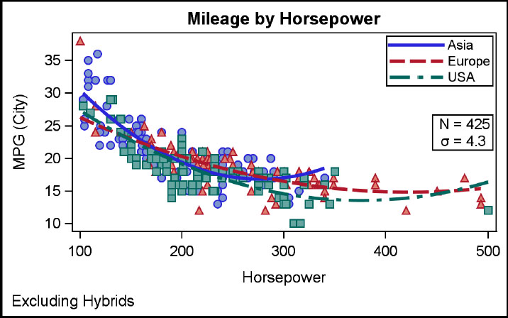
In the template, you can use any SAS or SGE function that returns a vector or a text string. (See the documentation for details.) Most data roles will accept a data set variable or expression. In this graph, the values for the statistic table are computed in the template using the eval syntax.
proc template; /*--SAS 9.4--*/
define statgraph Fig_8_4_4;
begingraph / datasymbols=(circlefilled trianglefilled squarefilled);
entrytitle 'Mileage by Horsepower';
entryfootnote halign=left 'Excluding Hybrids';
layout overlay;
scatterplot x=horsepower y=mpg_city / group=origin
filledoutlinedmarkers=true;
regressionplot x=horsepower y=mpg_city / degree=2 name='a'
group=origin lineattrs=(thickness=3);
layout gridded / rows=2 order=columnmajor border=true
autoalign=(right);
entry halign=right 'N = ';
entry halign=right {unicode SIGMA} ' =' ;
entry halign=left eval(strip(put(n(mpg_city),4.0)));
entry halign=left eval(strip(put(stddev(mpg_city),4.1)));
endlayout;
discretelegend 'a' 'b'/location=inside halign=right valign=top
across=1;
endlayout;
endgraph;
end; run;
proc sort data=sashelp.cars(where=(type ne 'Hybrid')) out=cars;
by origin; run;
proc sgrender template=Fig_8_4_4 data=cars; run;
8.5 Summary
In this chapter, you learned how to make your templates flexible and extensible by using styles, style elements, and style attributes. Using style elements and attributes enables you to use your template across different ODS destinations, without fear of a clash between colors of the various graph elements.
You also learned how to use the ODS Graphics and ODS Destination options to control the rendering of your graph.
Finally, you learned how to make your template flexible and extensible by use of macro variables, dynamics, function evaluation, and conditionals.
You can use these features to create graph templates that will stand the test of time.