
We are now entering the development stage. I will walk you through the coding of the application building blocks step-by-step. Logically, two core modules will be built, namely, Data Feed Provider and Stock Screener. First, we will build the Data Feed Provider.
The Data Feed Provider achieves the following three tasks:
- Collecting the historical stock quote data from Yahoo! Finance.
- Transforming the received data into a standardized format.
- Saving the standardized data into the Cassandra database.
Python has a well-known data analysis library called pandas. It is an open source library providing high-performance, easy-to-use data structures, and data analysis tools, especially, for time-series type of data. You can go to http://pandas.pydata.org/ for more details.
pandas offers a DataReader function in its pandas.io.data package. DataReader extracts financial data from various Internet sources into a data structure known as DataFrame. Yahoo! Finance is one of the supported Internet sources, making the collection of the historical stock quote data a piece of cake. Refer to the following Python code, cha
pter05_001.py:
# -*- coding: utf-8 -*-
# program: chapter05_001.py

## web is the shorthand alias of pandas.io.data
import pandas.io.data as web
import datetime

## we want to retrieve the historical daily stock quote of
## Goldman Sachs from Yahoo! Finance for the period
## between 1-Jan-2012 and 28-Jun-2014
symbol = 'GS'
start_date = datetime.datetime(2012, 1, 1)
end_date = datetime.datetime(2014, 6, 28)

## data is a DataFrame holding the daily stock quote
data = web.DataReader(symbol, 'yahoo', start_date, end_date)

## use a for-loop to print out the data
for index, row in data.iterrows():
    print index.date(), '	', row['Open'], '	', row['High'],
          '	', row['Low'], '	', row['Close'], '	', row['Volume']
A brief explanation is required. pandas offers a very handy data structure called DataFrame, which is a two-dimensional labeled data structure with columns of potentially different types. You can think of it as a spreadsheet or SQL table. It is generally the most commonly used pandas object.
The following is a screenshot demonstrating the use of Spyder to write and test chapter05_001.py code:
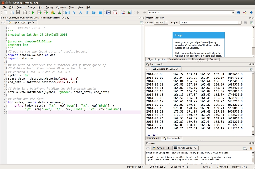
The left-hand side of the Spyder IDE is the place where you write Python code. The middle panel on the right-hand side is the IPython console that runs the code.
Along with the data in the DataFrame, you can optionally pass index (row labels) and columns (column labels). The row and column labels can be accessed respectively, by accessing the index and columns attributes. For example, you can revisit the screenshot of table.csv and see that the column names returned by Yahoo! Finance are Date, Open, High, Low, Close, Volume, and Adj Close, respectively. DataReader uses Date as the index of the returned DataFrame. The remaining column names become the column labels of the DataFrame.
The last for-loop in chapter05_001.py is also worth some remarks. DataFrame has a function, iterrows(), for iterating over its rows as (index, columns) pairs. Therefore, the for-loop uses iterrows() to iterate the daily stock quotes and we simply print out the index (that is converted to a string by the date() function), and the Open, High, Low, Close, Volume columns by passing the respective column labels to the row. Adj Close is a close price with adjustments of stock split, merge, and dividend. We do not use this, as we want to focus on pure prices.
Please be aware that stock quote data from the different sources might have different formats and, needless to say, different column names. Therefore, we need to take care of such a subtle difference, when mapping them to our standardized data model. DataFrame provides a very handy way to retrieve the data by column names and a few useful functions to manipulate the index and columns. We can make use of them to standardize the data format, as shown in chapter05_002.py:
# -*- coding: utf-8 -*-
# program: chapter05_002.py

## web is the shorthand alias of pandas.io.data
import pandas.io.data as web
import datetime

## we want to retrieve the historical daily stock quote of
## Goldman Sachs from Yahoo! Finance for the period
## between 1-Jan-2012 and 28-Jun-2014
symbol = 'GS'
start_date = datetime.datetime(2012, 1, 1)
end_date = datetime.datetime(2014, 6, 28)

## data is a DataFrame holding the daily stock quote
data = web.DataReader(symbol, 'yahoo', start_date, end_date)

## standardize the column names
## rename index column to price_date to match the Cassandra table
data.index.names=['price_date']

## drop extra column 'Adj Close'
data = data.drop(['Adj Close'], axis=1)

## rename the columns to match the respective columns in Cassandra
data = data.rename(columns={'Open':'open_price',
                            'High':'high_price',
                            'Low':'low_price',
                            'Close':'close_price',
                            'Volume':'volume'})

## use a for-loop to print out the transformed data
for index, row in data.iterrows():
    print index.date(), '	', row['open_price'], '	',
                              row['high_price'], '	',
                              row['low_price'], '	',
                              row['close_price'], '	',
row['volume']Before storing the retrieved data in Cassandra, we need to create the keyspace and table in the Cassandra database. We will create a keyspace called packtcdma and a table called quote in chapter05_003.py to hold the Historical Data, as shown in the following code:
# -*- coding: utf-8 -*-
# program: chapter05_003.py

## import Cassandra driver library
from cassandra.cluster import Cluster

## create Cassandra instance
cluster = Cluster()

## establish Cassandra connection, using local default
session = cluster.connect()

## create keyspace packtcdma if not exists
## currently it runs on a single-node cluster
session.execute("CREATE KEYSPACE IF NOT EXISTS packtcdma " +
                "WITH replication" +
                "={'class':'SimpleStrategy', " +
                "'replication_factor':1}")

## use packtcdma keyspace
session.set_keyspace('packtcdma')

## execute CQL statement to create quote table if not exists
session.execute('CREATE TABLE IF NOT EXISTS quote (' +
                'symbol varchar,' +
                'price_time timestamp,' +
                'open_price float,' +
                'high_price float,' +
                'low_price float,' +
                'close_price float,' +
                'volume double,' +
                'PRIMARY KEY (symbol, price_time))')

## close Cassandra connection
cluster.shutdown()
The comments of the code are sufficient to explain what it is doing. Now, we have the Historical Data repository ready and what follows is to store the received data into it. This is exactly the purpose of chapter05_004.py in which a Python function is created to insert the data, as shown in the following code:
# -*- coding: utf-8 -*-
# program: chapter05_004.py

## import Cassandra driver library
from cassandra.cluster import Cluster
from decimal import Decimal

## function to insert historical data into table quote
## ss: Cassandra session
## sym: stock symbol
## d: standardized DataFrame containing historical data
def insert_quote(ss, sym, d):
    ## CQL to insert data, ? is the placeholder for parameters
    insert_cql = 'INSERT INTO quote (' +
                 'symbol, price_time, open_price, high_price,' +
                 'low_price, close_price, volume' +
                 ') VALUES (' +
                 '?, ?, ?, ?, ?, ?, ?' +
                 ')'
    ## prepare the insert CQL as it will run repeatedly
    insert_stmt = ss.prepare(insert_cql)

    ## set decimal places to 4 digits
    getcontext().prec = 4

    ## loop thru the DataFrame and insert records
    for index, row in d.iterrows():
        ss.execute(insert_stmt,
                   [sym, index,
                   Decimal(row['open_price']),
                   Decimal(row['high_price']),
                   Decimal(row['low_price']),
                   Decimal(row['close_price']),
                   Decimal(row['volume'])
                   ])
Although chapter05_004.py contains less than ten lines of code, it is rather complicated and needs some explanation.
We can create a function in Python using the keyword def. This must be followed by the function name and the parenthesized list of formal parameters. The code that form the body of the function starts in the next line, indented by a tab. Thus, in chapter05_004.py, the function name is insert_quote() with three parameters, namely, ss, sym, and d.
Note
Indentation in Python
In Python, leading whitespace (spaces and tabs) at the beginning of a logical line is used to compute the indentation level of the line, which in turn is used to determine the grouping of statements. Be very careful of this. Most of the Python IDE has features to check against the indentations. The article on the myths about indentation of Python is worth reading, which is available at http://www.secnetix.de/olli/Python/block_indentation.hawk.
The second interesting thing is the prepare() function. It is used to prepare CQL statements that are parsed by Cassandra and then saved for later use. When the driver uses a prepared statement, it only needs to send the values of parameters to bind. This lowers network traffic and CPU utilization as a result of the avoidance of re-parsing the statement each time.
The placeholders for prepared statements are ? characters so that the parameters are passed in sequence. This method is called positional parameter passing.
The last segment of code is a for-loop that iterates through the DataFrame and inserts each row into the quote table. We also use the Decimal() function to cast the string into numeric value.
All pieces of Python code can be combined to make the Data Feed Provider. To make the code cleaner, the code fragment for the collection of stock quote is encapsulated in a function called collect_data() and that for data transformation in transform_yahoo() function. The complete program, chapter05_
005.py, is listed as follows:.
# -*- coding: utf-8 -*-
# program: chapter05_005.py

## import Cassandra driver library
from cassandra.cluster import Cluster
from decimal import Decimal

## web is the shorthand alias of pandas.io.data
import pandas.io.data as web
import datetime

## function to insert historical data into table quote
## ss: Cassandra session
## sym: stock symbol
## d: standardized DataFrame containing historical data
def insert_quote(ss, sym, d):
    ## CQL to insert data, ? is the placeholder for parameters
    insert_cql = "INSERT INTO quote (" +
                 "symbol, price_time, open_price, high_price," +
                 "low_price, close_price, volume" +
                 ") VALUES (" +
                 "?, ?, ?, ?, ?, ?, ?" +
                 ")"
    ## prepare the insert CQL as it will run repeatedly
    insert_stmt = ss.prepare(insert_cql)

    ## set decimal places to 4 digits
    getcontext().prec = 4

    ## loop thru the DataFrame and insert records
    for index, row in d.iterrows():
        ss.execute(insert_stmt,
                   [sym, index,
                   Decimal(row['open_price']),
                   Decimal(row['high_price']),
                   Decimal(row['low_price']),
                   Decimal(row['close_price']),
                   Decimal(row['volume'])
                   ])

## retrieve the historical daily stock quote from Yahoo! Finance
## Parameters
## sym: stock symbol
## sd: start date
## ed: end date
def collect_data(sym, sd, ed):
    ## data is a DataFrame holding the daily stock quote
    data = web.DataReader(sym, 'yahoo', sd, ed)
    return data

## transform received data into standardized format
## Parameter
## d: DataFrame containing Yahoo! Finance stock quote
def transform_yahoo(d):
    ## drop extra column 'Adj Close'
    d1 = d.drop(['Adj Close'], axis=1)

    ## standardize the column names
    ## rename index column to price_date
    d1.index.names=['price_date']

    ## rename the columns to match the respective columns
    d1 = d1.rename(columns={'Open':'open_price',
                            'High':'high_price',
                            'Low':'low_price',
                            'Close':'close_price',
                            'Volume':'volume'})
    return d1

## create Cassandra instance
cluster = Cluster()

## establish Cassandra connection, using local default
session = cluster.connect('packtcdma')

symbol = 'GS'
start_date = datetime.datetime(2012, 1, 1)
end_date = datetime.datetime(2014, 6, 28)

## collect data
data = collect_data(symbol, start_date, end_date)

## transform Yahoo! Finance data
data = transform_yahoo(data)

## insert historical data
insert_quote(session, symbol, data)

## close Cassandra connection
cluster.shutdown()The Stock Screener retrieves historical data from the Cassandra database and applies technical analysis techniques to produce alerts. It has four components:
- Retrieve historical data over a specified period
- Program a technical analysis indicator for time-series data
- Apply the screening rule to the historical data
- Produce alert signals
To utilize technical analysis techniques, a sufficient optimal number of stock quote data is required for calculation. We do not need to use all the stored data, and therefore a subset of data should be retrieved for processing. The following code, chapte05_006.py, retrieves the historical data from the table quote within a specified period:
# -*- coding: utf-8 -*-
# program: chapter05_006.py

import pandas as pd
import numpy as np

## function to insert historical data into table quote
## ss: Cassandra session
## sym: stock symbol
## sd: start date
## ed: end date
## return a DataFrame of stock quote
def retrieve_data(ss, sym, sd, ed):
    ## CQL to select data, ? is the placeholder for parameters
    select_cql = "SELECT * FROM quote WHERE symbol=? " + "AND price_time >= ? AND price_time <= ?"

    ## prepare select CQL
    select_stmt = ss.prepare(select_cql)

    ## execute the select CQL
    result = ss.execute(select_stmt, [sym, sd, ed])

    ## initialize an index array
    idx = np.asarray([])

    ## initialize an array for columns
    cols = np.asarray([])

    ## loop thru the query resultset to make up the DataFrame
    for r in result:
        idx = np.append(idx, [r.price_time])
        cols = np.append(cols, [r.open_price, r.high_price,
.low_price, r.close_price, r.volume])

    ## reshape the 1-D array into a 2-D array for each day
    cols = cols.reshape(idx.shape[0], 5)

    ## convert the arrays into a pandas DataFrame
    df = pd.DataFrame(cols, index=idx,
                      columns=['close_price', 'high_price',
                      'low_price', 'close_price', 'volume'])
    return df
The first portion of the function should be easy to understand. It executes a select_cql query for a particular stock symbol over a specified date period. The clustering column, price_time, makes range query possible here. The query result set is returned and used to fill two NumPy arrays, idx for index, and cols for columns. The cols array is then reshaped as a two-dimensional array with rows of prices and volume for each day. Finally, both idx and cols arrays are used to create a DataFrame to return df.
As a simple illustration, we use a 10-day
Simple Moving Average (SMA) as the technical analysis signal for stock screening. pandas provides a rich set of functions to work with time-series data. The SMA can be easily computed by the rolling_mean() function, as shown in chapter05_007.py:
# -*- coding: utf-8 -*-
# program: chapter05_007.py

import pandas as pd

## function to compute a Simple Moving Average on a DataFrame
## d: DataFrame
## prd: period of SMA
## return a DataFrame with an additional column of SMA
def sma(d, prd):
    d['sma'] = pd.rolling_mean(d.close_price, prd)
return dWhen SMA is calculated, we can apply a screening rule in order to look for trading signals. A very simple rule is adopted: a buy-and-hold signal is generated whenever a trading day whose close price is higher than 10-day SMA. In Python, it is just a one liner by virtue of pandas power. Amazing! Here is an example:
# -*- coding: utf-8 -*-
# program: chapter05_008.py

## function to apply screening rule to generate buy signals
## screening rule, Close > 10-Day SMA
## d: DataFrame
## return a DataFrame containing buy signals
def signal_close_higher_than_sma10(d):
return d[d.close_price > d.sma]Until now, we coded the components of the Stock Screener. We now combine them together to generate the Alert List, as shown in the following code:
# -*- coding: utf-8 -*-
# program: chapter05_009.py

## import Cassandra driver library
from cassandra.cluster import Cluster

import pandas as pd
import numpy as np
import datetime

## function to insert historical data into table quote
## ss: Cassandra session
## sym: stock symbol
## sd: start date
## ed: end date
## return a DataFrame of stock quote
def retrieve_data(ss, sym, sd, ed):
    ## CQL to select data, ? is the placeholder for parameters
    select_cql = "SELECT * FROM quote WHERE symbol=? " + "AND price_time >= ? AND price_time <= ?"

    ## prepare select CQL
    select_stmt = ss.prepare(select_cql)

    ## execute the select CQL
    result = ss.execute(select_stmt, [sym, sd, ed])

    ## initialize an index array
    idx = np.asarray([])

    ## initialize an array for columns
    cols = np.asarray([])

    ## loop thru the query resultset to make up the DataFrame
    for r in result:
        idx = np.append(idx, [r.price_time])
        cols = np.append(cols, [r.open_price, r.high_price,
                         r.low_price, r.close_price, r.volume])

    ## reshape the 1-D array into a 2-D array for each day
    cols = cols.reshape(idx.shape[0], 5)

    ## convert the arrays into a pandas DataFrame
    df = pd.DataFrame(cols, index=idx,
                      columns=['open_price', 'high_price',
                      'low_price', 'close_price', 'volume'])
    return df

## function to compute a Simple Moving Average on a DataFrame
## d: DataFrame
## prd: period of SMA
## return a DataFrame with an additional column of SMA
def sma(d, prd):
    d['sma'] = pd.rolling_mean(d.close_price, prd)
    return d

## function to apply screening rule to generate buy signals
## screening rule, Close > 10-Day SMA
## d: DataFrame
## return a DataFrame containing buy signals
def signal_close_higher_than_sma10(d):
    return d[d.close_price > d.sma]

## create Cassandra instance
cluster = Cluster()

## establish Cassandra connection, using local default
session = cluster.connect('packtcdma')
## scan buy-and-hold signals for GS over 1 month since 28-Jun-2012
symbol = 'GS'
start_date = datetime.datetime(2012, 6, 28)
end_date = datetime.datetime(2012, 7, 28)

## retrieve data
data = retrieve_data(session, symbol, start_date, end_date)

## close Cassandra connection
cluster.shutdown()

## compute 10-Day SMA
data = sma(data, 10)

## generate the buy-and-hold signals
alerts = signal_close_higher_than_sma10(data)

## print out the alert list
for index, r in alerts.iterrows():
    print index.date(), '	', r['close_price']