
We will initialize t just as in the previous section. We need to sum a number of terms. The higher the number of terms, the more accurate the result; k = 99 should be sufficient. In order to draw a square wave, follow these steps:
- We will start by initializing
tandk. Set the initial values for the function to0:t = np.linspace(-np.pi, np.pi, 201) k = np.arange(1, 99) k = 2 * k - 1 f = np.zeros_like(t)
- Compute the function values with the
sin()andsum()functions:for i, ti in enumerate(t): f[i] = np.sum(np.sin(k * ti)/k) f = (4 / np.pi) * f
- The code to plot is almost identical to the one in the previous section:
plt.plot(t, f) plt.title('Square wave') plt.grid() plt.show()The resulting square wave generated with
k=99is as follows: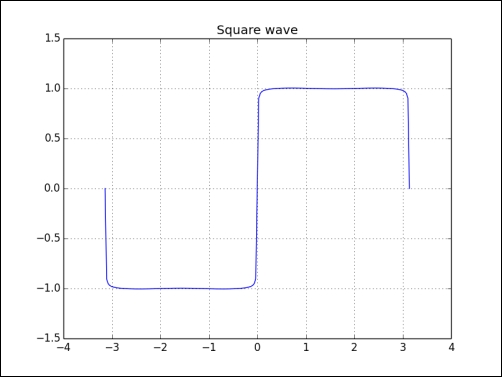
We generated a square wave or, at least, a fair approximation of it, using the sin() function. The input values were assembled with the linspace() function and the k values with the arange() function (see squarewave.py):
import numpy as np
import matplotlib.pyplot as plt
t = np.linspace(-np.pi, np.pi, 201)
k = np.arange(1, 99)
k = 2 * k - 1
f = np.zeros_like(t)
for i, ti in enumerate(t):
   f[i] = np.sum(np.sin(k * ti)/k)

f = (4 / np.pi) * f
plt.plot(t, f)
plt.title('Square wave')
plt.grid()
plt.show()..................Content has been hidden....................
You can't read the all page of ebook, please click here login for view all page.