
Let's plot a polynomial and its first and second derivative. We will make three subplots for the sake of clarity:
- Create a polynomial and its derivatives using the following code:
func = np.poly1d(np.array([1, 2, 3, 4]).astype(float))
x = np.linspace(-10, 10, 30)
y = func(x)
func1 = func.deriv(m=1)
y1 = func1(x)
func2 = func.deriv(m=2)
y2 = func2(x)
- Create the first subplot of the polynomial with the
subplot()function. The first parameter of this function is the number of rows, the second parameter is the number of columns, and the third parameter is an index number starting with 1. Alternatively, combine the three parameters into a single number, such as311. The subplots will be organized in three rows and one column. Give the subplot the title Polynomial. Make a solid red line:plt.subplot(311) plt.plot(x, y, 'r-') plt.title("Polynomial") - Create the third subplot of the first derivative with the
subplot()function. Give the subplot the title First Derivative. Use a line of blue triangles:plt.subplot(312) plt.plot(x, y1, 'b^') plt.title("First Derivative") - Create the second subplot of the second derivative with the
subplot()function. Give the subplot the title Second Derivative. Use a line of green circles:plt.subplot(313) plt.plot(x, y2, 'go') plt.title("Second Derivative") plt.xlabel('x') plt.ylabel('y') plt.show()The three subplots with polynomial coefficients 1, 2, 3, and 4 are as follows:
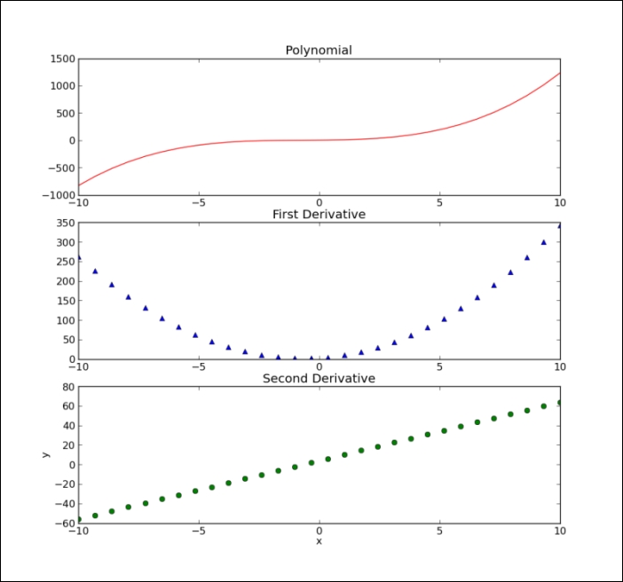
We plotted a polynomial and its first and second derivatives using three different line styles and three subplots in three rows and one column (see polyplot3.py):
import numpy as np
import matplotlib.pyplot as plt
func = np.poly1d(np.array([1, 2, 3, 4]).astype(float))
x = np.linspace(-10, 10, 30)
y = func(x)
func1 = func.deriv(m=1)
y1 = func1(x)
func2 = func.deriv(m=2)
y2 = func2(x)
plt.subplot(311)
plt.plot(x, y, 'r-')
plt.title("Polynomial")
plt.subplot(312)
plt.plot(x, y1, 'b^')
plt.title("First Derivative")
plt.subplot(313)
plt.plot(x, y2, 'go')
plt.title("Second Derivative")
plt.xlabel('x')
plt.ylabel('y')
plt.show()..................Content has been hidden....................
You can't read the all page of ebook, please click here login for view all page.