
Keeping an open mind, let's assume that we can express a stock price p as a linear combination of previous values, that is, a sum of those values multiplied by certain coefficients we need to determine:

In linear algebra terms, this boils down to finding a least-squares method (see https://www.khanacademy.org/math/linear-algebra/alternate_bases/orthogonal_projections/v/linear-algebra-least-squares-approximation).
Note
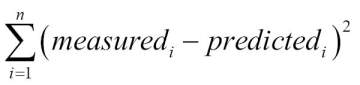
Independently of each other, the astronomers Legendre and Gauss created the least squares method around 1805 (see http://en.wikipedia.org/wiki/Least_squares). The method was initially used to analyze the motion of celestial bodies. The algorithm minimizes the sum of the squared residuals (the difference between measured and predicted values):
- First, form a vector
bcontainingNprice values:b = c[-N:] b = b[::-1] print("b", x)The result is as follows:
b [ 351.99 346.67 352.47 355.76 355.36] - Second, pre-initialize the matrix
Ato beN-by-Nand contain zeros:A = np.zeros((N, N), float) Print("Zeros N by N", A)The following should be printed on your screen:
Zeros N by N [[ 0.  0.  0.  0.  0.]
 [ 0.  0.  0.  0.  0.]
 [ 0.  0.  0.  0.  0.]
 [ 0.  0.  0.  0.  0.]
 [ 0.  0.  0.  0.  0.]]
- Third, fill the matrix
AwithNpreceding price values for each value inb:for i in range(N): A[i, ] = c[-N - 1 - i: - 1 - i] print("A", A)Now,
Alooks like this:A [[ 360. 355.36 355.76 352.47 346.67] [ 359.56 360. 355.36 355.76 352.47] [ 352.12 359.56 360. 355.36 355.76] [ 349.31 352.12 359.56 360. 355.36] [ 353.21 349.31 352.12 359.56 360. ]]
- The objective is to determine the coefficients that satisfy our linear model by solving the least squares problem. Employ the
lstsq()function of the NumPylinalgpackage to do this:(x, residuals, rank, s) = np.linalg.lstsq(A, b) print(x, residuals, rank, s)
The result is as follows:
[ 0.78111069 -1.44411737 1.63563225 -0.89905126 0.92009049] [] 5 [ 1.77736601e+03 1.49622969e+01 8.75528492e+00 5.15099261e+00 1.75199608e+00]The tuple returned contains the coefficient
xthat we were after, an array comprising residuals, the rank of matrixA, and the singular values ofA. - Once we have the coefficients of our linear model, we can predict the next price value. Compute the dot product (with the NumPy
dot()function) of the coefficients and the last knownNprices:print(np.dot(b, x))
The dot product (see https://www.khanacademy.org/math/linear-algebra/vectors_and_spaces/dot_cross_products/v/vector-dot-product-and-vector-length) is the linear combination of the coefficients
band the pricesx. As a result, we get:357.939161015
I looked it up; the actual close price of the next day was 353.56. So, our estimate with N = 5 was not that far off.
We predicted tomorrow's stock price today. If this works in practice, we can retire early! See, this book was a good investment, after all! We designed a linear model for the predictions. The financial problem was reduced to a linear algebraic one. NumPy's linalg package has a practical lstsq() function that helped us with the task at hand, estimating the coefficients of a linear model. After obtaining a solution, we plugged the numbers in the NumPy dot() function that presented us an estimate through linear regression (see linearmodel.py):
from __future__ import print_function
import numpy as np
N = 5
c = np.loadtxt('data.csv', delimiter=',', usecols=(6,), unpack=True)
b = c[-N:]
b = b[::-1]
print("b", b)
A = np.zeros((N, N), float)
print("Zeros N by N", A)
for i in range(N):
   A[i, ] = c[-N - 1 - i: - 1 - i]

   print("A", A)
(x, residuals, rank, s) = np.linalg.lstsq(A, b)

print(x, residuals, rank, s)
print(np.dot(b, x))