
Let's understand the core concepts of Spark in this section. The main abstraction Spark provides is a Resilient Distributed Dataset (RDD). So, let's understand what an RDD is and operations in RDDs that provide in-memory performance and fault tolerance. But, let's learn the ways to work with Spark first.
There are a couple of ways to work with Spark—Spark Shell and Spark Applications.
Interactive REPL (read-eval-print loop) for data exploration using Scala, Python, or R:
// Entering to Scala Shell . :q to exit the shell.
[cloudera@quickstart spark-2.0.0-bin-hadoop2.7]$ bin/spark-shell

# Entering to Python Shell. ctrl+d to exit the shell.
[cloudera@quickstart spark-2.0.0-bin-hadoop2.7]$ bin/pyspark

// Entering to R Shell. Need to install R first. ctrl+d to exit shell
[cloudera@quickstart spark-2.0.0-bin-hadoop2.7]$ bin/sparkR
For a complete list of spark-shell options, use the following command.
[cloudera@quickstart spark-2.0.0-bin-hadoop2.7]$ bin/spark-shell help
Usage: ./bin/spark-shell [options]
The Scala shell provides lots of utilities and tab completion for ease of use. Some of these useful utilities are shown in the following examples.
Executing system commands and checking return code:
import sys.process._
val res = "ls /tmp" ! // notice the "!" operator
println("result = "+res) // result can be zero or non-zero
Executing system commands and checking output:
import sys.process._
val output = "hadoop fs -ls" !! // notice the "!!" operator
println("result = "+output)
Pasting spark code lines in the shell:
:paste
// Entering paste mode (ctrl-D to finish)
To exit from the Scala shell use the :q command.
Entering the Scala shell by passing a set of commands to run:
[root@myhost ~]# spark-shell -i spark_commands.txt
Enter the Scala shell, execute commands, and exit:
[root@myhost ~]# cat spark_commands.txt | spark-shell
The Python shell does not provide tab completion but iPython notebook provides tab completion.
While the Spark shell is used for development and testing, Spark applications are used for creating and scheduling large scale data processing applications in production. Applications can be created in natively-supported languages such as Python, Scala, Java, SQL, R, or external programs using the pipe method. Spark-submit is used for submitting a spark application as shown in the following Scala-based application example:
[root@myhost ~]# spark-submit
  --class com.example.loganalytics.MyApp
  --master yarn
  --name "Log Analytics Application"
  --executor-memory 2G
  --num-executors 50
  --conf spark.shuffle.spill=false
  myApp.jar
  /data/input
  /data/output

Spark-submit for Python based application.

[root@myhost ~]# spark-submit --master yarn-client myapp.py
The user can acquire a Kerberos ticket with the kinit command to work with shells or applications. For applications submitting spark jobs, use the klist command to display the principals of the spark keytab as shown in the following:
klist -ket /path/to/spark.keytab
Use the kinit command with keytab and principal to get a ticket as shown in the following:
kinit -kt /path/to/spark.keytab principal_name
Once the ticket is acquired, the application should be able to connect to the Spark cluster using a shell or application.
You can also pass the --keytab and --principal options with spark-submit when using YARN as the resource manager.
RDDs are a fundamental unit of data in Spark and Spark programming revolves around creating and performing operations on RDDs. They are immutable collections partitioned across clusters that can be rebuilt (re-computed) if a partition is lost. They are created by transforming data in a stable storage using data flow operators (map, filter, group-by) and can be cached in memory across parallel operations:
- Resilient: If data in memory is lost, it can be recreated (or recomputed)
- Distributed: Distributed across clusters
- Dataset: Initial data can come from a file or created programmatically
There are a couple of ways to create an RDD: parallelize, or read from a file:
Take an existing in-memory collection of data and pass it to SparkContext's parallelize method. This is not generally used in production systems but used for prototyping and testing since it requires an entire dataset in memory on one machine.
Examples of creating an RDD using the parallelize method:
// Parallelize a list in Java
JavaRDD<String> myRDD = sc.parallelize(Arrays.asList("hdfs", "spark", "rdd"));

# Parallelize a list in Python
myRDD = sc.parallelize(["hdfs", "spark", "rdd"])

// Parallelize a list in Scala
val myRDD= sc.parallelize(List("hdfs", "spark", "rdd"))The second method is to read data from HDFS, S3, HBase, Avro, a Parquet file, and other Hadoop-supported formats. Input can be a file or a directory. Wildcards are supported as well.
Example of creating a RDD called as inputRDD by reading an input file:
// Read a file in Java
JavaRDD<String> inputRDD = sc.textFile("/path/to/input");

# Read a file in Python
inputRDD = sc.textFile("/path/to/input")

// Read a file in Scala
val inputRDD = sc.textFile("/path/to/input")There are a couple of ways for reading files from HDFS.
The first method is to specify the HDFS URI with namenode hostname and RPC port number:
// Read a HDFS file in Scala
val inputRDD = sc.textFile("hdfs://namenodehostname:8020/data/input")
The second method is to set and specify the HADOOP_CONF_DIR environment variable in spark-env.sh and specify the path directly:
// Read a HDFS file in Scala
val inputRDD = sc.textFile("/data/input")
HADOOP_CONF_DIR can be set in /etc/spark/conf/spark-env.sh or you can add Hadoop configuration files to the spark configuration directory.
SparkContext.textFile calls org.apache.hadoop.mapred.FileInputFormat.getSplits which in turn uses org.apache.hadoop.fs.getDefaultUri. This method reads the fs.defaultFS parameter of Hadoop conf (core-site.xml).
Every Spark application requires a Spark context, which is the main entry point to the Spark RDD API. The Spark shell provides a pre-configured Spark context called "sc" and a pre-configured Spark session called "spark" as shown in the following screenshot (Figure 3.1):

Figure 3.1: Spark context "sc" in Spark shell.
In Spark applications, SparkContext must be created first as shown in the following Scala code. To create a SparkContext object, build a SparkConf object that has the information about the application. Only one SparkContext is created per application:
val conf = new SparkConf().setAppName("App1").setMaster("yarn")
val mysc = new SparkContext(conf)
val an = mysc.appName
println("App Name = "+an)
Output of this application: App Name = App1There are two types of RDD operations—transformations and actions. Transformations define new RDDs based on the current RDD. Actions return values from RDDs.
Let's go through some examples of transformations and actions with visualizations to understand them better.
Figure 3.2 shows how a sample text file is read (using the Python code) to create a base RDD called fileRDD, transformed with the 'map' transformation to create upperRDD. Finally, upperRDD is filtered with the 'filter' transformation and output is generated with the 'collect' action. Transformations do not cause any execution until they see an action. So, Transformations are lazily evaluated and actions kick off the job to execute all transformations. In this example, the actual job execution starts from line number 3 because of the 'collect' action.
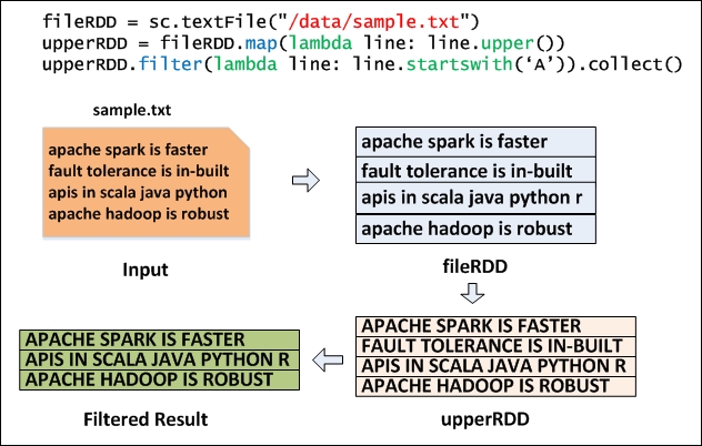
Figure 3.2: Map and Filter Transformation using Python.
In the preceding example, we have seen how the data is transformed and the action produced the result. Let's deep dive to understand what exactly is happening internally with a Log Analytics example using the Python language:
access_log = sc.textFile("hdfs://...")
#Filter Lines with ERROR only
error_log = access_log.filter(lambda x: "ERROR" in x)
# Cache error log in memory
cached_log = error_log.cache()
# Now perform an action -  count
print "Total number of error records are %s" % (cached_log.count())
# Now find the number of lines with
print "Number of product pages visited that have Errors is %s" % (cached_log.filter(lambda x: "product" in x).count())
Figure 3.3 explains the log analytics example.

Figure 3.3: Log analytics flow
The log analytics example is reading files from a HDFS directory with three blocks (B1, B2, and B3) and creating a base RDD called access_log. The base RDD is then filtered to create error_log RDD that contains records with ERROR. Error_log RDD is cached in memory with the RDD name cached_log. A couple of actions are performed on cached_log RDD. As actions cause transformations to be executed, the first action will create access_log, error_log and cached_log and then the result is sent to the client. The second action will not create the access_log, error_log, and cached_log. It will directly read data from cached_log. So, the performance of the second action will be much faster than the first action. It is always recommended to cache data if more than one action is to be performed on the same RDD. Caching can be done at any point in the program. For example, caching can be done directly after creating the base RDD access_log. But, in this case, you will be storing a huge amount of data in the cache. So, it's always recommended to filter out data that is not needed and then cache it. RDDs that are not cached are garbage collected. So, in the log analytics example, access_log and error_log RDDs are garbage collected.
Parallelism in RDDs is controlled by a spark.default.parallelism parameter. This defaults to the total number of cores on executors or 2, whichever is larger. Let's understand this by looking at the following example.
Enter the python shell using the pyspark command and then check the default parallelism as shown in the following. Assuming that that the default number of cores available on your cluster is eight:
[cloudera@quickstart spark-2.0.0-bin-hadoop2.7]$ bin/pyspark --master spark://quickstart.cloudera:7077
>>> sc.defaultParallelism
8
But, if you enter the spark shell using the following command, the default parallelism will be the same as the number of cores allocated:
[cloudera@quickstart spark-2.0.0-bin-hadoop2.7]$ bin/pyspark --master spark://quickstart.cloudera:7077 --total-executor-cores 4
For local mode:
[cloudera@quickstart spark-2.0.0-bin-hadoop2.7]$ bin/pyspark --master local[4]


>>> sc.defaultParallelism
4
Let's create a list, parallelize it, and check the number of partitions:
>>> myList = ["big", "data", "analytics", "hadoop" , "spark"]
>>> myRDD = sc.parallelize(myList)
>>> myRDD.getNumPartitions()
This defaults to the same value as sc.defaultParallelism
To override the default parallelism, provide the specific number of partitions needed while creating the RDD. In this case, let's create the RDD with six partitions:
>>> myRDDWithMorePartitions = sc.parallelize(myList,6)
>>> myRDDWithMorePartitions.getNumPartitions()
6
Let's issue an action to count the number of elements in the list:
>>> myRDD.count()
5
The getNumPartitions() method shows that myRDD has four partitions in it. So, any action on this RDD would need four tasks. This means that in order to compute a .count() action, the Driver JVM shipped out the 'counting code' to four tasks (threads) running on different machines. Each task/thread reads and counts the data from only one partition and sends the results back to the Driver JVM. The driver then aggregates all four counts into a final answer. This can be visualized by looking at Spark's UI:
Spark's UI address: http://masterhostname:8080
Click on the application ID under Running Applications and then Application Detail UI which will take you to the UI http://masterhostname:4040/jobs/. You can see that four tasks are created for this action as shown in Figure 3.4. We can see the other details by clicking on the Environment and Executors tabs. The Storage tab will show the cached RDDs with the percentage cached and size of the data cached.

Figure 3.4: UI showing four tasks for four partitions.
If you click on the completed job, you can see the task duration, executor ID, hostname, and other details as shown in Figure 3.5.

Figure 3.5: UI showing task duration.
Now, the mapPartitionsWithIndex() transformation uses a lambda function that takes in a partition index (like the partition number) and an iterator (to the items in that specific partition). For every partition index + iterator pair that goes in, the lambda function returns a tuple of the same partition index number and also a list of the actual items in that partition:
>>> myRDD.mapPartitionsWithIndex(lambda index,iterator: ((index, list(iterator)),)).collect()

[(0, ['big']), (1, ['data']), (2, ['analytics']), (3, ['hadoop', 'spark'])]
The preceding result explains how the list is distributed across the partitions of the RDD. Let's increase the number of partitions now and see how data is re-distributed to partitions of the new RDD.
>>> mySixPartitionsRDD = myRDD.repartition(6)
>>> mySixPartitionsRDD.mapPartitionsWithIndex(lambda index,iterator: ((index, list(iterator)),)).collect()

[(0, []), (1, ['big']), (2, []), (3, ['hadoop']), (4, ['data', 'spark']), (5, ['analytics'])]
Now, it's interesting to see that Partition 0 and 2 are empty and other partitions have data. Any action performed on this RDD will have six tasks and task number 0 and task 2 have no data to work on. So, this will lead to scheduling overhead for tasks 0 and 2.
Now, Let's try to decrease the number of partitions using the coalesce() function:
>>> myTwoPartitionsRDD = mySixPartitionsRDD.coalesce(2)
>>> myTwoPartitionsRDD.mapPartitionsWithIndex(lambda index,iterator: ((index, list(iterator)),)).collect()

[(0, ['big']), (1, ['hadoop', 'data', 'spark', 'analytics'])]
The coalesce function is really useful in decreasing the number of partitions since it does not cause shuffle. Repartition causes data to be physically shuffled across a cluster. Notice that data from other partitions moved the data to partition 0 and partition 1 instead of shuffling all partitions. This is not a good representation of avoiding shuffling, but data with multiple partitions and more data elements will clearly show that data shuffling is limited.
Tip
A higher number of partitions or smaller size partitions provide better parallelism but they have scheduling and distribution overhead. A lower number of partitions or bigger size partitions provide low scheduling and distribution overhead but they provide low parallelism and longer job execution time for skewed partitions. A reasonable range for a good partition size is 100 MB – 1 GB.
When reading a file from HDFS, Spark creates one partition per each block of HDFS. So, if an HDFS file has eight blocks, the RDD created will have eight partitions as shown in the following. However, the number of partitions can be increased by mentioning the number of partitions needed. Note that the number of partitions cannot be decreased:
>>> myRDD = sc.textFile('/path/to/hdfs/file')
>>> myRDD.getNumPartitions()
8
As we have seen in the log analytics example, transformations on RDDs are lazily evaluated to optimize disk and memory usage in Spark.
- RDDs are empty when they are created, only the type and ID are determined
- Spark will not begin to execute the job until it sees an action.
- Lazy evaluation is used to reduce the number of passes it has to take over the data by grouping operations together
- In MapReduce, developers have to spend a lot of time thinking about how to group together operations to minimize the number of MR passes
- A task and all its dependencies are largely omitted if the partition it generates is already cached.
RDDs are never replicated in memory. In case of machine failures, RDDs are automatically rebuilt using a Lineage Graph. When RDD is created, it remembers how it was built, by reading an input file or by transforming other RDDs and using them to rebuild itself. It is a DAG (Directed Acyclic Graph) based representation that contains all its dependencies. In the log analytics example, using the toDebugString function, we can find out the lineage graph of the RDD.
>>> print myTwoPartitionsRDD.toDebugString()
(2) CoalescedRDD[5] at coalesce at NativeMethodAccessorImpl.java:-2 []
 | MapPartitionsRDD[4] at repartition at NativeMethodAccessorImpl.java:-2 []
 | CoalescedRDD[3] at repartition at NativeMethodAccessorImpl.java:-2 []
 | ShuffledRDD[2] at repartition at NativeMethodAccessorImpl.java:-2 []
 +-(4) MapPartitionsRDD[1] at repartition at NativeMethodAccessorImpl.java:-2 []
  | ParallelCollectionRDD[0] at parallelize at PythonRDD.scala:423 []
This result shows how the RDD was built from its parents. Spark's internal scheduler may truncate the lineage of the RDD graph if an RDD has already been cached in memory or on disk. Spark can "short-circuit" in this case and just begin computing based on the persisted RDD.
A second case when this truncation can happen is when an RDD is already materialized as a side-effect of an earlier shuffle, even if it was not explicitly cached. This is an under-the-hood optimization that takes advantage of the fact that spark shuffle outputs are written to disk, and many times portions of the RDD graph are re-computed. This behavior of spilling data to disk can be avoided by setting the spark.shuffle.spill parameter to false.
RDD is an interface that has the following information:
For lineage:
- Set of partitions (similar to splits in Hadoop)
- List of dependencies on parent RDDs (Lineage Graph)
- Function to compute a partition given its parent(s)
For optimized execution:
- Optional preferred locations
- Optional partitioning info (Partitioner)
Dependencies in point number 2 can be narrow or wide. In narrow dependencies, each partition of the parent RDD is used by, at most, one partition of the child RDD. In wide dependencies, multiple child partitions may depend on the parent RDD partition. Figure 3.6 shows the narrow and wide dependencies.

Figure 3.6: Narrow vs Wide Transformations.
Every task sent from driver to executor and data sent across executors gets serialized. It is very important to use the right serialization framework to get optimum performance for the applications. Spark provides two serialization libraries: Java serialization and Kryo serialization.
While Java serialization is flexible, it is slow and leads to large serialized objects. Kryo serialization is most widely used for higher performance and better compactness.
Kryo serialization can be set in the scala application as:
conf.set("spark.serializer", "org.apache.spark.serializer.KryoSerializer")
From the command line, it can be specified as:
--conf spark.serializer=org.apache.spark.serializer.KryoSerializer
Kryo serialization in PySpark will not be useful because PySpark stores data as byte objects. If the data is serialized with a Hadoop serialization format sequence file, AVRO, PARQUET, or Protocol Buffers, Spark provides in-built mechanisms to read and write data in these serialized formats. Using the hadoopRDD and newAPIHadoopRDD methods, any Hadoop-supported Inputformat can be read. Using saveAsHadoopDataset and saveAsNewAPIHadoopDataset, output can be written in any arbitrary Outputformat. Spark SQL also supports all Hive-supported storage formats (SerDes) to directly read data from a sequence file, Avro, ORC, Parquet, and Protocol Buffers.
Spark was built using the standard Hadoop libraries of InputFormat and OutputFormat. InputFormat and OutputFormat are Java APIs used to read data from HDFS or write data to HDFS in MapReduce programs. Spark supports this out-of-the-box even if Spark is not running on a Hadoop cluster.
Apart from text files, Spark's API supports several other data formats:
sc.wholeTextFiles: This reads a small set of files from an HDFS directory as key value pairs, the filename as key, and the value as content.sc.sequenceFile: This reads a Hadoop sequence file. An example of creating a sequence file in Python:>>> mylist = [("Spark", 1), ("Sequence", 2), ("File", 3)] >>> seq = sc.parallelize(mylist) >>> seq.saveAsSequenceFile('out.seq')
Now you can check the content in Hadoop by the following:
[cloudera@quickstart ~]$ hadoop fs -text out.seq/part-0000*
Spark  1
Sequence  2
File  3
Examples of reading a sequence file in Python:
>>> seq = sc.sequenceFile('out.seq')
>>> seq = sc.sequenceFile('out.seq', "org.apache.hadoop.io.Text", "org.apache.hadoop.io.IntWritable")
Other Hadoop Formats:
hadoopFile: This reads an 'old' HadoopInputFormatwith an arbitrary key and value class from HDFS:rdd = sc.hadoopFile('/data/input/*', org.apache.hadoop.mapred.TextInputFormat', 'org.apache.hadoop.io.Text', 'org.apache.hadoop.io.LongWritable', conf={'mapreduce.input.fileinputformat.input.dir.recursive':'true'})
newAPIHadoopFile: This reads a 'new API' HadoopInputFormatwith an arbitrary key and value class from HDFS:fileLines = sc.newAPIHadoopFile('/data/input/*', 'org.apache.hadoop.mapreduce.lib.input.TextInputFormat', 'org.apache.hadoop.io.LongWritable', 'org.apache.hadoop.io.Text', conf={'mapreduce.input.fileinputformat.input.dir.recursive':'true'})
Another way to set Hadoop configuration properties in a Spark Program:
- Scala:
sc.hadoopConfiguration.set("custom.mapreduce.setting","someValue") - Python:
sc._jsc.hadoopConfiguration().set('custom.mapreduce.setting','someValue')
For writing data out using an arbitrary Hadoop outputformat, you can use the saveAsHadoopFile and saveAsNewAPIHadoopFile classes.
In addition to the hadoopFile and newAPIHadoopFile, you can use hadoopDataset and newAPIHadoopDataset for reading (and saveAsHadoopDataset and saveAsNewAPIHadoopDataset for writing) data in specialized Hadoop-supported data formats. The hadoopDataset family of functions just takes a configuration object on which you set the Hadoop properties needed to access your data source. The configuration is done in the same way as one would do for configuring a Hadoop MapReduce job, so you can follow the instructions for accessing one of these data sources in MapReduce and then pass the object to Spark:
RDD.saveAsObjectFileandsc.objectFile: These are used for saving RDD as serialized Java objects in Java or Scala. In Python, thesaveAsPickleFileandpickleFilemethods are used with the pickle serialization library.
Just like in MapReduce, data locality plays a crucial role in gaining performance while running a Spark job. Data locality determines how close data is stored to the code processing it. It is faster to ship serialized code rather than data from one place to another, because the size of the code is much smaller than the data. There are several levels of locality based on the data's current location. In order, from closest to farthest:
|
Storage Level |
Description |
|---|---|
|
PROCESS_LOCAL |
Task is running in the same JVM where data is stored. This provides high performance. |
|
NODE_LOCAL |
Data is not the same JVM, but it is on the same node. |
|
NO_PREF |
Data is accessed quickly from anywhere with no preference. |
|
RACK_LOCAL |
Data is not in the same node, but in the same rack. |
|
ANY |
Data is not in the same rack, but outside the cluster. |
The wait timeout for fallback between each level can be configured with the spark.locality.wait parameter, which is 3 seconds by default.
Data locality can be checked from the UI easily as shown in Figure 3.7. This indicates all tasks in this job are processed locally:

Figure 3.7: Data Locality Level.
When reading files from HDFS, Spark will get block locations from HDFS and try to assign tasks on nodes where blocks are stored. But it is to be noted that Spark creates executors first and then runs tasks. If executors are running on all nodes, Spark will be able to assign tasks on the nodes where HDFS blocks are stored. If only a few executors are assigned, it is difficult to achieve data locality. This is the behavior when using Spark's standalone resource manager. When using the YARN resource manager, executors will be placed on nodes where HDFS blocks are stored. This is achieved by the getPreferredLocations function in the code block. See the following link: https://github.com/apache/spark/blob/master/core/src/main/scala/org/apache/spark/rdd/HadoopRDD.scala.
When the Spark driver passes functions to executors, a separate copy of the variables is used for every function. So, for four tasks, four separate variables are created and they are never sent from the executor JVM to the driver JVM. While this is convenient, it can also be inefficient because the default task launching mechanism is optimized for small task sizes, and we might use the same variable in multiple parallel tasks. When the driver JVM ships a large object, such as a lookup table, to the executor JVM, performance issues are observed. Spark supports two types of shared variables:
Broadcast variables: Allows a read-only variable cached on every worker machine instead of sending it with every task. So, in a 20-node cluster with 200 tasks, only 20 broadcast variables are created instead of 200. In MapReduce terminology, this is equivalent to a distributed cache. Here is an example of using a broadcast variable in a PySpark shell:
>>> broadcastVar = sc.broadcast(list(range(1, 100)))
>>> broadcastVar.value
Accumulators: Allows tasks to write data to a shared variable instead of having a separate variable for each task. A driver can access the value of an accumulator. In MapReduce terminology, this is equivalent to counters. Here is an example of using a broadcast variable in the PySpark shell:
>>> myaccum = sc.accumulator(0)
>>> myrdd = sc.parallelize(range(1,100))
>>> myrdd.foreach(lambda value: myaccum.add(value))
>>> print myaccum.value
Spark provides special transformations and actions on RDDs containing key-value pairs. These RDDs are called Pair RDDs. Pair RDDs are useful in many spark programs, as they expose transformations and actions that allow you to act on each key in parallel or regroup data across the network. For example, Pair RDDs have a reduceByKey transformation that can aggregate data separately for each key, and a join transformation that can merge two RDDs together by grouping elements with the same key.
An example of creating a pair RDD in Python with word as the key, and length as the value:
>>> mylist = ["my", "pair", "rdd"]
>>> myRDD = sc.parallelize(mylist)
>>> myPairRDD = myRDD.map(lambda s: (s, len(s)))
>>> myPairRDD.collect()
[('my', 2), ('pair', 4), ('rdd', 3)]
>>> myPairRDD.keys().collect()
['my', 'pair', 'rdd']
>>> myPairRDD.values().collect()
[2, 4, 3]