Grid search is an exhaustive algorithm that loops through the list of defined parameter values, estimates separate models, and chooses the best one given some evaluation metric.

A note of caution should be stated here: if you define too many parameters you want to optimize over, or too many values of these parameters, it might take a lot of time to select the best model as the number of models to estimate would grow very quickly as the number of parameters and parameter values grow.

For example, if you want to fine-tune two parameters with two parameter values, you would have to fit four models. Adding one more parameter with two values would require estimating eight models, whereas adding one more additional value to our two parameters (bringing it to three values for each) would require estimating nine models. As you can see, this can quickly get out of hand if you are not careful. See the following chart to inspect this visually:

After this cautionary tale, let's get to fine-tuning our parameters space. First, we load the .tuning part of the package:

import pyspark.ml.tuning as tune

Next, let's specify our model and the list of parameters we want to loop through:

logistic = cl.LogisticRegression(
    labelCol='INFANT_ALIVE_AT_REPORT')
grid = tune.ParamGridBuilder() 
    .addGrid(logistic.maxIter,  
             [2, 10, 50]) 
    .addGrid(logistic.regParam, 
             [0.01, 0.05, 0.3]) 
    .build()

First, we specify the model we want to optimize the parameters of. Next, we decide which parameters we will be optimizing, and what values for those parameters to test. We use the ParamGridBuilder() object from the .tuning subpackage, and keep adding the parameters to the grid with the .addGrid(...) method: the first parameter is the parameter object of the model we want to optimize (in our case, these are logistic.maxIter and logistic.regParam), and the second parameter is a list of values we want to loop through. Calling the .build() method on the .ParamGridBuilder builds the grid.

Next, we need some way of comparing the models:

evaluator = ev.BinaryClassificationEvaluator(
    rawPredictionCol='probability', 
    labelCol='INFANT_ALIVE_AT_REPORT')

So, once again, we'll use the BinaryClassificationEvaluator. It is time now to create the logic that will do the validation work for us:

cv = tune.CrossValidator(
    estimator=logistic, 
    estimatorParamMaps=grid, 
    evaluator=evaluator
)

The CrossValidator needs the estimator, the estimatorParamMaps, and the evaluator to do its job. The model loops through the grid of values, estimates the models, and compares their performance using the evaluator.

We cannot use the data straight away (as the births_train and births_test still have the BIRTHS_PLACE column not encoded) so we create a purely transforming Pipeline:

pipeline = Pipeline(stages=[encoder ,featuresCreator])
data_transformer = pipeline.fit(births_train)

Having done this, we are ready to find the optimal combination of parameters for our model:

cvModel = cv.fit(data_transformer.transform(births_train))

The cvModel will return the best model estimated. We can now use it to see if it performed better than our previous model:

data_train = data_transformer 
    .transform(births_test)
results = cvModel.transform(data_train)
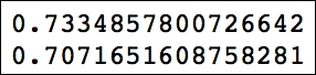
print(evaluator.evaluate(results, 
     {evaluator.metricName: 'areaUnderROC'}))
print(evaluator.evaluate(results, 
     {evaluator.metricName: 'areaUnderPR'}))

The preceding code will produce the following result:

As you can see, we got a slightly better result. What parameters does the best model have? The answer is a little bit convoluted, but here's how you can extract it:

results = [
    (
        [
            {key.name: paramValue} 
            for key, paramValue 
            in zip(
                params.keys(), 
                params.values())
        ], metric
    ) 
    for params, metric 
    in zip(
        cvModel.getEstimatorParamMaps(), 
        cvModel.avgMetrics
    )
]
sorted(results, 
       key=lambda el: el[1], 
       reverse=True)[0]

The preceding code produces the following output:

The TrainValidationSplit model, to select the best model, performs a random split of the input dataset (the training dataset) into two subsets: smaller training and validation subsets. The split is only performed once.

In this example, we will also use the ChiSqSelector to select only the top five features, thus limiting the complexity of our model:

selector = ft.ChiSqSelector(
    numTopFeatures=5, 
    featuresCol=featuresCreator.getOutputCol(), 
    outputCol='selectedFeatures',
    labelCol='INFANT_ALIVE_AT_REPORT'
)

The numTopFeatures specifies the number of features to return. We will put the selector after the featuresCreator, so we call the .getOutputCol() on the featuresCreator.

We covered creating the LogisticRegression and Pipeline earlier, so we will not explain how these are created again here:

logistic = cl.LogisticRegression(
    labelCol='INFANT_ALIVE_AT_REPORT',
    featuresCol='selectedFeatures'
)
pipeline = Pipeline(stages=[encoder, featuresCreator, selector])
data_transformer = pipeline.fit(births_train)

The TrainValidationSplit object gets created in the same fashion as the CrossValidator model:

tvs = tune.TrainValidationSplit(
    estimator=logistic, 
    estimatorParamMaps=grid, 
    evaluator=evaluator
)

As before, we fit our data to the model, and calculate the results:

tvsModel = tvs.fit(
    data_transformer 
        .transform(births_train)
)
data_train = data_transformer 
    .transform(births_test)
results = tvsModel.transform(data_train)
print(evaluator.evaluate(results, 
     {evaluator.metricName: 'areaUnderROC'}))
print(evaluator.evaluate(results, 
     {evaluator.metricName: 'areaUnderPR'}))

The preceding code prints out the following output:

Well, the model with less features certainly performed worse than the full model, but the difference was not that great. Ultimately, it is a performance trade-off between a more complex model and the less sophisticated one.