The main difference between using Jupyter and submitting jobs programmatically is the fact that you have to create your Spark context (and Hive, if you plan to use HiveQL), whereas when running Spark with Jupyter the contexts are automatically started for you.

In this section, we will develop a simple app that will use public data from Uber with trips made in the NYC area in June 2016; we downloaded the dataset from https://s3.amazonaws.com/nyc-tlc/trip+data/yellow_tripdata_2016-06.csv (beware as it is an almost 3GB file). The original dataset contains 11 million trips, but for our example we retrieved only 3.3 million and selected only a subset of all available columns.

So, let's get to it!

Things with Spark 2.0 have become slightly simpler than with previous versions when it comes to creating SparkContext. In fact, instead of creating a SparkContext explicitly, Spark currently uses SparkSession to expose higher-level functionality. Here's how you do it:

from pyspark.sql import SparkSession

spark = SparkSession 
        .builder 
        .appName('CalculatingGeoDistances') 
        .getOrCreate()

print('Session created')

The preceding code is all that you need!

In this example, we first create the SparkSession object and call its .builder internal class. The .appName(...) method allows us to give our application a name, and the .getOrCreate() method either creates or retrieves an already created SparkSession. It is a good convention to give your application a meaningful name as it helps to (1) find your application on a cluster and (2) creates less confusion for everyone.

Building your code in such a way so it can be reused later is always a good thing. The same can be done with Spark - you can modularize your methods and then reuse them at a later point. It also aids readability of your code and its maintainability.

In this example, we will build a module that would do some calculations on our dataset: It will compute the as-the-crow-flies distance (in miles) between the pickup and drop-off locations (using the Haversine formula), and also will convert the calculated distance from miles into kilometers.

So, first, we will build a module.

Structure of the module

We put the code for our extraneous methods inside the additionalCode folder.

Tip

Check out the GitHub repository for this book if you have not done so already https://github.com/drabastomek/learningPySpark/tree/master/Chapter11.

The tree for the folder looks as follows:

As you can see, it has a structure of a somewhat normal Python package: At the top we have the setup.py file so we can package up our module, and then inside we have our code.

The setup.py file in our case looks as follows:

from setuptools import setup

setup(
    name='PySparkUtilities',
    version='0.1dev',
    packages=['utilities', 'utilities/converters'],
    license='''
        Creative Commons 
        Attribution-Noncommercial-Share Alike license''',
    long_description='''
        An example of how to package code for PySpark'''
)

We will not delve into details here on the structure (which on its own is fairly self-explanatory): You can read more about how to define setup.py files for other projects here https://pythonhosted.org/an_example_pypi_project/setuptools.html.

The __init__.py file in the utilities folder has the following code:

from .geoCalc import geoCalc
__all__ = ['geoCalc','converters']

It effectively exposes the geoCalc.py and converters (more on these shortly).

from abc import ABCMeta, abstractmethod

class BaseConverter(metaclass=ABCMeta):
    @staticmethod
    @abstractmethod
    def convert(f, t):
        raise NotImplementedError

python setup.py bdist_egg

import utilities.geoCalc as geo
from utilities.converters import metricImperial

getDistance = func.udf(
    lambda lat1, long1, lat2, long2: 
        geo.calculateDistance(
            (lat1, long1),
            (lat2, long2)
        )
    )

convertMiles = func.udf(lambda m: 
    metricImperial.convert(str(m) + ' mile', 'km'))

uber = uber.withColumn(
    'miles', 
        getDistance(
            func.col('pickup_latitude'),
            func.col('pickup_longitude'), 
            func.col('dropoff_latitude'), 
            func.col('dropoff_longitude')
        )
    )

uber = uber.withColumn(
    'kilometers', 
    convertMiles(func.col('miles')))

In your CLI type the following (we assume you keep the structure of the folders unchanged from how it is structured on GitHub):

./launch_spark_submit.sh 
--master local[4] 
--py-files additionalCode/dist/PySparkUtilities-0.1.dev0-py3.5.egg 
calculatingGeoDistance.py

We owe you some explanation for the launch_spark_submit.sh shell script. In Bonus Chapter 1, Installing Spark, we configured our Spark instance to run Jupyter (by setting the PYSPARK_DRIVER_PYTHON system variable to jupyter). If you were to simply use spark-submit on a machine configured in such a way, you would most likely get some variation of the following error:

jupyter: 'calculatingGeoDistance.py' is not a Jupyter command

Thus, before running the spark-submit command we first have to unset the variable and then run the code. This would quickly become extremely tiring so we automated it with the launch_spark_submit.sh script:

#!/bin/bash

unset PYSPARK_DRIVER_PYTHON
spark-submit $*
export PYSPARK_DRIVER_PYTHON=jupyter

As you can see, this is nothing more than a wrapper around the spark-submit command.

If all goes well, you will see the following stream of consciousness appearing in your CLI:

There's a host of useful things that you can get from reading the output:

Once the job finishes, you will see something similar to the following:

From the preceding screenshot, we can read that the distances are reported correctly. You can also see that the Spark UI process has now been stopped and all the clean up jobs have been performed.

When you use the spark-submit command, Spark launches a local server that allows you to track the execution of the job. Here's what the window looks like:

At the top you can switch between the Jobs or Stages view; the Jobs view allows you to track the distinct jobs that are executed to complete the whole script, while the Stages view allows you to track all the stages that are executed.

You can also peak inside each stage execution profile and track each task execution by clicking on the link of the stage. In the following screenshot, you can see the execution profile for Stage 3 with four tasks running:

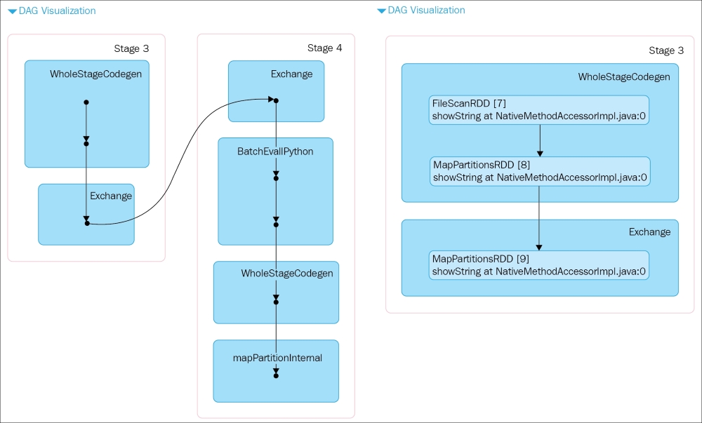
Inside a job or a stage, you can click on the DAG Visualization to see how your job or stage gets executed (the following chart on the left shows the Job view, while the one on the right shows the Stage view):