
Analytical queries that scan huge amounts of data were always problematic in a relational database. Nonclustered balanced tree indexes are efficient for transactional queries seeks; however, they rarely help with analytical queries. A great idea occurred nearly 30 years ago: why do we need to store data physically in the same way we work with it logically—row by row? Why don't we store it column by column and transform columns back to rows when we interact with the data? Microsoft was playing with this idea for a long time and finally implemented it in SQL Server.
Columnar storage was first added to SQL Server in version 2012. It included nonclustered columnstore indexes (NCCI) only. Clustered columnstore indexes (CCI) were added in version 2014. In this chapter, the readers revise the columnar storage and then explore huge improvements for columnstore indexes in SQL Server 2016: updatable nonclustered columnstore indexes, columnstore indexes on in-memory tables, and many other new features for operational analytics.
In the first section, you will learn about the SQL Server support for analytical queries without using the columnar storage. The next section of this chapter jumps directly to the columnar storage and explains the internals about it, with the main focus on columnar storage compression. In addition, the batch execution mode is introduced.
Then it is time to show columnar storage in action. The chapter starts with a section that introduces the nonclustered columnstore indexes. The demo code shows the compression you can get with this storage and also how to create a filtered nonclustered columnstore index.
The clustered columnstore indexes can have even better compression. You will learn how much these clustered and nonclustered columnstore indexes compress data and improve the performance of your queries. You can also combine columnar indexes with regular B-tree indexes. In addition, you will learn how to update data in a clustered columnstore index, especially how to insert new data efficiently. Finally, the chapter introduces the way to use columnar indexes together with regular B-tree indexes to implement a solution for operational analytics.
This chapter will cover the following points:
- Data compression in SQL Server
- Indexing for analytical queries
- T-SQL support for analytical queries
- Columnar storage basics
- Nonclustered columnstore indexes
- Using clustered columnstore indexes
- Creating regular B-tree indexes for tables with CCI
- Discovering support for primary and foreign keys for tables with CCI
- Discovering additional performance improvements with batch mode
- Columnstore indexes query performance
- Columnstore for real time operational analytics
- Data loading for columnstore indexes
Supporting analytical applications in SQL Server differs quite a lot from supporting transactional applications. The typical schema for reporting queries is the star schema. In a star schema, there is one central table called fact table and multiple surrounding tables called dimensions. The fact table is always on the many side of every relationship with every dimension. The database that supports analytical queries and uses the star schema design is called Data Warehouse (DW). Dealing with data warehousing design in detail is out of the scope of this book. Nevertheless, there is a lot of literature available. For a quick start, you can read the data warehouse concepts MSDN blog at https://blogs.msdn.microsoft.com/syedab/2010/06/01/data-warehouse-concepts/. The WideWorldImportersDW demo database implements multiple star schemas. The following screenshot shows a subset of tables from this database that supports analytical queries for sales:

Figure 10-1: Sales Star schema
Typical analytical queries require huge amounts of data, for example, sales data for two years, which is then aggregated. Therefore, index seeks are quite rare. Most of the times, you need to optimize the number of IO reads using different techniques than you would use in a transactional environment, where you have mostly selective queries that benefit a lot from index seeks. Columnstore indexes are the latest and probably the most important optimization for analytical queries in SQL Server. However, before going to the columnar storage, you should be familiar with other techniques and possibilities for optimizing data warehousing scenarios. All you will learn about in this section will help you understand the need for and the implementation of columnstore indexes. You will learn about the following:
- Join types
- Bitmap filtered hash joins
- B-tree indexes for analytical queries
- Filtered nonclustered indexes
- Table partitioning
- Indexed views
- Row compression
- Page compression
- Appropriate query techniques
SQL Server executes a query by a set of physical operators. Because these operators iterate through rowsets, they are also called iterators. There are different join operators, because when performing joins, SQL Server uses different algorithms. SQL Server supports three basic algorithms: nested loops joins, merge joins, and hash joins. A hash join can be further optimized by using bitmap filtering; a bitmap filtered hash join could be treated as the fourth algorithm or as an enhancement of the third, the hash algorithm. The last one, the bitmap filtered hash join, is an example of SQL Server's optimization for analytical queries.
The nested loops algorithm is a very simple and, in many cases, efficient algorithm. SQL Server uses one table for the outer loop, typically the table with fewer rows. For each row in this outer input, SQL Server seeks matching rows in the second table, which is the inner table. SQL Server uses the join condition to find the matching rows. The join can be a non-equijoin, meaning that the equality operator does not need to be part of the join predicate. If the inner table has no supporting index to perform seeks, then SQL Server scans the inner input for each row of the outer input. This is not an efficient scenario. A nested loops join is efficient when SQL Server can perform an index seek in the inner input.
Merge join is a very efficient join algorithm. However, it has its own limitations. It needs at least one equijoin predicate and sorted inputs from both sides. This means that the merge join should be supported by indexes on both tables involved in the join. In addition, if one input is much smaller than another, then the nested loops join could be more efficient than a merge join.
In a one-to-one or one-to-many scenario, the merge join scans both inputs only once. It starts by finding the first rows on both sides. If the end of the input is not reached, the merge join checks the join predicate to determine whether the rows match. If the rows match, they are added to the output. Then the algorithm checks the next rows from the other side and adds them to the output until they match the predicate. If the rows from the inputs do not match, then the algorithm reads the next row from the side with the lower value from the other side. It reads from this side and compares the row to the row from the other side until the value is bigger than the value from the other side. Then it continues reading from the other side, and so on. In a many-to-many scenario, the merge join algorithm uses a worktable to put the rows from one input side aside for reusage when duplicate matching rows from the other input exist.
If none of the inputs is supported by an index and an equijoin predicate is used, then the hash join algorithm might be the most efficient one. It uses a searching structure named hash table. This is not a searching structure you can build like a balanced tree used for indexes. SQL Server builds the hash table internally. It uses a hash function to split the rows from the smaller input into buckets. This is the build phase. SQL Server uses the smaller input for building the hash table because SQL Server wants to keep the hash table in memory. If it needs to get spilled out to tempdb on disk, then the algorithm might become much slower. The hash function creates buckets of approximately equal size.
After the hash table is built, SQL Server applies the hash function on each of the rows from the other input. It checks to see which bucket the row fits. Then it scans through all rows from the bucket. This phase is called the probe phase.
A hash join is a kind of compromise between creating a full balanced tree index and then using a different join algorithm and performing a full scan of one side input for each row of the other input. At least in the first phase, a seek of the appropriate bucket is used. You might think that the hash join algorithm is not efficient. It is true that in a single-thread mode, it is usually slower than merge and nested loops join algorithms that are supported by existing indexes. However, SQL Server can split rows from the probe input in advance. It can push the filtering of the rows that are candidates for a match with a specific hash bucket down to the storage engine. This kind of optimization of a hash join is called a bitmap filtered hash join. It is typically used in a data warehousing scenario, where you can have large inputs for a query, which might not be supported by indexes. In addition, SQL Server can parallelize query execution and perform partial joins in multiple threads. In data warehousing scenarios, it is not uncommon to have only a few concurrent users, so SQL Server can execute a query in parallel. Although a regular hash join can be executed in parallel as well, the bitmap filtered hash join is even more efficient because SQL Server can use bitmaps for early elimination of rows not used in the join from the bigger table involved in the join.
In the bitmap filtered hash join, SQL Server first creates a bitmap representation of a set of values from a dimension table to prefilter rows to join from a fact table. A bitmap filter is a bit array of m bits. Initially, all bits are set to 0. Then SQL Server defines k different hash functions. Each one maps some set element to one of the m positions with a uniform random distribution. The number of hash functions k must be smaller than the number of bits in array m. SQL Server feeds each of the k hash functions to get k array positions with values from dimension keys. It set the bits at all these positions to 1. Then SQL Server tests the foreign keys from the fact table. To test whether any element is in the set, SQL Server feeds it to each of the k hash functions to get k array positions. If any of the bits at these positions are 0, the element is not in the set. If all are 1, then either the element is in the set, or the bits have been set to 1 during the insertion of other elements. The following diagram shows the bitmap filtering process:

Figure 10.2: Bitmap filtering
In the preceding diagram, the length m of the bit array is 16. The number k of hash functions is 3. When feeding the hash functions with the values from the set {a, b, c}, which represents dimension keys, SQL Server sets bits at positions 2, 4, 5, 6, 11, 12, and 14 to 1 (starting numbering positions with 1). Then SQL Server feeds the same hash functions with the value w from the smaller set at the bottom {w}, which represents a key from a fact table. The functions would set bits at positions 4, 9, and 12 to 1. However, the bit at position 9 is set to 0. Therefore, the value w is not in the set {a, b, c}.
Bitmap filters return so-called false positives. They never return false negatives. This means that when you declare that a probe value might be in the set, you still need to scan the set and compare it to each value from the set. The more false positive values a bitmap filter returns, the less efficient it is. Note that if the values in the probe side in the fact table are sorted, it will be quite easy to avoid the majority of false positives.
The following query reads the data from the tables introduced earlier in this section and implements star schema optimized bitmap filtered hash joins:
USE WideWorldImportersDW;
SELECT cu.[Customer Key] AS CustomerKey, cu.Customer,
  ci.[City Key] AS CityKey, ci.City,
  ci.[State Province] AS StateProvince, ci.[Sales Territory] AS SalesTeritory,
  d.Date, d.[Calendar Month Label] AS CalendarMonth,
  d.[Calendar Year] AS CalendarYear,
  s.[Stock Item Key] AS StockItemKey, s.[Stock Item] AS Product, s.Color,
  e.[Employee Key] AS EmployeeKey, e.Employee,
  f.Quantity, f.[Total Excluding Tax] AS TotalAmount, f.Profit
FROM Fact.Sale AS f
  INNER JOIN Dimension.Customer AS cu
    ON f.[Customer Key] = cu.[Customer Key]
  INNER JOIN Dimension.City AS ci
    ON f.[City Key] = ci.[City Key]
  INNER JOIN Dimension.[Stock Item] AS s
    ON f.[Stock Item Key] = s.[Stock Item Key]
  INNER JOIN Dimension.Employee AS e
    ON f.[Salesperson Key] = e.[Employee Key]
  INNER JOIN Dimension.Date AS d
    ON f.[Delivery Date Key] = d.Date;
The following diagram shows a part of the execution plan. You can see the Bitmap Create operator that is fed with values from the dimension date table. The filtering of the fact table is done in the Hash Match operator:

Figure 10-3: Bitmap Create operator in the execution plan
SQL Server stores a table as a heap or as a balanced tree (B-tree). If you create a clustered index, a table is stored as a B-tree. As a general best practice, you should store every table with a clustered index because storing a table as a B-tree has many advantages, as listed here:
- You can control table fragmentation with the
ALTER INDEXcommand using theREBUILDorREORGANIZEoption. - A clustered index is useful for range queries because the data is logically sorted on the key.
- You can move a table to another filegroup by recreating the clustered index on a different filegroup. You do not have to drop the table as you would to move a heap.
- A clustering key is a part of all nonclustered indexes. If a table is stored as a heap, then the row identifier is stored in nonclustered indexes instead. A short integer-clustering key is shorter than a row identifier, thus making nonclustered indexes more efficient.
- You cannot refer to a row identifier in queries, but clustering keys are often part of queries. This raises the probability for covered queries. Covered queries are queries that read all data from one or more nonclustered indexes without going to the base table. This means that there are fewer reads and less disk IO.
Clustered indexes are particularly efficient when the clustering key is short. Creating a clustering index with a long key makes all nonclustered indexes less efficient. In addition, the clustering key should be unique. If it is not unique, SQL Server makes it unique by adding a 4-byte sequential number called uniquifier to duplicate keys. Uniquifier becomes a part of the clustering key, which is duplicated in every nonclustered index. This makes keys longer and all indexes less efficient. Clustering keys could be useful if they are ever-increasing. With ever-increasing keys, minimally logged bulk inserts are possible even if a table already contains data, as long as the table does not have additional nonclustered indexes.
Data warehouse surrogate keys are often ideal for clustered indexes. Because you are the one who defines them, you can define them as efficiently as possible. Use integers with autonumbering options. The primary key constraint creates a clustered index by default. In addition, clustered indexes can be very useful for partial scans. Remember that analytical queries typically involve a lot of data and, therefore, don't use seeks a lot. However, instead of scanning the whole table, you can find the first value with a seek and then perform a partial scan until you reach the last value needed for the query result. Many times, analytical queries use date filters; therefore, a clustering key over a date column might be ideal for such queries.
You need to decide whether to optimize your tables for data load or for querying. However, with partitioning, you can get both—efficient data load without a clustered key on an ever-increasing column, and more efficient queries with partial scans. In order to show the efficiency of partial scans, let's first create a new table organized as a heap with the following query:
SELECT 1 * 1000000 + f.[Sale Key] AS SaleKey,
  cu.[Customer Key] AS CustomerKey, cu.Customer,
  ci.[City Key] AS CityKey, ci.City,
  f.[Delivery Date Key] AS DateKey,
  s.[Stock Item Key] AS StockItemKey, s.[Stock Item] AS Product,
  f.Quantity, f.[Total Excluding Tax] AS TotalAmount, f.Profit
INTO dbo.FactTest
FROM Fact.Sale AS f
  INNER JOIN Dimension.Customer AS cu
    ON f.[Customer Key] = cu.[Customer Key]
  INNER JOIN Dimension.City AS ci
    ON f.[City Key] = ci.[City Key]
  INNER JOIN Dimension.[Stock Item] AS s
    ON f.[Stock Item Key] = s.[Stock Item Key]
  INNER JOIN Dimension.Date AS d
    ON f.[Delivery Date Key] = d.Date;
Now you can turn the STATISTICS IO on to show the number of logical reads in the following two queries:
SET STATISTICS IO ON;
-- All rows
SELECT *
FROM dbo.FactTest;
-- Date range
SELECT *
FROM dbo.FactTest
WHERE DateKey BETWEEN '20130201' AND '20130331';
SET STATISTICS IO OFF;
SQL Server used a Table Scan operator for executing both queries. For both of them, even though the second one used a filter on the delivery date column, SQL Server performed 5,893 logical IOs.
Now let's create a clustered index in the delivery date column:
CREATE CLUSTERED INDEX CL_FactTest_DateKey
ON dbo.FactTest(DateKey);
GO
If you execute the aforementioned same two queries, you get around 6,091 reads and the Clustered Index Scan operator for the first query, and 253 logical reads for the second query, with Clustered Index Seek operator that finds the first value needed for the query and performs a partial scan after.
Loading even very large fact tables is not a problem if you can perform incremental loads. However, this means that data in the source should never be updated or deleted; data should only be inserted. This is rarely the case with LOB applications. In addition, even if you have the possibility of performing an incremental load, you should have a parameterized ETL procedure in place so you can reload portions of data loaded already in earlier loads. There is always a possibility that something might go wrong in the source system, which means that you will have to reload historical data. This reloading will require you to delete part of the data from your data warehouse.
Deleting large portions of fact tables might consume too much time unless you perform a minimally logged deletion. A minimally logged deletion operation can be done using the TRUNCATE TABLE command; however, this command deletes all the data from a table, and deleting all the data is usually not acceptable. More commonly, you need to delete only portions of the data.
Inserting huge amounts of data could consume too much time as well. You can do a minimally logged insert, but as you already know, minimally logged inserts have some limitations. Among other limitations, a table must either be empty, have no indexes, or use a clustered index only on an ever-increasing (or ever-decreasing) key so that all inserts occur on one end of the index.
You can resolve all of these problems by partitioning a table. You can even achieve better query performance using a partitioned table because you can create partitions in different filegroups on different drives, thus parallelizing reads. In addition, SQL Server query optimizer can do early partition elimination, so SQL Server does not even touch a partition with data excluded from the result set of a query. You can also perform maintenance procedures on a subset of filegroups and thus on a subset of partitions only. That way, you can also speed up regular maintenance tasks. Altogether, partitions have many benefits.
Although you can partition a table on any attribute, partitioning over dates is most common in data warehousing scenarios. You can use any time interval for a partition. Depending on your needs, the interval could be a day, a month, a year, or any other interval.
In addition to partitioning tables, you can also partition indexes. If indexes are partitioned in the same way as the base tables, they are called aligned indexes. Partitioned table and index concepts include the following:
- Partition function: This is an object that maps rows to partitions by using values from specific columns. The columns used for the function are called partitioning columns. A partition function performs logical mapping.
- Partition scheme: A partition scheme maps partitions to filegroups. A partition scheme performs physical mapping.
- Aligned index: This is an index built on the same partition scheme as its base table. If all indexes are aligned with their base table, switching a partition is a metadata operation only, so it is very fast. Columnstore indexes have to be aligned with their base tables. Nonaligned indexes are, of course, indexes that are partitioned differently than their base tables.
- Partition switching: This is a process that switches a block of data from one table or partition to another table or partition. You switch the data by using the
ALTER TABLE T-SQLcommand. You can perform the following types of switches:- Reassign all data from a nonpartitioned table to an empty existing partition of a partitioned table
- Switch a partition of a one-partitioned table to a partition of another partitioned table
- Reassign all data from a partition of a partitioned table to an existing empty nonpartitioned table
- Partition elimination: This is a query optimizer process in which SQL Server accesses only those partitions needed to satisfy query filters.
For more information about table and index partitioning, refer to the MSDN Partitioned Tables and Indexes article at https://msdn.microsoft.com/en-us/library/ms190787.aspx.
As mentioned, data warehouse queries typically involve large scans of data and aggregation. Very selective seeks are not common for reports from a DW. Therefore, nonclustered indexes generally don't help DW queries much. However, this does not mean that you shouldn't create any nonclustered indexes in your DW.
An attribute of a dimension is not a good candidate for a nonclustered index key. Attributes are used for pivoting and typically contain only a few distinct values. Therefore, queries that filter based on attribute values are usually not very selective. Nonclustered indexes on dimension attributes are not a good practice.
DW reports can be parameterized. For example, a DW report could show sales for all customers or for only a single customer, based perhaps on parameter selection by an end user. For a single-customer report, the user would choose the customer by selecting that customer's name. Customer names are selective, meaning that you retrieve only a small number of rows when you filter by customer name. Company names, for example, are typically unique, so by filtering by a company name, you typically retrieve a single row. For reports like these, having a nonclustered index on a name column or columns could lead to better performance.
You can create a filtered nonclustered index. A filtered index spans a subset of column values only and thus applies to a subset of table rows. Filtered nonclustered indexes are useful when some values in a column occur rarely, whereas other values occur frequently. In such cases, you would create a filtered index over the rare values only. SQL Server uses this index for seeks of rare values but performs scans for frequent values. Filtered nonclustered indexes can be useful not only for name columns and member properties but also for attributes of a dimension, and even foreign keys of a fact table. For example, in our demo fact table, the customer with ID equal to 378 has only 242 rows. You can execute the following code to show that even if you select data for this customer only, SQL Server performs a full scan:
SET STATISTICS IO ON;
-- All rows
SELECT *
FROM dbo.FactTest;
-- Customer 378 only
SELECT *
FROM dbo.FactTest
WHERE CustomerKey = 378;
SET STATISTICS IO OFF;
Both queries needed 6,091 logical reads. Now you can add a filtered nonclustered index to the table:
CREATE INDEX NCLF_FactTest_C378
 ON dbo.FactTest(CustomerKey)
 WHERE CustomerKey = 378;
GO
If you execute the same two queries again, you get much less IO for the second query. It needed 752 logical reads in my case and used the Index Seek and Key Lookup operators.
You can drop the filtered index when you don't need it anymore with the following code:
DROP INDEX NCLF_FactTest_C378
 ON dbo.FactTest;
GO
You can optimize queries that aggregate data and perform multiple joins by permanently storing the aggregated and joined data. For example, you could create a new table with joined and aggregated data and then maintain that table during your ETL process.
However, creating additional tables for joined and aggregated data is not best practice because using these tables means you have to change queries used in your reports. Fortunately, there is another option for storing joined and aggregated tables. You can create a view with a query that joins and aggregates data. Then you can create a clustered index on the view to get an indexed view. With indexing, you are materializing a view; you are storing physically the data the view is returning when you query it. In the Enterprise or Developer Edition of SQL Server, SQL Server Query Optimizer uses the indexed view automatically—without changing the query. SQL Server also maintains indexed views automatically. However, to speed up data loads, you can drop or disable the index before load and then recreate or rebuild it after the load.
For example, note the following query that aggregates the data from the test fact table:
SET STATISTICS IO ON;
SELECT StockItemKey,
 SUM(TotalAmount) AS Sales,
 COUNT_BIG(*) AS NumberOfRows
FROM dbo.FactTest
GROUP BY StockItemKey;
SET STATISTICS IO OFF;
In my case, this query used 6,685 logical IOs. It used the clustered Index scan operator on the fact table to retrieve the whole dataset. Now let's create a view with the same query used for the definition:
CREATE VIEW dbo.SalesByProduct
WITH SCHEMABINDING AS
SELECT StockItemKey,
 SUM(TotalAmount) AS Sales,
 COUNT_BIG(*) AS NumberOfRows
FROM dbo.FactTest
GROUP BY StockItemKey;
GO
Indexed views have many limitations. One of them is that they have to be created with the SCHEMABINDING option if you want to index them, as you can see in the previous code. Now let's index the view:
CREATE UNIQUE CLUSTERED INDEX CLU_SalesByProduct
 ON dbo.SalesByProduct (StockItemKey);
GO
Try to execute the last query before creating the view again. Make sure you notice that the query refers to the base table and not the view. This time, the query needed only four logical reads. If you check the execution plan, you should see that SQL Server used the Clustered Index Scan operator on the indexed view. If your indexed view was not used automatically, please check which edition of SQL Server you use. When you finish with testing, you can drop the view with the following code:
DROP VIEW dbo.SalesByProduct;
GO
SQL Server supports data compression. Data compression reduces the size of the database, which helps improve query performance because queries on compressed data read fewer pages from disk and thus use less IO. However, data compression requires extra CPU resources for updates, because data must be decompressed before and compressed after the update. Data compression is therefore suitable for data warehousing scenarios in which data is mostly read and only occasionally updated.
SQL Server supports three compression implementations:
- Row compression: Row compression reduces metadata overhead by storing fixed data type columns in a variable-length format. This includes strings and numeric data. Row compression has only a small impact on CPU resources and is often appropriate for OLTP applications as well.
- Page compression: Page compression includes row compression, but also adds prefix and dictionary compressions. Prefix compression stores repeated prefixes of values from a single column in a special compression information structure that immediately follows the page header, replacing the repeated prefix values with a reference to the corresponding prefix. Dictionary compression stores repeated values anywhere in a page in the compression information area. Dictionary compression is not restricted to a single column.
- Unicode compression: In SQL Server, Unicode characters occupy an average of two bytes. Unicode compression substitutes single-byte storage for Unicode characters that don't truly require two bytes. Depending on collation, Unicode compression can save up to 50 per cent of the space otherwise required for Unicode strings. Unicode compression is very cheap and is applied automatically when you apply either row or page compression.
You can gain quite a lot from data compression in a data warehouse. Foreign keys are often repeated many times in a fact table. Large dimensions that have Unicode strings in name columns, member properties, and attributes can benefit from Unicode compression.
The following diagram explains dictionary compression:
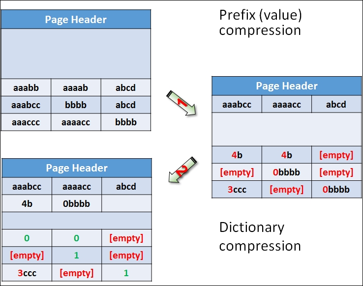
Figure 10.4: Dictionary compression
As you can see from the diagram, the dictionary compression (corresponding to the first arrow) starts with prefix compression. In the compression information space on the page right after the page header, you can find stored prefixes for each column. If you look at the top left cell, the value in the first row, first column, is aaabb. The next value in this column is aaabcc. A prefix value aaabcc is stored for this column in the first column of the row for the prefix compression information. Instead of the original value in the top left cell, a value 4b is stored. This means use four characters from the prefix for this column and add the letter b to get back the original value. The value in the second row for the first column is empty because the prefix for this column is equal to the whole original value in that position. The value in the last row for the first column after the prefix compression is 3ccc, meaning that in order to get the original value, you need to take the first three characters from the column prefix and add a string ccc, thus getting the value aaaccc, which is, of course, equal to the original value. Check also the prefix compression for other two columns.
After the prefix compression, dictionary compression is applied (corresponding to the second arrow in the Figure 10.4). It checks all strings across all columns to find common substrings. For example, the value in the first two columns of the first row after the prefix compression was applied is 4b. SQL Server stores this value in the dictionary compression information area as the first value in this area, with index 0. In the cells, it stores just the index value 0 instead of the value 4b. The same happens for the value 0bbbb, which you can find in the second row, second column, and third row, third column, after prefix compression is applied. This value is stored in the dictionary compression information area in the second position with index 1; in the cells, the value 1 is left.
You might wonder why prefix compression is needed. For strings, a prefix is just another substring, so the dictionary compression could cover the prefixes as well. However, prefix compression can work on nonstring data types as well. For example, instead of storing integers 900, 901, 902, 903, and 904 in the original data, you can store a prefix 900 and leave values 0, 1, 2, 3, and 4 in the original cells.
Now it's time to test SQL Server compression. First of all, let's check the space occupied by the test fact table:
EXEC sys.sp_spaceused N'dbo.FactTest', @updateusage = N'TRUE';
GO
The result is as follows:
Name          rows    reserved  data      index_size  unused
------------  ------  --------  --------  ----------  ------
dbo.FactTest  227981  49672 KB  48528 KB      200 KB  944 KB
The following code enables row compression on the table and checks the space used again:
ALTER TABLE dbo.FactTest
 REBUILD WITH (DATA_COMPRESSION = ROW);
EXEC sys.sp_spaceused N'dbo.FactTest', @updateusage = N'TRUE';
This time the result is as follows:
Name          rows    reserved  data      index_size  unused
------------  ------  --------  --------  ----------  ------
dbo.FactTest  227981  25864 KB  24944 KB       80 KB  840 KB
You can see that a lot of space was saved. Let's also check the page compression:
ALTER TABLE dbo.FactTest
 REBUILD WITH (DATA_COMPRESSION = PAGE);
EXEC sys.sp_spaceused N'dbo.FactTest', @updateusage = N'TRUE';
Now the table occupies even less space, as the following result shows:
Name          rows    reserved  data      index_size  unused
------------  ------  --------  --------  ----------  ------
dbo.FactTest  227981  18888 KB  18048 KB       80 KB  760 KB
If these space savings are impressive for you, wait for the columnstore compression! Anyway, before continuing, you can remove the compression from the test fact table with the following code:
ALTER TABLE dbo.FactTest
 REBUILD WITH (DATA_COMPRESSION = NONE);
Before continuing with other SQL Server features that support analytics, I want to explain another compression algorithm because this algorithm is also used in columnstore compression. The algorithm is called LZ77 compression. It was published by Abraham Lempel and Jacob Ziv in 1977; the name of the algorithm comes from the first letters of the author's last names plus the publishing year. The algorithm uses sliding window dictionary encoding, meaning it encodes chunks of an input stream with dictionary encoding. The following are the steps of the process:
- Set the coding position to the beginning of the input stream.
- Find the longest match in the window for the look ahead buffer.
- If a match is found, output the pointer P and move the coding position (and the window) L bytes forward.
- If a match is not found, output a null pointer and the first byte in the look ahead buffer and move the coding position (and the window) one byte forward.
- If the look ahead buffer is not empty, return to step 2.
The following figure explains this process in an example:

Figure 10.5: LZ77 compression
The input stream chunk that is compressed in the figure is AABCBBABC:
- The algorithm starts encoding from the beginning of the window of the input stream. It stores the first byte (the A value) in the result, together with the pointer (0,0), meaning this is a new value in this chunk.
- The second byte is equal to the first one. The algorithm stores just the pointer (1,1) to the output. This means that in order to recreate this value, you need to move one byte back and read one byte.
- The next two values, B and C, are new and are stored to the output together with the pointer (0,0).
- Then the B value repeats. Therefore, the pointer (2,1) is stored, meaning that in order to find this value, you need to move two bytes back and read one byte.
- Then the B value repeats again. This time, you need to move one byte back and read one byte to get the value, so the value is replaced with the pointer (1,1). You can see that when you move back and read the value, you get another pointer. You can have a chain of pointers.
- Finally, the substring ABC is found in the stream. This substring can be also found in the positions 2-4. Therefore, in order to recreate the substring, you need to move five bytes back and read three bytes, and the pointer (5,3) is stored in the compressed output.
Before finishing this section, I also need to mention that no join or compression algorithm, or any other feature that SQL Server offers can help you if you write inefficient queries. A good example of a typical DW query is one that involves running totals. You can use non-equi self joins for such queries, which is a very good example of an inefficient query. The following code calculates the running total for the profit ordered over the sale key with a self join. The code also measures IO and time needed for executing the query. Note that the query uses a CTE first to select only 12,000 rows from the fact table. A non-equi self join is a quadratic algorithm; with double the amount of the rows, the time needed increases four times. You can play with different amount of rows to prove that:
SET STATISTICS IO ON;
SET STATISTICS TIME ON;
WITH SalesCTE AS
(
SELECT [Sale Key] AS SaleKey, Profit
FROM Fact.Sale
WHERE [Sale Key] <= 12000
)
SELECT S1.SaleKey,
 MIN(S1.Profit) AS CurrentProfit,
 SUM(S2.Profit) AS RunningTotal
FROM SalesCTE AS S1
 INNER JOIN SalesCTE AS S2
  ON S1.SaleKey >= S2.SaleKey
GROUP BY S1.SaleKey
ORDER BY S1.SaleKey;
SET STATISTICS IO OFF;
SET STATISTICS TIME OFF;
With 12,000 rows, the query needed 817,584 logical reads in a worktable, which is a temporary representation of the test fact table on the right side of the self join, and on the top of it, more than 3,000 logical reads for the left representation of the fact table. On my computer, it took more than 12 seconds (elapsed time) to execute this query, with more than 72 seconds of CPU time, as the query was executed with a parallel execution plan. With 6,000 rows, the query would need approximately four times less IO and time.
You can calculate running totals very efficiently with window aggregate functions. The following example shows the query rewritten. The new query uses the window aggregate functions:
SET STATISTICS IO ON;
SET STATISTICS TIME ON;
WITH SalesCTE AS
(
SELECT [Sale Key] AS SaleKey, Profit
FROM Fact.Sale
WHERE [Sale Key] <= 12000
)
SELECT SaleKey,
 Profit AS CurrentProfit,
 SUM(Profit)
   OVER(ORDER BY SaleKey
        ROWS BETWEEN UNBOUNDED PRECEDING
                 AND CURRENT ROW) AS RunningTotal
FROM SalesCTE
ORDER BY SaleKey;
SET STATISTICS IO OFF;
SET STATISTICS TIME OFF;
This time, the query used 331 reads in the fact table, 0 (zero) reads in the worktable, 0.15 second elapsed time, and 0.02 second CPU time. SQL Server didn't even bother to find a parallel plan.