Chapter 8: Beginning Advanced Analytics

In Chapter 7, Extracting Value, we developed our skills for analyzing your data and producing a report to consume your insights. In this chapter, we will extend our capabilities to complete a spatial analysis and start a Machine Learning (ML) project.

Using the spatial capabilities of Alteryx, we will learn about how we can generate spatial information in our dataset and use that spatial information to find the geographic relationships that are present.

Next, we will investigate the different options for building an ML project. We will investigate three levels of control for deploying an ML model built from a fully automated process to get complete control of all processes.

These topics will cover how to gain analytic insights directly from an Alteryx workflow. We will also see how we can leverage the Alteryx Server gallery to provide automated insights and extract these insights in an automated manner.

We will cover the following topics in this chapter:

• Implementing spatial analytics with Alteryx
• Beginning the ML process in Alteryx

Technical requirements

In this chapter, you will need access to Alteryx Designer with the predictive tools installed for creating workflows. The install process is discussed in the Building workflows with R-based predictive tools section later in the chapter. The predictive tools require a separate Alteryx install package but do not have any additional licensing cost associated with them.

The Using the Intelligence Suite section requires the Intelligence Suite add-on to the designer package. This add-on is separately licensed to the main Alteryx Designer package and therefore, to complete that section of the exercises, you will require access to that license. The example workflows can be found in the book's GitHub repository here: https://github.com/PacktPublishing/Data-Engineering-with-Alteryx/tree/main/Chapter%2008.

Finally, the datasets we will be using for this chapter are all part of the Alteryx install. You can find them in the Alteryx sample data folder. By default, it is located at C:Program FilesAlteryxSamplesdata.

The other way to find the folder location is by navigating to the Help option in the menu bar of Alteryx and clicking on Sample Datasets, as you can see in the following screenshot:

Figure 8.1 – Location of the sample data from the Help menu

Using the sample datasets, let's learn how to perform spatial analytics with Alteryx.

Implementing spatial analytics with Alteryx

Spatial analysis is about taking the geographic location of something and finding patterns related to its geographic location. In Alteryx, you can perform a spatial analysis by leveraging the Spatial Tool Pallet and creating a spatial object. To achieve spatial analysis using spatial tools, you need to create a spatial object. The essential spatial object type is a spatial point.

Creating a spatial point

The primary way of creating a spatial point is by using the Create Points tool. This tool will take two coordinate fields to assign one to the X coordinate point and the other to the Y coordinate point. For example, the following screenshot shows the configuration:

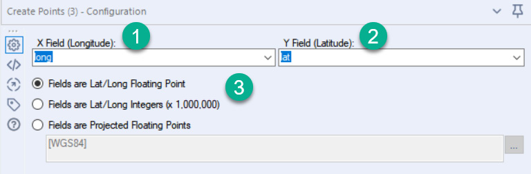
Figure 8.2 – Configuration of the Create Points tool

We will be using the HousingPricesTestData.yxdb dataset, which contains long and lat fields. The long field contains longitude information (step 1 in the screenshot), while the lat field holds the latitude information (step 2 in the screenshot). Finally, you can change the projection type. We have decimal values for the latitude and longitude for our data, hence the first option (Fields are Lat/Long Floating Point). The other options are for when your latitude and longitude are integers or using a different projection system. The different projection systems are developed and maintained by external standards organizations, but are available in the Fields are Projected Floating Points menu.

The resulting output from the Create Points tool is a new spatial object field. This field appears in green text in the Results window with an identifier of the spatial object type. This is highlighted in the following screenshot with a box:

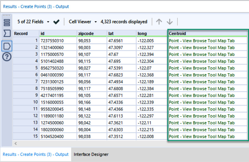
Figure 8.3 – Selected output from the Create Points tool in the Results window

You can see that each record in the image has Point – View Browse Tool Map Tab. For example, when you display the spatial object in the Browse tool, you see the points on a map, as seen in the following screenshot:

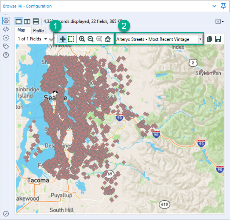
Figure 8.4 – Browse tool map tab for the spatial points created

When viewing the Map tab in the Browse tool, you can navigate the map using the zoom and selection buttons highlighted in box 1. Additionally, you can assign what base map you wish to view. The default configuration for Alteryx is to display no base map. By selecting the dropdown in box 2, you can set one of the other base map options. Any map with Most Recent Vintage appended to the map name will query the Alteryx map provider, MapBox, for any map image changes. All other map options will use a locally cached version of the base map you have selected.

Geocoding addresses to make spatial points

If you have addresses in your dataset but not the latitude or longitude coordinates, you cannot map the location using only that information. To create a spatial object, you need to geocode the records first. This is where address records are converted into latitude and longitude to create a spatial object. For example, if you have the Alteryx Location Insights dataset (which requires an additional add-on license), you can use the macro provided to cleanse and standardize addresses from the United States and Canada. Then you can geocode using the tools provided from that dataset.

If you don't have the Location Insights dataset, you can use one of the geocoding APIs available. One option is to use the Google Maps API. Because it is a commonly used method, the community has created macros that call this API, which are available on the Alteryx Community gallery (https://community.alteryx.com/gallery). In addition, Alteryx ACE James Dunkerley has released an excellent macro that you can download from the gallery (https://community.alteryx.com/t5/user/viewprofilepage/user-id/3554).

When using this macro, you need to provide two fields, as seen in the following screenshot:

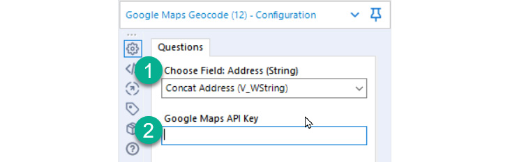
Figure 8.5 – The configuration for the Google Maps Geocode macro

When you configure the Google Maps Geocode macro, you need to provide two pieces of information:

1. The location you want to geocode: This location can be a building name, business name, or address. Essentially, you can geocode anything you might search for in Google Maps with this tool.
2. An API key for Google Maps: The API key needs to have the permissions for the Geocoding API. The information on how to use the API can be found in the Google Maps API documentation (https://developers.google.com/maps/documentation/geocoding/overview), including how to configure and create the API key.

With these two fields populated, you can query the API and return a geocoded output with the complete address information as well as lat and long fields for use with the Create Points tool.

Generating trade areas for analysis

Once we have a spatial point, we can perform additional analytics and find the relationships between different spatial objects. When working with spatial analysis, you often have areas of influence for individual points. For example, if you have a retail store, you would expect most of your customers to be from a radius around the store; this area is called a trade area. The tool is found in the Spatial tab of the tool pallet and the icon is shown in Figure 8.6:

Figure 8.6 – The Trade Area icon from the Spatial tab of the tool pallet

You create a trade area around a spatial point with the Trade Area tool. There are three highlighted parts in the following screenshot that you need to configure:

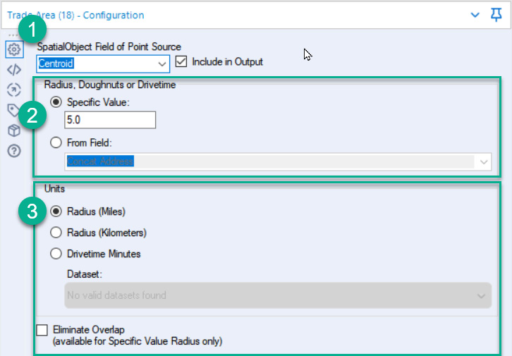
Figure 8.7 – Configuration of the Trade Area tool

When you configure the trade area, you will follow these steps:

1. Choose the spatial object you want a trade area around.
2. Define the size of the trade area you want. This trade area can either be a fixed value or customized from a field in your data. If you use a specific value, you can enter a comma-separated list and create a trade area for each value. When making a trade area, the first value you enter will be placed on your view first, with each following trade area stacked one on top of the other. So, if you put the largest trade area at the end, that will be the only area you see.
3. Finally, you can define the units for the trade area from the choices of Miles, Kilometers, or, if you have the Location Insights dataset, Drivetime Minutes.

Once you create the trade area, you will find other relationships in the geographic information in your data.

Combining data streams with spatial information

We can merge the multiple datasets based on their spatial features with the trade area created and the addresses geocoded. Two tools can match data streams together with their spatial information, the Spatial Match tool, and the Find Nearest tool.

We configure the spatial joining tools similarly. There is a target input and a universe input on the input side. The target is the dataset you are interested in keeping and establishing the relationship with. Only records from the target input will be sent to the output. The universe input is the records you want to identify as spatially close to your targets.

On the output side, both outputs are records from the target input. The match output is all the target records that have a matching record from the universe; this output will also include the fields from the matching universe record. The unmatched output is any target records that do not match the universe.

The difference between the spatial match and the Find Nearest tool defines a matching record, which is selected from a dropdown in the tool's configuration. The spatial match requires the spatial objects to overlap based on the intersection configuration. There are seven different intersection types:

• Where Target Intersects Universe: This match is when any part of the target overlaps with the universe.
• Where Target Contains Universe: This match requires that the entirety of the universe object is inside the target object.
• Where Target Is Within Universe: This is the reverse of the Where Target Touches Universe option and means the entirety of the target object is contained inside the universe object.
• Where Target Touches Universe: This match is where an edge, or boundary, of the target and universe objects share an exact location. It also requires that neither object has the same internal space.
• Where Target Touches or Intersects Universe: This match type combines the features of both the Where Target Touches Universe and the Where Target Intersects Universe options.
• Bounding Rectangle Overlaps: A bounding rectangle is drawn around both the target and universe objects in this match option. This bounding rectangle has edges touching the maximum distance along each cardinal direction. Using the bounding rectangles, a match is created based on any overlap between these bounding boxes.
• Custom DE-9IM Relation: The Dimensionally Extended 9-Intersection Model (DE-9IM) describes the relationship between the target and the universe. If you understand the DE-9IM relations, you can use a custom value with this option.

The Alteryx documentation has a great set of visual descriptions for each of the spatial matching types (https://help.alteryx.com/20213/designer/spatial-match-tool).

Once you have created a spatial matching between the target and the universe, you can use the output information for further analysis. For example, the Find Nearest tool adds the distance between objects and the direction they are from each other.

Both matching tools combine all the fields from the target and universe that match them, just like a standard join tool. With records that have more than one possible match between the target and the universe, your output will have duplicated records for the target, meaning all suitable matches are seen.

Summarizing spatial information

Once you have processed your spatial information, you may want to summarize the spatial information in each spatial object. In other cases, spatial information is just a method for creating geographic relationships and can be discarded. You will need to do some tidying of the spatial objects in either case.

There are two standard methods for summarizing spatial information:

• The Spatial Info tool will take a spatial object and provide summary information, such as the area of a spatial polygon, the length of a polyline, or the spatial object type based on your selection. This tool can extract information relating to a spatial object without retaining the spatial object.
• The Summarize tool has five options for summarizing spatial objects but retaining the data for mapping. These five options (seen in the following screenshot) allow you to combine multiple records with spatial objects into a single record and retain that spatial object:

Figure 8.8 – Options for spatial object summarization in the Summarize tool

The final option is to drop the spatial fields manually, with a Select tool, or dynamically, with dynamic select, and remove the spatial field types.

Now that we can process the spatial information in our dataset, we can extract additional value from our dataset with ML models and analysis.

Beginning the ML process in Alteryx

ML is the process of building mathematical models to extract relationships or predict outcomes from a dataset. These models will take your input data and train the model to isolate the insight you are searching for. There are two broad categories of ML: unsupervised learning, which focuses on finding the relationships between values in your dataset, and supervised learning, which takes a target field and attempts to find the connections that can predict that target value.

This chapter will focus on how you can implement a supervised learning model in Alteryx. This focus is because all the methods for building an ML model in Alteryx focus on building supervised models. However, you can also produce unsupervised models in Alteryx using R-based predictive tools or by creating custom Python or R scripts according to the same methods we described for the supervised models. The only difference is the model algorithm you choose to deploy.

There are three different methods for creating ML models in Alteryx:

• Using Intelligence Suite
• Using R-based predictive tools
• Using custom-built Python or R scripts

Each of these options provides increasing levels of control over the ML process, but requires increasing levels of expertise when applying the techniques.

Using the Intelligence Suite

Alteryx Intelligence Suite is a series of Python-based ML tools and includes the AutoML tool (with the icon shown in the following screenshot) to help speed up your initial model development. It is an additional license to your Alteryx Designer product but can improve the speed when modeling ML applications.

Figure 8.9 – The AutoML icon from the Machine Learning tab of the tool pallet

This suite of additional tools is built using the Python language and leverages the most current data science research.

Using the HousingPricesTrainData.yxdb dataset, we can see how the AutoML tool and the Assisted Modeling tool can initiate your ML project.

Configuring the AutoML tool

The AutoML tool automates the initial creation of an ML model from four different algorithm choices. When configuring the tool, there are two sections you need to configure – the required Target section and the optional Advanced Parameters; both are highlighted in the following screenshot:

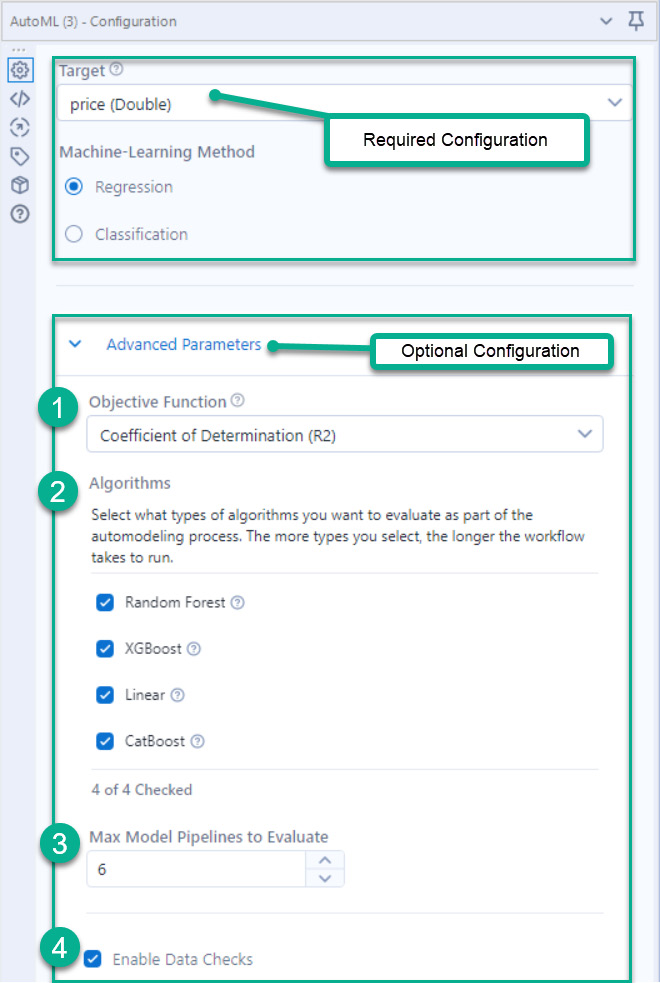
Figure 8.10 – Configuration of the AutoML tool

In Required Configuration, you select what your target field is. For our dataset and model, we are targeting the Price field. The tool will then default to the ML method of either Regression or Classification, based on the target field's data type. Of course, you can override this default option.

Optional Configuration is hidden in a collapsed menu. Once you have expanded the Advanced Parameters menu, there are four sections you can modify:

• Objective Function: You target this function to decide which model performs the best. Depending on whether you complete a regression or classification analysis, you will get a different outcome. Each of these metrics has its own benefits and drawbacks, but using the default value is good for beginning your ML model building.
• Algorithms to test: There are four models that Alteryx will test as part of the AutoML process. These models provide a common starting point for building your model, which you can choose to train or exclude. The algorithms you can apply are as follows:
  • Random Forest
  • XGBoost
  • Linear
  • CatBoost
• Max Model Pipelines to Evaluate: Part of the process will involve a series of data transformations, such as one-hot encoding. This option will allow you to tune how many different pipelines you want to test and then build your model.
• Enable Data Checks: Alteryx Designer can apply the default data checks from the EvalML Python package released by Alteryx. You can find the documentation for EvalML at https://evalml.alteryx.com/en/stable/user_guide/data_checks.html.

Once you run the AutoML tool, it will return a single record with the model that performs the best based on your objective function, along with the associated performance metrics. You will then connect the output to a Predict tool, along with the dataset you want to predict with the model.

The AutoML tool only provides the model for use in a subsequent step or another Alteryx workflow. It does not return any details about the creation of the model or tuning in the model for building further with that model as the starting point. Nevertheless, this model is great as a baseline for further testing.

Configuring an Assisted Modeling workflow

The Assisted Modeling tool is a more guided analysis than a black-box approach. With the Assisted Modeling tool, you will get feedback on the process and what is happening at each step in the model building process. Then, when the modeling is complete, the tool will output each pipeline model for use with a Predict tool (in a similar manner to the AutoML tool).

When using the Assisted Modeling tool, you are first prompted to choose between an Assisted or Expert process. The Expert process asks you to choose the Target field in your dataset to try and predict. With this option selected, you can use the other ML tools to create an ML workflow.

The second option to choose is the Assisted process. After selecting the Target variable, you can then choose the amount of interaction you will have in the pipeline creation. The Step-by-Step option allows you to review any transformations and recommendations in the Assisted Modeling tool, while the Automatic option will apply all recommendations and generate the leaderboard for you.

Before you exit the tool, you view the leaderboard, where you can see the performance comparisons between each tested model. The comparison metrics include Accuracy, Balanced Accuracy, and other accuracy metrics depending on whether the model is a classification or a regression model. Finally, you see the recommended model from this view and you can select one or more of the models as an Alteryx pipeline snippet.

The Assisted Modeling tool is an excellent method for continuing your ML project. It provides more feedback regarding the model you are building and more flexibility in creating future iterations of the ML model.

Building workflows with R-based predictive tools

In cases where the guided process of Intelligence Suite is not adequate, or you don't have access to Intelligence Suite, you can use R-based macros. R-based macros require a separate install, with the installer taken from the same download location as the Alteryx Designer install. This second install is required due to the license for the R language but has no additional cost associated with its use.

Installing R-Based Predictive Tools

If you need to install the R-tools for predictive analysis, you can access the installer directly from https://downloads.alteryx.com or by following the link in the navigation to the Options menu in the menu bar of Alteryx and clicking on Download Predictive Tools.

Once you have installed the R tools, you can start building a workflow using the R-based predictive tools. These tools will require a better understanding of the process you are applying.

The first step when using the R-based tools is to train the model. The training process requires configuring each model you want to create, such as a linear regression model or a boosted model. Each model has its own configuration parameters that you can tune and explain in a separate book. Therefore, when using the R-based tools, you must understand what model you are creating and what each parameter can do.

Each model tool has a consistent set of outputs:

• The Object output (O): This output is the R model the scoring tool uses to make predictions.
• The Report output (R): This output has a static report with the performance metrics and configuration of the model. This report is what you need to examine to understand the performance of each model.
• The Interactive output (I): Some of the R-based models also have an interactive output (I). This output contains an interactive version of the report generated by the model tool, making exploring the performance of that model configuration easier to undertake.

When building an ML pipeline, you need to make multiple models and evaluate which performs the best. You will have to decide what model to use with your expertise and manually compare each workflow's performance. You can make a comparison by using the Model Comparison tool, and this can be downloaded from the community (https://community.alteryx.com/t5/Public-Community-Gallery/Model-Comparison/ta-p/878736).

This tool will allow you to take the trained R models from multiple tools. The models need to be unioned into a single field for the model comparison to generate predictions for each option. The models can be from different algorithms, for example, comparing a random forest model with linear regression, or from the same algorithm with different configurations, such as changing the tree pruning depth in a random forest. As mentioned, these different configurations will be unique to each tool, but will give you the flexibility to customize the algorithm for your application.

Creating a custom Python or R script in a workflow

The final method for creating an ML pipeline is to use custom code tools. The ability to implement your scripts within Alteryx allows you to take the results of any methods we have already discussed and customize them even further for your application. Alternatively, you can create a unique model using different R and Python data science communities.

The R tool and the Python tool implement the scripting functionality in different processes based on when they were created.

Using the R tool

The R tool was the original predictive tool created by Alteryx and uses a more straightforward text editing scripting process, with the ability to add standardized Alteryx-specific snippets to the code. The following screenshot shows the Insert Code menu with the different options available:

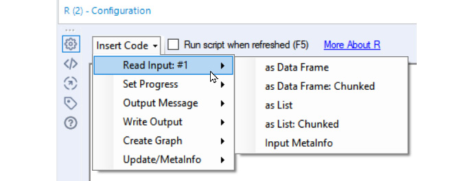
Figure 8.11 – R tool Insert Code menu

The R tool will take any R code available and process that with the data you feed into the tool. It allows you to leverage the analytical capabilities of Alteryx and then extend that capability with the expertise and packages in the R community. A limitation of the tool is that it does not do any code checking while you are writing the script; it is only evaluated at runtime. Additionally, you must run your entire workflow to run the code. If you have any slow upstream processes, they will run every time you test a code section. The simplest solution to this is to output an intermediate dataset as a .yxdb file and run the R code on only that dataset (without the processing with every test).

If you want to use any non-standard packages, the best method for installing them is to use the Install R Packages tool from the community (https://community.alteryx.com/t5/Public-Community-Gallery/Install-R-Packages/ta-p/878756). This tool will install the new packages into the R instance that Alteryx uses and place them in the library for you to use in the future. Alternatively, you could install the packages directly in the R console with the install.packages() function or any alternative method you might use in your R application.

If you want to use any custom package in a server application, you will need to run the same process on your server to make it available there.

Using the Python tool

The newer Python tool uses a Jupyter notebook instance for the Python editor. This method gives the advantage of having a cell-based code editor, thereby allowing the easier running of code snippets during your Python development.

The following screenshot shows the initial Python tool window before you add any code:

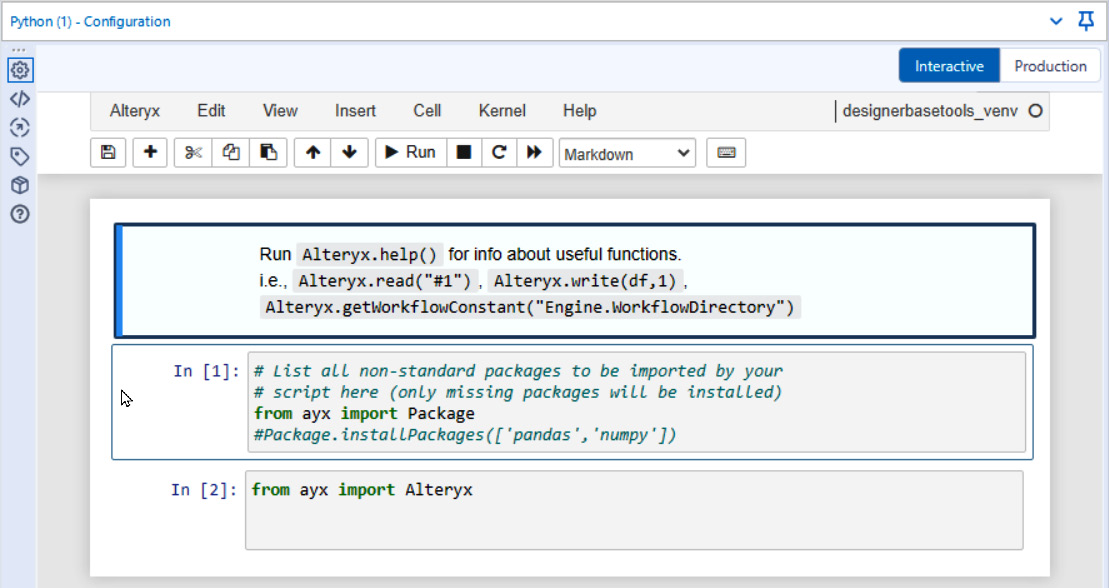
Figure 8.12 – Initial loading view of the Python tool

In this view, there are three initial cells created. The first is a markdown cell with information on how to access the Alteryx-specific Python functions, such as Alteryx.read("#1"), for importing the dataset from connection #1.

The next two cells are Python code cells, showing how to import and install packages for the Python tool. The Alteryx module from the ayx package is required to access the Alteryx data engine from the Python code in the Python tool. The Packages module lets you install a new package in the Alteryx workflow.

We now understand the three methods for creating an ML project in Alteryx. You can start with a hands-off process or a guided method using Intelligence Suite. You can then customize the pipeline more with the R-based Python tools. Finally, you can take complete control of the code with the R and Python tools. This progression shows how Alteryx can leverage the no-code, low-code, or code-friendly development options for creating your workflow.

With this understanding, we can learn the method for building standardized reports and reporting objects for delivering your insights.

Summary

In this chapter, we learned how to perform advanced analysis on our dataset. We took the skills learned in Chapter 7, Extracting Value, and extended our analysis to acquire a more in-depth understanding of the data. We started with spatial analysis and learned how to create spatial objects before finding the relationships between the geographic information that appear in your data.

Next, we learned the different methods for creating ML models with Alteryx. We found how to develop black-box and guided models for quickly beginning a data science project. We then saw the different methods for gaining control over the data science process using the R-based tools and taking complete control with the R or Python tools.

This chapter also concludes Part 2, Functional Steps in DataOps. First, we learned how to build a data pipeline and apply the DataOps method to create workflows. Then, we learned how to access raw datasets and process them into valuable final datasets. We have also learned how to manage the output of the created datasets. Finally, we extracted value from our data with spatial analytics, ML models, and building reports.

We will learn how to manage and govern your Alteryx data engineering environment in the next part. The next chapter will focus on applying tests to your workflows and enhancing this with continuous integration practices. We will also build a monitoring insight report to ensure that our data quality remains high.