11
Advanced Sequential Modeling Algorithms
An algorithm is a sequence of instructions that, if followed, will solve a problem.
—Unknown
In the last chapter we looked into the core principles of sequential models. It provided an introductory overview of their techniques and methodologies. The sequential modeling algorithms discussed in the last chapter had two basic restrictions. First, the output sequence was required to have the same number of elements as the input sequence. Second, those algorithms can process only one element of an input sequence at a time. If the input sequence is a sentence, it means that the sequential algorithms discussed so far can “attend,” or process, only one word at a time. To be able to better mimic the processing capabilities of the human brain, we need much more than that. We need complex sequential models that process an output with different lengths to the input, and which can attend to more than one word of a sentence at the same time, removing this information bottleneck.
In this chapter, we will delve deeper into the advanced aspects of sequential models to understand the creation of complex configurations. We’ll start by breaking down key elements, such as autoencoders and Sequence-to-Sequence (Seq2Seq) models. Next, we will look at attention mechanisms and transformers, which are pivotal in the development of Large Language Models (LLMs), which we will then study.
By the end of this chapter, you will have gained a comprehensive understanding of these advanced structures and their significance in the realm of machine learning. We will also provide insights into the practical applications of these models.
The following topics are covered in this chapter:
- Introduction to autoencoders
- Seq2Seq models
- Attention mechanisms
- Transformers
- LLMs
- Deep and wide architectures
First, let’s explore an overview of advanced sequential models.
The evolution of advanced sequential modeling techniques
In Chapter 10, Understanding Sequential Models, we touched upon the foundational aspects of sequential models. While they serve numerous use cases, they face challenges in grasping and producing the complex intricacies of human language.
We’ll begin our journey by discussing autoencoders. Introduced in the early 2010s, autoencoders provided a refreshing approach to data representation. They marked a significant evolution in natural language processing (NLP), transforming how we thought about data encoding and decoding. But the momentum in NLP didn’t stop there. By the mid-2010s, Seq2Seq models entered the scene, bringing forth innovative methodologies for tasks such as language translation. These models could adeptly transform one sequence form into another, heralding an era of advanced sequence processing.
However, with the rise in data complexity, the NLP community felt the need for more sophisticated tools. This led to the 2015 unveiling of the attention mechanism. This elegant solution provided models the ability to selectively concentrate on specific portions of input data, enabling them to manage longer sequences more efficiently. Essentially, it allowed models to weigh the importance of different data segments, amplifying the relevant and diminishing the less pertinent.
Building on this foundation, 2017 saw the advent of the transformer architecture. Fully leveraging the capabilities of attention mechanisms, transformers set new benchmarks in NLP.
These advancements culminated in the development of Large Language Models (LLMs). Trained on vast and diverse textual data, LLMs can both understand and generate nuanced human language expressions. Their unparalleled prowess is evident in their widespread applications, from healthcare diagnostics to algorithmic trading in finance.
In the sections that follow, we’ll unpack the intricacies of autoencoders—from their early beginnings to their central role in today’s advanced sequential models. Prepare to deep dive into the mechanisms, applications, and evolutions of these transformative tools.
Exploring autoencoders
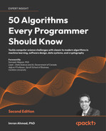
Autoencoders occupy a unique niche in the landscape of neural network architectures, playing a pivotal role in the narrative of advanced sequential models. Essentially, an autoencoder is designed to create a network where the output mirrors its input, implying a compression of the input data into a more succinct, lower-dimensional latent representation.
The autoencoder structure can be conceptualized as a dual-phase process: the encoding phase and the decoding phase.
Consider the following diagram:
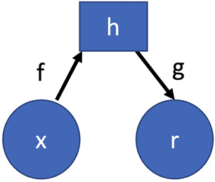
Figure 11.1: Autoencoder architecture
In this diagram we make the following assumptions:
- x corresponds to the input data
- h is the compressed form of our data
- r denotes the output, a recreation or approximation of x
We can see that the two phases are represented by f and g. Let’s look at them in more detail:
- Encoding (f): Described mathematically as h = f(x). In this stage, the input, represented as x, transforms into a condensed, hidden representation labeled h.
- Decoding (g): During this phase, represented as r = g(h), the compacted h is unraveled, aiming to reproduce the initial input.
When training an autoencoder, the goal is to perfect h, ensuring it encapsulates the essence of the input data. In achieving a high-quality h, we ensure the recreated output r mirrors the original x with minimal loss. The objective is not just to reproduce but also to train an h that’s streamlined and efficient in this reproduction task.
Coding an autoencoder
The Modified National Institute of Standards and Technology (MNIST) dataset is a renowned database of handwritten digits, consisting of 28x28 pixel grayscale images representing numbers from 0 to 9. It has been widely used as a benchmark for machine learning algorithms. More information and access to the dataset can be found at the official MNIST website. For those interested in accessing the dataset, it’s available at the official MNIST repository hosted by Yann LeCun: yann.lecun.com/exdb/mnist/. Please note that an account may be required to download the dataset.
In this section, we’ll employ an autoencoder to reproduce these handwritten digits. The unique feature of autoencoders is their training mechanism: the input and the target output are the same image. Let’s break this down.
First, there is the training phase, where the following steps occur:
- The MNIST images are provided to the autoencoder.
- The encoder segment compresses these images into a condensed latent representation.
- The decoder segment then tries to restore the original image from this representation. By iterating over this process, the autoencoder acquires the nuances of compressing and reconstructing, capturing the core patterns of the handwritten digits.
Second, there is the reconstruction phase:
- With the model trained, when we feed it new images of handwritten digits, the autoencoder will first encode them into its internal representation.
- Then, decoding this representation will yield a reconstructed image, which, if the training was successful, should closely match the original.
With the autoencoder effectively trained on the MNIST dataset, it becomes a powerful tool to process and reconstruct handwritten digit images.
Setting up the environment
Before diving into the code, essential libraries must be imported. TensorFlow will be our primary tool, but for data handling, libraries like NumPy may be pivotal:
import tensorflow as tf
Data preparation
Next, we’ll segregate the dataset into training and test segments and then normalize them:
# Load dataset
(x_train, _), (x_test, _) = tf.keras.datasets.mnist.load_data()
# Normalize data to range [0, 1]
x_train, x_test = x_train / 255.0, x_test / 255.0
Note that the division by 255.0 is to normalize our grayscale image data, a step that optimizes the learning process.
Model architecture
Designing the autoencoder involves making decisions about the layers, their sizes, and activation functions. Here, the model is defined using TensorFlow’s Sequential and Dense classes:
model = tf.keras.Sequential([
    tf.keras.layers.Flatten(input_shape=(28, 28)),
    tf.keras.layers.Dense(32, activation='relu'),
    tf.keras.layers.Dense(784, activation='sigmoid'),
    tf.keras.layers.Reshape((28, 28))
])
Flattening the 28x28 images gives us a 1D array of 784 elements, hence the input shape.
Compilation
After the model is defined, it’s compiled with a specified loss function and optimizer. Binary cross-entropy is chosen due to the binary nature of our grayscale images:
model.compile(loss='binary_crossentropy', optimizer='adam')
Training
The training phase is initiated with the fit method. Here, the model learns the nuances of the MNIST handwritten digits:
model.fit(x_train, x_train, epochs=10, batch_size=128,
          validation_data=(x_test, x_test))
Prediction
With a trained model, predictions (both encoding and decoding) can be executed as follows:
encoded_data = model.predict(x_test)
decoded_data = model.predict(encoded_data)
Visualization
Let us now visually compare the original images with their reconstructed counterparts. The following script showcases a visualization procedure that displays two rows of images:
n = 10  # number of images to display
plt.figure(figsize=(20, 4))
for i in range(n):
    # Original images
    ax = plt.subplot(2, n, i + 1)
    plt.imshow(x_test[i].reshape(28, 28) , cmap='gray')
    ax.get_xaxis().set_visible(False)
    ax.get_yaxis().set_visible(False)
    # Reconstructed images
    ax = plt.subplot(2, n, i + 1 + n)
    plt.imshow(decoded_data[i].reshape(28, 28) , cmap='gray')
    ax.get_xaxis().set_visible(False)
    ax.get_yaxis().set_visible(False)
plt.show()
The following screenshot shows the outputted reconstructed images:

Figure 11.2: The original test images (top row) and the post-reconstruction by the autoencoder (bottom row)
The top row presents the original test images, while the bottom row exhibits the post-reconstruction images made by the autoencoder. Through this side-by-side comparison, we can discern the efficacy of our model in preserving the intrinsic features of the input.
Let us now discuss Seq2Seq models.
Understanding the Seq2Seq model
Following our exploration of autoencoders, another groundbreaking architecture in the realm of advanced sequential models is the Seq2Seq model. Central to many state-of-the-art natural language processing tasks, the Seq2Seq model exhibits a unique capability: transforming an input sequence into an output sequence that may differ in length. This flexibility allows it to excel in challenges like machine translation, where the source and target sentences can naturally differ in size.
Refer to Figure 11.3, which visualizes the core components of a Seq2Seq model:
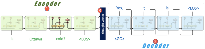
Figure 11.3: Illustration of the Seq2Seq model architecture
Broadly, there are three main elements:
- Encoder: Processes the input sequence
- Thought vector: A bridge between the encoder and decoder
- Decoder: Generates the output sequence
Let us explore them one by one.
Encoder
The encoder is shown as ![]() in Figure 11.3. As we can observe, it is an input Recurrent Neural Network (RNN) that processes the input sequence. The input sentence in this case is a three-word sentence: Is Ottawa cold? It can be represented as:
in Figure 11.3. As we can observe, it is an input Recurrent Neural Network (RNN) that processes the input sequence. The input sentence in this case is a three-word sentence: Is Ottawa cold? It can be represented as:
X = {x<1>, x<2>,… …., x<L1>}
The encoder traverses through this sequence until it encounters an End-Of-Sentence (<EOS>) token, indicating the conclusion of the input. It will be positioned at timestep L1.
Thought vector
Throughout the encoding phase, the RNN updates its hidden state, denoted by h<t>. The final hidden state, captured at the end of the sequence h<L1>, is relayed to the decoder. This final state is termed the thought vector, coined by Geoffrey Hinton in 2015. This compact representation captures the essence of the input sequence. The thought vector is shown as ![]() in Figure 11.3.
in Figure 11.3.
Decoder or writer
Upon completion of the encoding process, a <GO> token signals the decoder to commence. Using the encoder’s final hidden state h<L1> as its initial input, the decoder, an output RNN, begins constructing the output sequence, Y = {y<1>, y<2>,… …., y<L2>}. In the context of Figure 11.3, this output sequence translates to the sentence: Yes, it is.
Special tokens in Seq2Seq
While <EOS> and <GO> are essential tokens within the Seq2Seq paradigm, there are others worth noting:
<UNK>: Standing for unknown, this token replaces infrequent words, ensuring the vocabulary remains manageable.<PAD>: Used for padding shorter sequences, this token standardizes sequence lengths during training, enhancing the model’s efficacy.
A salient feature of the Seq2Seq model is its ability to handle variable sequence lengths, meaning input and output sequences can inherently differ in size. This flexibility, combined with its sequential nature, makes Seq2Seq a pivotal architecture in the advanced modeling landscape, bridging our journey from autoencoders to more complex, nuanced sequential processing systems.
Having traversed the foundational realms of autoencoders and delved deep into the Seq2Seq models, we now need to understand the limitations of the encoder-decoder framework.
The information bottleneck dilemma
As we have learned, the heart of traditional Seq2Seq models is the thought vector, h<L1> . This is the last hidden state from the encoder, which serves as the bridge to the decoder. This vector is tasked with encapsulating the entirety of the input sequence, X. The simplicity of this mechanism is both its strength and its weakness. This weakness is highlighted when sequences grow longer; compressing vast amounts of information into a fixed-size representation becomes increasingly formidable. This is termed the information bottleneck. No matter the richness or complexity of the input, the fixed-length memory constraint means only so much can be relayed from the encoder to the decoder.
To learn how this problem has been addressed, we need to shift our focus from Seq2Seq models to the attention mechanism.
Understanding the attention mechanism
Following the challenges presented by the fixed-length memory in traditional Seq2Seq models, 2014 marked a revolutionary step forward. Dzmitry Bahdanau, KyungHyun Cho, and Yoshua Bengio proposed a transformative solution: the attention mechanism. Unlike earlier models that tried (often in vain) to condense entire sequences into limited memory spaces, attention mechanisms enabled models to hone in on specific, relevant parts of the input sequence. Picture it as a magnifying glass over only the most critical data at each decoding step.
What is attention in neural networks?
Attention, as the adage goes, is where focus goes. In the realm of NLP and particularly in the training of LLMs, attention has garnered significant emphasis. Traditionally, neural networks processed input data in a fixed sequence, potentially missing out on the relevance of context. Enter attention—a mechanism that weighs the importance of different input data, focusing more on what’s relevant.
Basic idea
Just as humans pay more attention to salient parts of an image or text, attention mechanisms allow neural models to focus on more relevant parts of the input data. It effectively tells the model where to “look” next.
Example
Inspired by my recent journey to Egypt, which felt like a voyage back in time, consider the expressive and symbolic language of ancient Egypt: hieroglyphs.
Hieroglyphs were much more than mere symbols; they were an intricate fusion of art and language, representing multifaceted meanings. This system, with its vast array of symbols, exemplifies the foundational principles of attention mechanisms in neural networks.

Figure 11.4: Giza’s prominent pyramids - Khufu and Khafre, accompanied by inscriptions in the age-old Egyptian script, “hieroglyphs” (photographs taken by the author)
For instance, an Egyptian scribe wishes to convey news about an anticipated grand festival by the Nile. Out of the thousands of hieroglyphs available:
 The Ankh hieroglyph, symbolizing life, captures the festival’s vibrancy and celebratory spirit.
 The Was symbol, resembling a staff, hints at authority or the Pharaoh’s pivotal role in the celebrations.
 An illustration of the Nile, central to Egyptian culture, pinpoints the festival’s venue.
However, to communicate the festival’s grandeur and importance, not all symbols would hold equal weight. The scribe would have to emphasize or repeat specific hieroglyphs to draw attention to the most crucial aspects of the message.
This selective emphasis is parallel to neural network attention mechanisms.
Three key aspects of attention mechanisms
In neural networks, especially within NLP tasks, attention mechanisms play a crucial role in filtering and focusing on relevant information. Here, we’ll distill the primary facets of attention into three main components: contextual relevance, symbol efficiency, and prioritized focus:
- Contextual relevance:
- Overview: At its core, attention aims to allocate more importance to certain parts of the input data that are deemed more relevant to the task at hand.
- Deep dive: Take a simple input like “The grand Nile festival.” In this context, attention mechanisms might assign higher weights to the words “Nile” and “grand.” This isn’t because of their general significance but due to their task-specific importance. Instead of treating every word or input with uniform importance, attention differentiates and adjusts the model’s focus based on context.
- In practice: Think of this as a spotlight. Just as a spotlight on a stage illuminates specific actors during crucial moments while dimming others, attention shines a light on specific input data that holds more contextual value.
- Symbol efficiency:
- Overview: The ability of attention to condense vast amounts of information into digestible, critical segments.
- Deep dive: Hieroglyphs can encapsulate complex narratives or ideas within singular symbols. Analogously, attention mechanisms, by assigning varied weights, can determine which segments of the data contain maximal information and should be processed preferentially.
- In practice: Consider compressing a large document into a succinct summary. The summary retains only the most critical information, mirroring the function of attention mechanisms that extract and prioritize the most pertinent data from a larger input.
- Prioritized focus:
- Overview: Attention mechanisms don’t distribute their focus uniformly. They are designed to prioritize segments of input data based on their perceived relevance to the task.
- Deep dive: Drawing inspiration from our hieroglyph example, just as an Egyptian scribe might emphasize the “Ankh” symbol when wanting to convey the idea of life or celebration, attention mechanisms will adjust their focus (or weights) to specific parts of the input that are more relevant.
- In practice: It’s akin to reading a research paper. While the entire document holds value, one might focus more on the abstract, conclusion, or specific data points that align with their current research needs.
Thus, the attention mechanism in neural networks emulates the selective focus humans naturally employ when processing information. By understanding the nuances of how attention prioritizes and processes data, we can better design and interpret neural models.
A deeper dive into attention mechanisms
Attention mechanisms can be thought of as an evolved form of communication, much like hieroglyphs were in ancient times. Traditionally, an encoder sought to distill an entire input sequence into one encapsulating hidden state. This is analogous to an Egyptian scribe trying to convey an entire event using a single hieroglyph. While possible, it’s challenging and may not capture the event’s full essence.
Now, with the enhanced encoder-decoder approach, we have the luxury of generating a hidden state for every step, offering a richer tapestry of data for the decoder. But referencing every single hieroglyph (or state) at once would be chaotic, like a scribe using every symbol available to describe a single event by the Nile. That’s where attention comes in.
Attention allows the decoder to prioritize. Just as a scribe might focus on the “Ankh” hieroglyph to signify life and vitality, or the “Was” staff to represent power, or even depict the Nile itself to pinpoint a location, the decoder assigns varying weightage to each encoder state. It decides which parts of the input sequence (or which hieroglyphs) deserve more emphasis. Using our translation example, when converting “Transformers are great!” to “Transformatoren sind grossartig!”, the mechanism emphasizes aligning “great” with “grossartig,” ensuring the core sentiment remains intact.
This selective focus, whether in neural network attention mechanisms or hieroglyphic storytelling, ensures precision and clarity in the conveyed message.
Figure 11.5: RNNs employing an encoder-decoder structure enhanced with an attention mechanism
The challenges of attention mechanisms
While incorporating attention with RNNs offers notable improvements, it’s not a silver bullet. One significant hurdle is computational cost. The act of transferring multiple hidden states from encoder to decoder demands substantial processing power.
However, as with all technological progress, solutions continually emerge. One such advancement is the introduction of self-attention, a cornerstone of transformer architectures. This innovative variant refines the attention process, making it more efficient and scalable.
Delving into self-attention
Let’s consider again the ancient art of hieroglyphs, where symbols were chosen intentionally to convey complex messages. Self-attention operates in a similar manner, determining which parts of a sequence are vital and should be emphasized.
Illustrated in Figure 11.6 is the beauty of integrating self-attention within sequential models. Think of the bottom layer, churning with bidirectional RNNs, as the foundational stones of a pyramid. They generate what we call the context vector (c2), a summary, much like a hieroglyph would for an event.
Each step or word in a sequence has its weightage, symbolized as α. These weights interact with the context vector, emphasizing the importance of certain elements over others.
Imagine a scenario wherein the input Xk represents a distinct sentence, denoted as k, which spans a length of L1. This can be mathematically articulated as:
![]()
Here, every element, ![]() , represents a word or token from sentence k: the superscript <t> indicates its specific position or timestep within that sentence.
, represents a word or token from sentence k: the superscript <t> indicates its specific position or timestep within that sentence.
Attention weights
In the realm of self-attention, attention weights play a pivotal role, acting like a compass pointing to which words are essential. They assign an “importance score” to each word when generating the context vector.
To bring this into perspective, consider our earlier translation example: “Transformers are great!” translated to “Transformatoren sind grossartig!”. When focusing on the word “Transformers”, the attention weights might break down like this:
- α2,1: Measures the relationship between “Transformers” and the beginning of the sentence. A high value here indicates that the word “Transformers” significantly relies on the beginning for its context.
- α2,2: Reflects how much “Transformers” emphasizes its inherent meaning.
- α2,3 and α2,4: These weigh how much “Transformers” takes into context the words “are” and “great!”, respectively. High scores here mean that “Transformers” is deeply influenced by these surrounding words.
During training, these attention weights are constantly adjusted and fine-tuned. This ongoing refinement ensures our model understands the intricate dance between words in a sentence, capturing both the explicit and subtle connections.

Figure 11.6: Integrating self-attention in sequential models
Before we delve deeper into the mechanisms of self-attention, it’s vital to understand the key pieces that come together in Figure 11.6.
Encoder: bidirectional RNNs
In the last chapter we investigated the main architectural building blocks of unidirectional RNN and its variants. Bidirectional RNNs were invented to address that need (Schuster and Paliwal, 1997). We also identified a deficiency in unidirectional RNNs, as they are only capable of carrying the context in one direction.
For an input sequence, say X, the bidirectional RNN first reads it from the start to the end, and then from the end back to the start. This dual approach helps capture information based on preceding and succeeding elements. For each timestep, we get two hidden states: ![]() for the forward direction and
for the forward direction and ![]() for the backward one. These states are merged into a single one for that timestep, represented by:
for the backward one. These states are merged into a single one for that timestep, represented by:
![]()
For instance, if ![]() and
and ![]() are 64-dimensional vectors, the resulting h<t2> is 128-dimensional. This combined state is a detailed representation of the sequence context from both directions.
are 64-dimensional vectors, the resulting h<t2> is 128-dimensional. This combined state is a detailed representation of the sequence context from both directions.
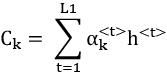
Thought vector
The thought vector, here symbolized as Ck, is a representation of the input Xk. As we have learned, its creation is an attempt to capture the sequencing patterns, context, and state of each element in Xk.
In our preceding diagram it is defined as:
![]()
Where ![]() are attention weights for timestep t that are refined during training.
are attention weights for timestep t that are refined during training.
Using the summation notation, it can be expressed as:
Decoder: regular RNNs
Figure 11.5 shows the decoder connected through the thought vector to the encoder.
The output of the decoder for a certain sentence k is represented by:
![]()
Note that the output has a length of L2, which is different from the length of the input sequence, which was L1.
Training versus inference
In the training data for a certain input sequence k, we have the expected output vector representing the ground truth, which is represented by a vector Yk. This is:
![]()
At each timestep, the decoder’s RNN gets three inputs:
 : The previous hidden state
- Ck: The thought vector for sequence k
 : The previous word in the ground truth vector Yk
However, during inference, as there’s no prior ground truth available, the decoder’s RNN uses the prior output word, ![]() , instead.
, instead.
Now that we have learned how self-attention addresses the challenges faced by attention mechanisms and the basic operations it involves, we can move our attention to the next major advancement in sequential modeling: transformers.
Transformers: the evolution in neural networks after self-attention
Our exploration into self-attention revealed its powerful capability to reinterpret sequence data, providing each word with a contextual understanding based on its relationships with other words. This principle set the stage for an evolutionary leap in neural network designs: the transformer architecture.
Introduced by the Google Brain team in their 2017 paper, Attention is All You Need (https://arxiv.org/abs/1706.03762), the transformer architecture is built upon the very essence of self-attention. Before its advent, RNNs were the go-to. Picture RNNs as diligent librarians reading an English sentence to translate it into German, word by word, ensuring the context is relayed from one word to the next. They’re reliable for short texts but can stumble when sentences get too long, misplacing the essence of earlier words.

Figure 11.7: Encoder-decoder architecture of the original transformer
Transformers are a fresh approach to sequence data. Instead of a linear, word-by-word progression, transformers, armed with advanced attention mechanisms, comprehend an entire sequence in a single glance. It’s like instantly grasping the sentiment of a whole paragraph rather than piecing it together word by word. This holistic view ensures a richer, all-encompassing understanding, celebrating the nuanced interplay between words.
Self-attention is central to the transformer’s efficiency. While we touched upon this in the previous section, it’s worth noting how pivotal it is here. Each layer of the network, through self-attention, can resonate with every other part of the input data. As depicted in Figure 11.7, the transformer architecture employs self-attention for both its encoder and decoder segments, which then feed into neural networks (also known as feedforward neural networks (FFNNs)). Beyond being more trainable, this setup has catalyzed many of the recent breakthroughs in NLP.
To illustrate, consider Ancient Egypt: An Enthralling Overview of Egyptian History, by Billy Wellman. Within it, the relationships between early pharaohs like Ramses and Cleopatra and pyramid construction are vast and intricate. Traditional models might stumble with such expansive content.
Why transformers shine
The transformer architecture, with its self-attention mechanism, emerges as a promising solution. When encountering a term like “pyramids,” the model can, using self-attention, assess its relevance to terms like “Ramses” or “Cleopatra,” irrespective of their position. This ability to attend to various input parts demonstrates why transformers are pivotal in modern NLP.
A Python code breakdown
Here’s a simplified version of how the self-attention mechanism can be implemented:
import numpy as np
def self_attention(Q, K, V):
    """
    Q: Query matrix
    K: Key matrix
    V: Value matrix
    """

    # Calculate the attention weights
    attention_weights = np.matmul(Q, K.T)

    # Apply the softmax to get probabilities
    attention_probs = np.exp(attention_weights) / np.sum(np.exp(attention_weights), axis=1, keepdims=True)

    # Multiply the probabilities with the value matrix to get the output
    output = np.matmul(attention_probs, V)

    return output
# Example
Q = np.array([[1, 0, 1], [0, 2, 0], [1, 1, 0]])  # Example Query
K = np.array([[1, 0, 1], [0, 2, 0], [1, 1, 0]])  # Key matrix
V = np.array([[0, 2, 0], [1, 0, 1], [0, 1, 2]])  # Value matrix
output = self_attention(Q, K, V)
print(output)
Output:
[[0.09003057 1.57521038 0.57948752]
 [0.86681333 0.14906291 1.10143419]
 [0.4223188  0.73304361 1.26695639]]
This code is a basic representation, and the real transformer model uses a more optimized and detailed approach, especially when scaling for larger sequences. But the essence is the dynamic weighting of different words in the sequence, allowing the model to bring in contextual understanding.
Understanding the output
- The first row,
[0.09003057 1.57521038 0.57948752], corresponds to the weighted combination of the V matrix for the first word in the query (in this case, represented by the first row of the Q matrix). This means when our model encounters the word represented by this query, it will focus 9% on the first word, 57.5% on the second word, and 57.9% on the third word from the V matrix to derive contextual understanding. - The second row,
[0.86681333 0.14906291 1.10143419], is the attention result for the second word in the query. It focuses 86.6% on the first word, 14.9% on the second, and 110.1% on the third from the V matrix. - The third row,
[0.4223188 0.73304361 1.26695639], is for the third word in the query. It has attention weights of 42.2%, 73.3%, and 126.7%, respectively, for the words in the V matrix.
Having reviewed transformers, their place in sequential modeling, their code, and their output, we can consider the next major development in NLP. Next, let us look at LLMs.
LLMs
LLMs are the next evolutionary step after transformers in the world of NLP. They’re not just beefed-up older models; they represent a quantum leap. These models can handle vast amounts of text data and perform tasks previously thought to be reserved for human minds.
Simply put, LLMs can produce text, answer questions, and even code. Picture chatting with software and it replying just like a human, catching subtle hints and recalling earlier parts of the conversation. That’s what LLMs offer.
Language models (LMs) have always been the backbone of NLP, helping in tasks ranging from machine translation to more modern tasks like text classification. While the early LMs relied on RNNs and Long Short-Term Memory (LSTM) structures, today’s NLP achievements are primarily due to deep learning techniques, especially transformers.
The hallmark of LLMs? Their capacity to read and learn from vast quantities of text. Training one from scratch is a serious undertaking, requiring powerful computers and lots of time. Depending on factors like the model’s size and the amount of training data—say, from giant sources like Wikipedia or the Common Crawl dataset—it could take weeks or even months to train an LLM.
Dealing with long sequences is a known challenge for LLMs. Earlier models, built on RNNs and LSTMs, faced issues with lengthy sequences, often losing vital details, which hampered their performance. This is where we start to see the role of attention come into play. Attention mechanisms act as a torch, illuminating essential sections of long inputs. For example, in a text about car advancements, attention makes sure the model recognizes and focuses on the major breakthroughs, no matter where they appear in the text.
Understanding attention in LLMs
Attention mechanisms have become foundational in the neural network domain, particularly evident in LLMs. Training these mammoth models, laden with millions or even billions of parameters, is not a walk in the park. At their core, attention mechanisms are like highlighters, emphasizing key details. For instance, when processing a lengthy text on NLP’s evolution, LLMs can understand the overall theme, but attention ensures they don’t miss the critical milestones. Transformers utilize this attention feature, aiding LLMs in handling vast text stretches and ensuring contextual consistency.
For LLMs, context is everything. For example, if an LLM crafts a story starting with a cat, attention ensures that as the tale unfolds, the context remains. So instead of introducing unrelated sounds like “barking,” the story would naturally lean toward “purring” or “meowing.”
Training an LLM resembles running a supercomputer continuously for months, purely to process vast text quantities. And when the initial training is done, it’s only the beginning. Think of it like owning a high-end vehicle—you’d need periodic maintenance. Similarly, LLMs need frequent updates and refinements based on new data.
Even after training an LLM, the work isn’t over. For these models to remain effective, they need to keep learning. Imagine teaching someone English grammar rules and then throwing in slang or idioms—they need to adapt to these irregularities for a complete understanding.
Highlighting a historical shift, between 2017 and 2018, there was a notable change in the LLM landscape. Firms, including OpenAI, began leveraging unsupervised pretraining, paving the way for more streamlined models for tasks, like sentiment analysis.
Exploring the powerhouses of NLP: GPT and BERT
Universal Language Model Fine-Tuning (ULMFiT) set the stage for a new era in NLP. This method pioneered the reuse of pre-trained LSTM models, adapting them to a variety of NLP tasks, which saved both computational resources and time. Let’s break down its process:
- Pretraining: This is akin to teaching a child the basics of a language. Using extensive datasets like Wikipedia, the model learns the foundational structures and grammar of the language. Imagine this as equipping a student with general knowledge textbooks.
- Domain adaptation: The model then delves into specialized areas or genres. If the first step was about learning grammar, this step is like introducing the model to different genres of literature - from thrillers to scientific journals. It still predicts words, but now within specific contexts.
- Fine-tuning: Finally, the model is honed for specific tasks, such as detecting emotions or sentiments in a given text. This is comparable to training a student to write essays or analyze texts in depth.
2018’s LLM pioneers: GPT and BERT
2018 saw the rise of two standout models: GPT and BERT. Let us look into them in more detail.
Generative Pre-trained Transformer (GPT)
Inspired by ULMFiT, GPT is a model that leans on the decoder side of the transformer architecture. Visualize the vastness of human literature. If traditional models are trained with a fixed set of books, GPT is like giving a scholar access to an entire library, including the BookCorpus - a rich dataset with diverse, unpublished books. This allows GPT to draw insights from genres ranging from fiction to history.
Here’s an analogy: traditional models might know the plots of Shakespeare’s plays. GPT, with its extensive learning, would understand not only the plots but also the cultural context, character nuances, and the evolution of Shakespeare’s writing style over time.
Its focus on the decoder makes GPT a master of generating text that’s both relevant and coherent, like a seasoned author drafting a novel.
BERT (Bidirectional Encoder Representations from Transformers)
BERT revamped traditional language modeling with its “masked language modeling” technique. Unlike models that just predict the next word in a sentence, BERT fills in intentionally blanked-out or “masked” words, enhancing its contextual understanding.
Let’s put this into perspective. In a sentence like “She went to Paris to visit the ___,” conventional models might predict words that fit after “the,” such as “museum.” BERT, given “She went to Paris to visit the masked,” would aim to deduce that “masked” could be replaced by “Eiffel Tower,” understanding the broader context of a trip to Paris.
BERT’s approach offers a more rounded view of language, capturing the essence of words based on what precedes and follows them, elevating its language comprehension prowess.
The key to success when training an LLM lies in combining ‘deep’ and ‘wide’ learning architectures. Think of the ‘deep’ part as a specialist deeply focused on a subject, while the ‘wide’ approach is like a jack of all trades, understanding a bit of everything.
Using deep and wide models to create powerful LLMs
LLMs are intricately designed to excel at a rather specific task: predicting the next word in a sequence. It might seem simple at first, but to achieve this with high accuracy, models often draw inspiration from certain aspects of human learning.
The human brain, a marvel of nature, processes information by recognizing and abstracting common patterns from the surrounding environment. On top of this foundational understanding, humans then enhance their knowledge by memorizing specific instances or exceptions that don’t fit the usual patterns. Think of it as understanding a rule and then learning the outliers to that rule.
To infuse machines with this dual-layered learning approach, we need thoughtful machine learning architectures. A rudimentary method might involve training models solely on generalized patterns, sidelining the exceptions. However, to truly excel, especially in tasks like predicting the next word, models must be adept at grasping both the common patterns and the unique exceptions that punctuate a language.
While LLMs are not designed to fully emulate human intelligence (which is multifaceted and not solely about predicting sequences), they do borrow from human learning strategies to become proficient at their specific tasks.
LLMs are designed to understand and generate language by detecting patterns in vast amounts of text data. Consider the following basic linguistic guidelines:
- Ancient Egyptian hieroglyphs provide a fascinating example. In this early writing system, a symbol might represent a word, sound, or even a concept. For instance, while a single hieroglyph could denote the word “river,” a combination of hieroglyphs could convey a deeper meaning like “the life-giving Nile River.”
- Now, consider how questions are formed. Typically, they begin with auxiliary verbs. However, indirect inquiries, such as “I wonder if the Nile will flood this year” diverge from this conventional pattern.
To effectively predict the next word or phrase in a sequence, LLMs must master both the prevailing language norms and their occasional outliers.
Bottom of Form
Thus, combining deep and wide models (Figure 11.8) has been shown to improve the performance of models on a wide range of tasks. Deep models are characterized by having many hidden layers and are adept at learning complex relationships between input and output.
In contrast, wide models are designed to learn simple patterns in the data. By combining the two, it is possible to capture both the complex relationships and the simple patterns, leading to more robust and flexible models.
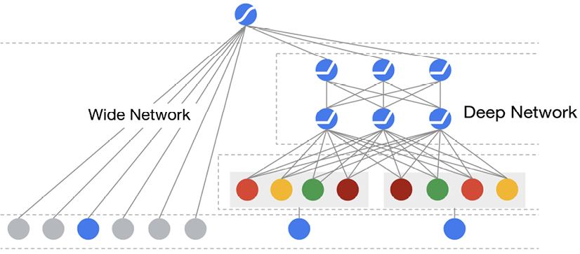
Figure 11.8: Architecture of deep and wide models
Incorporating exceptions into the training process is crucial for better generalization of models to new and unseen data. For example, a language model that is trained only on data that includes one meaning of a word may struggle to recognize other meanings when it encounters them in new data. By incorporating exceptions, the model can learn to recognize multiple meanings of a word, which can improve its performance on a variety of NLP tasks.
Deep architectures are typically used for tasks that require learning complex, hierarchical abstract representations of data. The features that exhibit generalizable patterns are called dense features. When we use deep architectures to formulate the rules, we call it learning by generalization. To build a wide and deep network, we connect the sparse features directly to the output node.
In the field of machine learning, combining deep and wide models has been identified as an important approach to building more flexible and robust models that can capture both complex relationships and simple patterns in data. Deep models excel at learning complex, hierarchical abstract representations of data, by having many hidden layers, where each layer processes the data and learns different features at different levels of abstraction. In contrast, wide models have a minimum number of hidden layers and are typically used for tasks that require learning simple, non-linear relationships in the data without creating any layer of abstraction.
Such patterns are represented through sparse features. When the wide part of the model has one or zero hidden layers, it can be used to memorize the examples and formulate exceptions. Thus, when wide architectures are used to formulate rules, we call it learning by memorization.
The deep and wide models can use the deep neural network to generalize patterns. Typically, this portion of the model will take lots of time to train. The wide partition and efforts to capture all the exceptions to these generalizations in real time are a part of the constant algorithmic learning process.
Summary
In this chapter we discussed advanced sequential models, which are advanced techniques designed to process input sequences, especially when the length of output sequences may differ from that of the input. Autoencoders, a type of neural network architecture, are particularly adept at compressing data. They work by encoding input data into a smaller representation and then decoding it back to resemble the original input. This process can be useful in tasks like image denoising, where noise from an image is filtered out to produce a clearer version.
Another influential model is the Seq2Seq model. It’s designed to handle tasks where input and output sequences have varying lengths, making it ideal for applications like machine translation. However, traditional Seq2Seq models face the information bottleneck challenge, wherein the entire context of an input sequence needs to be captured in a single, fixed-size representation. Addressing this, the attention mechanism was introduced, allowing models to focus on different parts of the input sequence dynamically. The transformer architecture, introduced in the paper Attention is All You Need, utilizes this mechanism, revolutionizing the processing of sequence data. Transformers, unlike their predecessors, can attend to all positions in a sequence simultaneously, capturing intricate relationships within the data. This innovation paved the way for LLMs, which have gained prominence for their human-like text-generation capabilities.
In the next chapter we will look into how to use recommendation engines.
Learn more on Discord
To join the Discord community for this book – where you can share feedback, ask questions to the author, and learn about new releases – follow the QR code below: