
3
Sorting and Searching Algorithms
In this chapter, we will look at the algorithms that are used for sorting and searching. This is an important class of algorithms that can be used on their own or can become the foundation for more complex algorithms. These include Natural Language Processing (NLP) and pattern-extracting algorithms. This chapter starts by presenting different types of sorting algorithms. It compares the performance of various approaches to designing a sorting algorithm. Then, some searching algorithms are presented in detail. Finally, a practical example of the sorting and searching algorithms presented in this chapter is studied.
By the end of this chapter, we should be able to understand the various algorithms that are used for sorting and searching, and we will be able to comprehend their strengths and weaknesses. As searching and sorting algorithms are the building blocks for many complex algorithms, understanding them in detail will help us better understand modern complex algorithms as well, as presented in the later chapters.
The following are the main concepts discussed in this chapter:
- Introducing sorting algorithms
- Introducing searching algorithms
- Performance analysis of sorting and searching algorithms
- Practical applications of sorting and searching
Let’s first look at some sorting algorithms.
Introducing sorting algorithms
The ability to efficiently sort and search items in a complex data structure is important as it is needed by many modern algorithms. The right strategy to sort and search data will depend on the size and type of the data, as discussed in this chapter. While the end result is exactly the same, the right sorting and searching algorithm will be needed for an efficient solution to a real-world problem. Thus, carefully analyzing the performance of these algorithms is important.
Sorting algorithms are used extensively in distributed data storage systems such as modern NoSQL databases that enable cluster and cloud computing architectures. In such data storage systems, data elements need to be regularly sorted and stored so that they can be retrieved efficiently.
The following sorting algorithms are presented in this chapter:
- Bubble sort
- Merge sort
- Insertion sort
- Shell sort
- Selection sort
But before we look into these algorithms, let us first discuss the variable-swapping technique in Python that we will be using in the code presented in this chapter.
Swapping variables in Python
When implementing sorting and searching algorithms, we need to swap the values of two variables. In Python, there is a standard way to swap two variables, which is as follows:
var_1 = 1
var_2 = 2
var_1, var_2 = var_2, var_1
print(var_1,var_2)
2, 1
This simple way of swapping values is used throughout the sorting and searching algorithms in this chapter.
Let’s start by looking at the bubble sort algorithm in the next section.
Bubble sort
Bubble sort is one of the simplest and slowest algorithms used for sorting. It is designed in such a way that the highest value in a list of data bubbles makes its way to the top as the algorithm loops through iterations. Bubble sort requires little runtime memory to run because all the ordering occurs within the original data structure. No new data structures are needed as temporary buffers. But its worst-case performance is O(N2), which is quadratic time complexity (where N is the number of elements being sorted). As discussed in the following section, it is recommended to be used only for smaller datasets. Actual recommended limits for the size of the data for the use of bubble sort for sorting will depend on the memory and the processing resources available but keeping the number of elements (N) below 1000 can be considered as a general recommendation.
Understanding the logic behind bubble sort
Bubble sort is based on various iterations, called passes. For a list of size N, bubble sort will have N-1 passes. To understand its working, let’s focus on the first iteration: pass one.
The goal of pass one is to push the highest value to the highest index (top of the list). In other words, we will see the highest value of the list bubbling its way to the top as pass one progresses.
Bubble sort’s logic is based on comparing adjacent neighbor values. If the value at a higher index is higher in value than the value at a lower index, we exchange the values. This iteration continues until we reach the end of the list. This is shown in Figure 3.1:
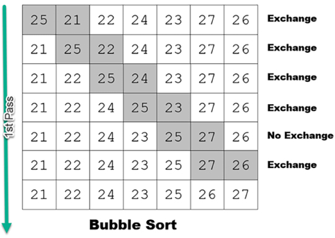
Figure 3.1: Bubble sort algorithm
Let’s now see how bubble sort can be implemented using Python. If we implement pass one of bubble sort in Python, it will look as follows:
list = [25,21,22,24,23,27,26]
last_element_index = len(list)-1
print(0,list)
for idx in range(last_element_index):
                if list[idx]>list[idx+1]:
                    list[idx],list[idx+1]=list[idx+1],list[idx]
                print(idx+1,list)
0 [25, 21, 22, 24, 23, 27, 26]
1 [21, 25, 22, 24, 23, 27, 26]
2 [21, 22, 25, 24, 23, 27, 26]
3 [21, 22, 24, 25, 23, 27, 26]
4 [21, 22, 24, 23, 25, 27, 26]
5 [21, 22, 24, 23, 25, 27, 26]
6 [21, 22, 24, 23, 25, 26, 27]
Note that after the first pass:
- The highest value is at the top of the list, stored at
idx+1. - While executing the first pass, the algorithm has to compare each of the elements of the list individually to bubble the maximum value to the top.
After completing the first pass, the algorithm moves on to the second pass. The goal of the second pass is to move the second-highest value to the second-highest index of the list. To do that, the algorithm will again compare adjacent neighbor values, exchanging them if they are not in order. The second pass will exclude the value at the top index, which was put in the right place by the first pass. So, it will have one less data element to tackle.
After completing the second pass, the algorithm keeps on performing the third pass and subsequent ones until all the data points of the list are in ascending order. The algorithm will need N-1 passes for a list of size N to completely sort it.
[21, 22, 24, 23, 25, 26, 27]
We mentioned that performance is one of the limitations of the bubble sort algorithm. Let’s quantify the performance of bubble sort through the performance analysis of the bubble sort algorithm:
def bubble_sort(list):
# Exchange the elements to arrange in order
    last_element_index = len(list)-1
    for pass_no in range(last_element_index,0,-1):
        for idx in range(pass_no):
            if list[idx]>list[idx+1]:
                list[idx],list[idx+1]=list[idx+1],list[idx]
    return list
list = [25,21,22,24,23,27,26]
bubble_sort(list)
[21, 22, 23, 24, 25, 26, 27]
Optimizing bubble sort
The above implementation of bubble sort implemented with the bubble_sort function is a straightforward sorting method where adjacent elements are repeatedly compared and swapped if they are out of order. The algorithm consistently requires O(N2) comparisons and swaps in the worst-case scenario, where N is the number of elements in the list. This is because, for a list of N elements, the algorithm invariably goes through N-1 passes, regardless of the initial order of the list.
The following is an optimized version of bubble sort:
def optimized_bubble_sort(list):
    last_element_index = len(list)-1
    for pass_no in range(last_element_index, 0, -1):
        swapped = False
        for idx in range(pass_no):
            if list[idx] > list[idx+1]:
                list[idx], list[idx+1] = list[idx+1], list[idx]
                swapped = True
        if not swapped:
            break
    return list
list = [25,21,22,24,23,27,26]
optimized_bubble_sort(list)
[21, 22, 23, 24, 25, 26, 27]
The optimized_bubble_sort function introduces a notable enhancement to the bubble sort algorithm’s performance. By adding a swapped flag, this optimization permits the algorithm to detect early if the list is already sorted before making all N-1 passes. When a pass completes without any swaps, it’s a clear indicator that the list has been sorted, and the algorithm can exit prematurely. Therefore, while the worst-case time complexity remains O(N2) for completely unsorted or reverse-sorted lists, the best-case complexity improves to O(N) for already sorted lists due to this optimization.
In essence, while both functions have a worst-case time complexity of O(N2), the optimized_bubble_sort has the potential to perform significantly faster in real-world scenarios where data might be partially sorted, making it a more efficient version of the conventional bubble sort algorithm.
Performance analysis of the bubble sort algorithm
It is easy to see that bubble sort involves two levels of loops:
- An outer loop: These are also called passes. For example, pass one is the first iteration of the outer loop.
- An inner loop: This is when the remaining unsorted elements in the list are sorted until the highest value is bubbled to the right. The first pass will have N-1 comparisons, the second pass will have N-2 comparisons, and each subsequent pass will reduce the number of comparisons by one.
The time complexity of the bubble sort algorithm is as follows:
- Best case: If the list is already sorted (or almost all elements are sorted), then the runtime complexity is O(1).
- Worst case: If none or very few elements are sorted, then the worst-case runtime complexity is O(n2) as the algorithm will have to completely run through both the inner and outer loops.
Now let us look into the insertion sort algorithm.
Insertion sort
The basic idea of insertion sort is that in each iteration, we remove a data point from the data structure we have and then insert it into its right position. That is why we call this the insertion sort algorithm.
In the first iteration, we select the two data points and sort them. Then, we expand our selection and select the third data point and find its correct position, based on its value. The algorithm progresses until all the data points are moved to their correct positions.
This process is shown in the following diagram:
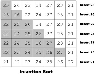
Figure 3.2: Insertion sort algorithm
The insertion sort algorithm can be coded in Python as follows:
def insertion_sort(elements):
    for i in range(1, len(elements)):
        j = i - 1
        next_element = elements[i]
        # Iterate backward through the sorted portion,
        # looking for the appropriate position for 'next_element'
        while j >= 0 and elements[j] > next_element:
            elements[j + 1] = elements[j]
            j -= 1
        elements[j + 1] = next_element
    return elements
list = [25,21,22,24,23,27,26]
insertion_sort(list)
[21, 22, 23, 24, 25, 26, 27]
In the core loop of the algorithm, we traverse through each element of the list starting from the second element (indexed at 1). For each element, the algorithm checks the preceding elements to find their correct position in the sorted sublist. This check is performed in the condition elements[j] > next_element, ensuring that we’re placing our current ‘next_element' in the appropriate position in the sorted portion of the list.
Let’s look at the performance of the insertion sort algorithm.
Performance analysis of the insertion sort algorithm
Understanding the efficiency of an algorithm is crucial in determining its suitability for different applications. Let’s delve into the performance characteristics of the insertion sort.
Best case scenario
When the input data is already sorted, insertion sort demonstrates its best behavior. In such cases, the algorithm efficiently runs in linear time, denoted as O(n), where n represents the number of elements in the data structure.
Worst case scenario
The efficiency takes a hit when the input is in reverse order, meaning the largest element is at the beginning. Here, for every element i (where i stands for the current element’s index in the loop), the inner loop might need to shift almost all preceding elements. The performance of insertion sort in this scenario can be represented mathematically by a quadratic function of the form:
where:
- w is a weighting factor, adjusting the effect of i2.
- N represents a coefficient that scales with the size of the input.
 is a constant, typically representing minor overheads not covered by the other terms.
Average case scenario
Generally, the average performance of insertion sort tends to be quadratic, which can be problematic for larger datasets.
Use cases and recommendations
Insertion sort is exceptionally efficient for:
- Small datasets.
- Nearly sorted datasets, where only a few elements are out of order.
However, for larger, more random datasets, algorithms with better average and worst-case performances, like merge sort or quick sort, are more suitable. Insertion sort’s quadratic time complexity makes it less scalable for substantial amounts of data.
Merge sort
Merge sort stands distinctively among sorting algorithms, like bubble sort and insertion sort, for its unique approach. Historically, it’s noteworthy that John von Neumann introduced this technique in 1940. While many sorting algorithms perform better on partially sorted data, merge sort remains unfazed; its performance remains consistent irrespective of the initial arrangement of the data. This resilience makes it the preferred choice for sorting large datasets.
Divide and conquer: the core of merge sort
Merge sort employs a divide-and-conquer strategy comprising two key phases – splitting and merging:
- Splitting phase: Unlike directly iterating over the list, this phase recursively divides the dataset into halves. This division continues until each section reaches a minimal size (for illustrative purposes, let’s say a single element). While it might seem counterintuitive to split data to such granular levels, this granularity facilitates the organized merging in the next phase.
- Merging phase: Here, the previously divided parts are systematically merged. The algorithm continually processes and combines these sections until the entire list is sorted.
Refer to Figure 3.3 for a visual representation of the merge sort algorithm.
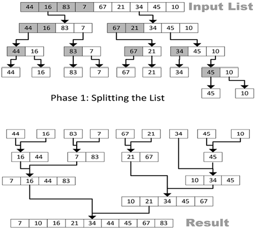
Figure 3.3: Merge sort algorithm
Pseudocode overview
Before delving into the actual code, let’s understand its logic with some pseudocode:
merge_sort (elements, start, end)
    if(start < end)
        midPoint = (end - start) / 2 + start
        merge_sort (elements, start, midPoint)
        merge_sort (elements, midPoint + 1, end)
        merge(elements, start, midPoint, end)
The pseudocode gives a snapshot of the algorithm’s steps:
- Divide the list around a central
midPoint. - Recursively split until each section has just one element.
- Systematically merge the sorted sections into a comprehensive sorted list.
Python implementation
Here’s the Python rendition of merge sort:
def merge_sort(elements):
    # Base condition to break the recursion
    if len(elements) <= 1:
        return elements
    mid = len(elements) // 2  # Split the list in half
    left = elements[:mid]
    right = elements[mid:]
    merge_sort(left)   # Sort the left half
    merge_sort(right)  # Sort the right half
    a, b, c = 0, 0, 0
    # Merge the two halves
    while a < len(left) and b < len(right):
        if left[a] < right[b]:
            elements[c] = left[a]
            a += 1
        else:
            elements[c] = right[b]
            b += 1
        c += 1
    # If there are remaining elements in the left half
    while a < len(left):
        elements[c] = left[a]
        a += 1
        c += 1
    # If there are remaining elements in the right half
    while b < len(right):
        elements[c] = right[b]
        b += 1
        c += 1
    return elements
list = [21, 22, 23, 24, 25, 26, 27]
merge_sort(list)
[21, 22, 23, 24, 25, 26, 27]
Shell sort
The bubble sort algorithm compares immediate neighbors and exchanges them if they are out of order. On the other hand, insertion sort creates the sorted list by transferring one element at a time. If we have a partially sorted list, insertion sort should give reasonable performance.
But for a totally unsorted list, sized N, you can argue that bubble sort will have to fully iterate through N-1 passes in order to get it fully sorted.
Donald Shell proposed Shell sort (named after him), which questions the importance of selecting immediate neighbors for comparison and swapping.
Now, let’s understand this concept.
In pass one, instead of selecting immediate neighbors, we use elements that are at a fixed gap, eventually sorting a sublist consisting of a pair of data points. This is shown in the following diagram. In pass two, it sorts sublists containing four data points (see the following diagram). In subsequent passes, the number of data points per sublist keeps on increasing and the number of sublists keeps on decreasing until we reach a situation where there is just one sublist that consists of all the data points.
At this point, we can assume that the list is sorted:
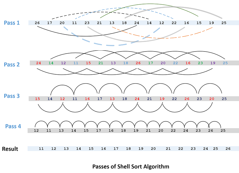
Figure 3.4: Passes in the Shell sort algorithm
In Python, the code for implementing the Shell sort algorithm is as follows:
def shell_sort(elements):
    distance = len(elements) // 2
    while distance > 0:
        for i in range(distance, len(elements)):
            temp = elements[i]
            j = i
# Sort the sub list for this distance
            while j >= distance and elements[j - distance] > temp:
                list[j] = elements[j - distance]
                j = j-distance
            list[j] = temp
# Reduce the distance for the next element
        distance = distance//2
    return elements
list = [21, 22, 23, 24, 25, 26, 27]
shell_sort(list)
[21, 22, 23, 24, 25, 26, 27]
Note that calling the ShellSort function has resulted in sorting the input array.
Performance analysis of the Shell sort algorithm
It can be observed that, in the worst case, the Shell sort algorithm will have to run through both loops giving it a complexity of O(n2). Shell sort is not for big data. It is used for medium-sized datasets. Roughly speaking, it has a reasonably good performance on a list with up to 6,000 elements. If the data is partially in the correct order, the performance will be better. In a best-case scenario, if a list is already sorted, it will only need one pass through N elements to validate the order, producing a best-case performance of O(N).
Selection sort
As we saw earlier in this chapter, bubble sort is one of the simplest sorting algorithms. Selection sort is an improvement on bubble sort, where we try to minimize the total number of swaps required with the algorithm. It is designed to make one swap for each pass, compared to N-1 passes with the bubble sort algorithm. Instead of bubbling the largest value toward the top in baby steps (as done in bubble sort, resulting in N-1 swaps), we look for the largest value in each pass and move it toward the top. So, after the first pass, the largest value will be at the top. After the second pass, the second largest value will be next to the top value. As the algorithm progresses, the subsequent values will move to their correct place based on their values.
The last value will be moved after the (N-1)th pass. So, selection sort takes N-1 passes to sort N items:
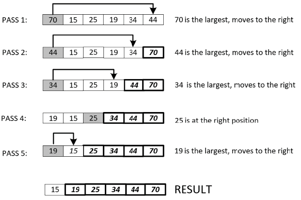
Figure 3.5: Selection sort algorithm
The implementation of selection sort in Python is shown here:
def selection_sort(list):
    for fill_slot in range(len(list) - 1, 0, -1):
        max_index = 0
        for location in range(1, fill_slot + 1):
            if list[location] > list[max_index]:
                max_index = location
        list[fill_slot],list[max_index] = list[max_index],list[fill_slot]
    return list
list = [21, 22, 23, 24, 25, 26, 27]
selection_sort(list)
[21, 22, 23, 24, 25, 26, 27]
Performance analysis of the selection sort algorithm
Selection sort’s worst-case performance is O(N2). Note that its worst performance is similar to bubble sort, and it should not be used for sorting larger datasets. Still, selection sort is a better-designed algorithm than bubble sort and its average performance is better than bubble sort due to the reduction in the number of exchanges.
Choosing a sorting algorithm
When it comes to sorting algorithms, there isn’t a one-size-fits-all solution. The optimal choice often hinges on the specific circumstances surrounding your data, such as its size and current state. Here, we’ll delve into how to make an informed decision and highlight some real-world examples.
Small and already sorted lists
For petite datasets, especially those already in order, it’s usually overkill to deploy a sophisticated algorithm. While an algorithm like merge sort is undeniably powerful, its complexities might overshadow its benefits for small data.
Real-life example: Imagine sorting a handful of books on a shelf by their authors’ last names. It’s simpler and quicker to just scan through and rearrange them manually (akin to a bubble sort) than to employ a detailed sorting method.
Partially sorted data
When dealing with data that’s already somewhat organized, algorithms like insertion sort shine. They capitalize on the existing order, enhancing efficiency.
Real-life example: Consider a classroom scenario. If students line up by height but a few are slightly out of place, the teacher can easily spot and adjust these minor discrepancies (mimicking insertion sort), rather than reordering the entire line.
Large datasets
For extensive data, where the sheer volume can be overwhelming, merge sort proves to be a reliable ally. Its divide-and-conquer strategy efficiently tackles big lists, making it an industry favorite.
Real-life example: Think about a massive library that receives thousands of books. Sorting these by publication date or author necessitates a systematic approach. Here, a method like merge sort, which breaks down the task into manageable chunks, is invaluable.
Introduction to searching algorithms
At the heart of many computational tasks lies a fundamental need: locating specific data within complex structures. On the surface, the most straightforward approach might be to scan every single data point until you find your target. But, as we can imagine, this method loses its sheen as the volume of data swells.
Why is searching so critical? Whether it’s a user querying a database, a system accessing files, or an application fetching specific data, efficient searching determines the speed and responsiveness of these operations. Without adept searching techniques, systems can become sluggish, especially with burgeoning datasets.
As the need for fast data retrieval rises, the role of sophisticated search algorithms becomes undeniable. They provide the agility and efficiency needed to wade through vast amounts of data, ensuring that systems remain nimble and users are satisfied. Thus, search algorithms act as the navigators of the digital realm, guiding us to the precise data we seek amid a sea of information.
The following searching algorithms are presented in this section:
- Linear search
- Binary search
- Interpolation search
Let’s look at each of them in more detail.
Linear search
One of the simplest strategies for searching data is to simply loop through each element looking for the target. Each data point is searched for a match and, when a match is found, the results are returned and the algorithm exits the loop. Otherwise, the algorithm keeps on searching until it reaches the end of the data. The obvious disadvantage of linear search is that it is very slow due to the inherent exhaustive search. The advantage is that the data does not need to be sorted, as required by the other algorithms presented in this chapter.
Let’s look at the code for linear search:
def linear_search(elements, item):
    index = 0
    found = False
# Match the value with each data element
    while index < len(elements) and found is False:
        if elements[index] == item:
            found = True
        else:
            index = index + 1
    return found
Let’s now look at the output of the preceding code:
list = [12, 33, 11, 99, 22, 55, 90]
print(linear_search(list, 12))
print(linear_search(list, 91))
True
False
Note that running the LinearSearch function returns a True value if it can successfully find the data.
Performance analysis of the linear search algorithm
As discussed, linear search is a simple algorithm that performs an exhaustive search. Its worst-case behavior is O(N). More info can be found at https://wiki.python.org/moin/TimeComplexity.
Binary search
The prerequisite of the binary search algorithm is sorted data. The algorithm iteratively divides a list into two parts and keeps track of the lowest and highest indices until it finds the value it is looking for:
def binary_search(elements, item):
    first = 0
    last = len(elements) - 1
    while first<=last:
        midpoint = (first + last) // 2
        if elements[midpoint] == item:
            return True
        else:
            if item < elements[midpoint]:
                last = midpoint - 1
            else:
                first = midpoint + 1
    return False
list = [12, 33, 11, 99, 22, 55, 90]
sorted_list = bubble_sort(list)
print(binary_search(list, 12))
print(binary_search(list, 91))
True
False
Note that calling the BinarySearch function will return True if the value is found in the input list.
Performance analysis of the binary search algorithm
Binary search is so named because, at each iteration, the algorithm divides the data into two parts. If the data has N items, it will take a maximum of O(logN) steps to iterate. This means that the algorithm has an O(logN) runtime.
Interpolation search
Binary search is based on the logic that it focuses on the middle section of the data. Interpolation search is more sophisticated. It uses the target value to estimate the position of the element in the sorted array. Let’s try to understand it by using an example. Let’s assume we want to search for a word in an English dictionary, such as the word river. We will use this information to interpolate and start searching for words starting with r. A more generalized interpolation search can be programmed as follows:
def int_polsearch(list,x ):
    idx0 = 0
    idxn = (len(list) - 1)
    while idx0 <= idxn and x >= list[idx0] and x <= list[idxn]:
# Find the mid point
        mid = idx0 +int(((float(idxn - idx0)/(list[idxn] - list[idx0])) * (x - list[idx0])))
# Compare the value at mid point with search value
        if list[mid] == x:
            return True
        if list[mid] < x:
            idx0 = mid + 1
    return False
list = [12, 33, 11, 99, 22, 55, 90]
sorted_list = bubble_sort(list)
print(int_polsearch(list, 12))
print(int_polsearch(list, 91))
True
False
Note that before using IntPolsearch, the array first needs to be sorted using a sorting algorithm.
Performance analysis of the interpolation search algorithm
If the data is unevenly distributed, the performance of the interpolation search algorithm will be poor. The worst-case performance of this algorithm is O(N), and if the data is somewhat reasonably uniform, the best performance is O(log(log N)).
Practical applications
The ability to efficiently and accurately search data in a given data repository is critical to many real-life applications. Depending on your choice of searching algorithm, you may need to sort the data first as well. The choice of the right sorting and searching algorithms will depend on the type and the size of the data, as well as the nature of the problem you are trying to solve.
Let’s try to use the algorithms presented in this chapter to solve the problem of matching a new applicant at the immigration department of a certain country with historical records. When someone applies for a visa to enter the country, the system tries to match the applicant with the existing historical records. If at least one match is found, then the system further calculates the number of times that the individual has been approved or refused in the past. On the other hand, if no match is found, the system classes the applicant as a new applicant and issues them a new identifier.
The ability to search, locate, and identify a person in the historical data is critical for the system. This information is important because if someone has applied in the past and the application is known to have been refused, then this may affect that individual’s current application in a negative way. Similarly, if someone’s application is known to have been approved in the past, this approval may increase the chances of that individual getting approval for their current application. Typically, the historical database will have millions of rows, and we will need a well-designed solution to match new applicants in the historical database.
Let’s assume that the historical table in the database looks like the following:
|
Personal ID |
Application ID |
First name |
Surname |
DOB |
Decision |
Decision date |
|
45583 |
677862 |
John |
Doe |
2000-09-19 |
Approved |
2018-08-07 |
|
54543 |
877653 |
Xman |
Xsir |
1970-03-10 |
Rejected |
2018-06-07 |
|
34332 |
344565 |
Agro |
Waka |
1973-02-15 |
Rejected |
2018-05-05 |
|
45583 |
677864 |
John |
Doe |
2000-09-19 |
Approved |
2018-03-02 |
|
22331 |
344553 |
Kal |
Sorts |
1975-01-02 |
Approved |
2018-04-15 |
In this table, the first column, Personal ID, is associated with each of the unique applicants in the historical database. If there are 30 million unique applicants in the historical database, then there will be 30 million unique personal IDs. Each personal ID identifies an applicant in the historical database system.
The second column we have is Application ID. Each application ID identifies a unique application in the system. A person may have applied more than once in the past. So, this means that, in the historical database, we will have more unique application IDs than personal IDs. John Doe will only have one personal ID but has two application IDs, as shown in the preceding table.
The preceding table only shows a sample of the historical dataset. Let’s assume that we have close to 1 million rows in our historical dataset, which contains the records of the last 10 years of applicants. New applicants are continuously arriving at the average rate of around 2 applicants per minute. For each applicant, we need to do the following:
- Issue a new application ID for the applicant.
- See if there is a match with an applicant in the historical database.
- If a match is found, use the personal ID for that applicant, as found in the historical database. We also need to determine how many times the application has been approved or refused in the historical database.
- If no match is found, then we need to issue a new personal ID for that individual.
Suppose a new person arrives with the following credentials:
First Name: JohnSurname: DoeDOB: 2000-09-19
Now, how can we design an application that can perform an efficient and cost-effective search?
One strategy for searching the new application in the database can be devised as follows:
- Sort the historical database by
DOB. - Each time a new person arrives, issue a new application ID to the applicant.
- Fetch all the records that match that date of birth. This will be the primary search.
- Out of the records that have come up as matches, perform a secondary search using the first and last name.
- If a match is found, use
Personal IDto refer to the applicants. Calculate the number of approvals and refusals. - If no match is found, issue a new personal ID to the applicant.
Let’s try choosing the right algorithm to sort the historical database. We can safely rule out bubble sort as the size of the data is huge. Shell sort will perform better, but only if we have partially sorted lists. So, merge sort may be the best option for sorting the historical database.
When a new person arrives, we need to search for and locate that person in the historical database. As the data is already sorted, either interpolation search or binary search can be used. Because applicants are likely to be equally spread out, as per DOB, we can safely use binary search.
Initially, we search based on DOB, which returns a set of applicants sharing the same date of birth. Now, we need to find the required person within the small subset of people who share the same date of birth. As we have successfully reduced the data to a small subset, any of the search algorithms, including bubble sort, can be used to search for the applicant. Note that we have simplified the secondary search problem here a bit. We also need to calculate the total number of approvals and refusals by aggregating the search results, if more than one match is found.
In a real-world scenario, each individual needs to be identified in the secondary search using some fuzzy search algorithm, as the first and last names may be spelled slightly differently. The search may need to use some kind of distance algorithm to implement the fuzzy search, where the data points whose similarity is above a defined threshold are considered the same.
Summary
In this chapter, we presented a set of sorting and searching algorithms. We also discussed the strengths and weaknesses of different sorting and searching algorithms. We quantified the performance of these algorithms and learned when to use each algorithm.
In the next chapter, we will study dynamic algorithms. We will also look at a practical example of designing an algorithm and the details of the page ranking algorithm. Finally, we will study the linear programming algorithm.
Learn more on Discord
To join the Discord community for this book – where you can share feedback, ask questions to the author, and learn about new releases – follow the QR code below: