
4
Designing Algorithms
This chapter presents the core design concepts of various algorithms. It discusses the strengths and weaknesses of various techniques for designing algorithms. By understanding these concepts, we will learn how to design efficient algorithms.
This chapter starts by discussing the different choices available to us when designing algorithms. Then, it discusses the importance of characterizing the particular problem that we are trying to solve. Next, it uses the famous Traveling Salesperson Problem (TSP) as a use case and applies the different design techniques that we will be presenting. Then, it introduces linear programming and discusses its applications. Finally, it presents how linear programming can be used to solve a real-world problem.
By the end of this chapter, you should be able to understand the basic concepts of designing an efficient algorithm.
The following concepts are discussed in this chapter:
- The various approaches to designing an algorithm
- Understanding the trade-offs involved in choosing the correct design for an algorithm
- Best practices for formulating a real-world problem
- Solving a real-world optimization problem
Let’s first look at the basic concepts of designing an algorithm.
Introducing the basic concepts of designing an algorithm
An algorithm, according to the American Heritage Dictionary, is defined as follows:
A finite set of unambiguous instructions that given some set of initial conditions can be performed in a prescribed sequence to achieve a certain goal and that has a recognizable set of end conditions.
Designing an algorithm is about coming up with this “finite set of unambiguous instructions” in the most efficient way to “achieve a certain goal.” For a complex real-world problem, designing an algorithm is a tedious task. To come up with a good design, we first need to fully understand the problem we are trying to solve. We start by figuring out what needs to be done (that is, understanding the requirements) before looking into how it will be done (that is, designing the algorithm). Understanding the problem includes addressing both the functional and non-functional requirements of the problem. Let’s look at what these are:
- Functional requirements formally specify the input and output interfaces of the problem that we want to solve and the functions associated with them. Functional requirements help us understand data processing, data manipulation, and the calculations that need to be implemented to generate the result.
- Non-functional requirements set the expectations about the performance and security aspects of the algorithm.
Note that designing an algorithm is about addressing both the functional and non-functional requirements in the best possible way under the given set of circumstances and keeping in mind the set of resources available to run the designed algorithm.
To come up with a good response that can meet the functional and non-functional requirements, our design should respect the following three concerns, as discussed in Chapter 1, Overview of Algorithms:
- Correctness: Will the designed algorithm produce the result we expect?
- Performance: Is this the optimal way to get these results?
- Scalability: How is the algorithm going to perform on larger datasets?
In this section, let’s look at these concerns one by one.
Concern 1: correctness: will the designed algorithm produce the result we expect?
An algorithm is a mathematical solution to a real-world problem. To be useful, it should produce accurate results. How to verify the correctness of an algorithm should not be an afterthought; instead, it should be baked into the design of the algorithm. Before strategizing how to verify an algorithm, we need to think about the following two aspects:
- Defining the truth: To verify the algorithm, we need some known correct results for a given set of inputs. These known correct results are called the truths, in the context of the problem we are trying to solve. The truth is important as it is used as a reference when we iteratively work on evolving our algorithm toward a better solution.
- Choosing metrics: We also need to think about how we are going to quantify the deviation from the defined truth. Choosing the correct metrics will help us to accurately quantify the quality of our algorithm.
For example, for supervised machine learning algorithms, we can use existing labeled data as the truth. We can choose one or more metrics, such as accuracy, recall, or precision, to quantify deviation from the truth. It is important to note that, in some use cases, the correct output is not a single value. Instead, the correct output is defined as the range for a given set of inputs. As we work on the design and development of our algorithm, the objective will be to iteratively improve the algorithm until it is within the range specified in the requirements.
- Consideration of edge cases: An edge case happens when our designed algorithm is operating at the extremes of operating parameters. An edge case is usually a scenario that is rare but needs to be well tested, as it can cause our algorithm to fail. The non-edge cases are called the “happy path” covering all the scenarios that usually happen when the operating parameters are within the normal range. The vast majority of the time, the algorithm will remain on the “happy path.” Unfortunately, there is no way to come up with all possible edge cases for a given algorithm, but we should consider as many edge cases as possible. But without consideration and thinking about the edge cases, problems may arise.
Concern 2: performance: is this the optimal way to get these results?
The second concern is about finding the answer to the following question:
Is this the optimal solution and can we verify that no other solution exists for this problem that is better than our solution?
At first glance, this question looks quite simple to answer. However, for a certain class of algorithms, researchers have unsuccessfully spent decades verifying whether a particular solution generated by an algorithm is also the best and that no other solution exists that can give better performance. So, it becomes important that we first understand the problem, its requirements, and the resources available to run the algorithm.
To provide the best solution to a certain complex problem, we need to answer the fundamental question of whether we should even aim to find the optimal solution for this problem. If finding and verifying the optimal solution is a hugely time-consuming and complex task, then a workable solution may be our best bet. These approximate workable solutions are heuristics.
So, understanding the problem and its complexities is important and helps us estimate the resource requirements.
Before we start looking deeper into this, first, let’s define a couple of terms here:
- Polynomial algorithm: If an algorithm has a time complexity of O(nk), we call it a polynomial algorithm, where k is a constant.
- Certificate: A proposed candidate solution produced at the end of an iteration is called a certificate. As we progress iteratively in solving a particular problem, we typically generate a series of certificates. If the solution is moving toward convergence, each generated certificate will be better than the previous one. At some point, when our certificate meets the requirements, we will choose that certificate as the final solution.
In Chapter 1, Overview of Algorithms, we introduced Big O notation, which can be used to analyze the time complexity of an algorithm. In the context of analyzing time complexity, we are looking at the following different time intervals:
- Candidate solution generation time, tr: It is the time it takes for an algorithm to produce a candidate solution.
- Candidate solution verification time, ts: It is the time it takes to verify the candidate solution (certificate).
Characterizing the complexity of the problem
Over the years, the research community has divided problems into various categories according to their complexity.
Before we attempt to design the solution to a problem, it makes sense to first try to characterize it. Generally, there are three types of problems:
- Problems for which we can guarantee that a polynomial algorithm exists that can be used to solve them
- Problems for which we can prove that they cannot be solved by a polynomial algorithm
- Problems for which we are unable to find a polynomial algorithm to solve them, but we are also unable to prove that a polynomial solution for those problems is impossible to find
Let’s look at the various classes of problems according to their complexity:
- Non-Deterministic Polynomial (NP): Problems that can be solved in polynomial time by a non-deterministic computer. Broadly, it means that a reasonable solution to a problem can be found and verified in polynomial times by making a reasonable guess at every step without an effort to find the optimal solution. Formally, for a problem to be an NP problem, it must meet the following condition, named Condition A:
- Condition A: It is guaranteed that there is a polynomial algorithm that can be used to verify that the candidate solution (certificate) is optimal.
- Polynominal (P): Problems that can be solved in polynomial time by a deterministic computer. These problems can be solved by some algorithm with runtime O(Nk) for some power k, no matter how large. These are types of problems that can be thought of as a subset of NP. In addition to meeting the condition of an NP problem, Condition A, P problems need to meet another condition, named Condition B:
- Condition A: It is guaranteed that there is a polynomial algorithm that can be used to verify that the candidate solution (certificate) is optimal.
- Condition B: It is guaranteed that there is at least one polynomial algorithm that can be used to solve them.
Exploring the relationship between P and NP
Understanding the relationship between P and NP is still a work in progress. What we know for sure is that P is a subset of NP, i.e., ![]() . That is obvious from the above discussion where NP needs to meet only the first of the two conditions that P needs to meet.
. That is obvious from the above discussion where NP needs to meet only the first of the two conditions that P needs to meet.
The relationship between P and NP problems is shown in Figure 4.1:
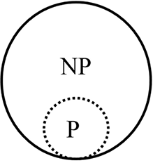
Figure 4.1: Relationship between P and NP problems
What we do not know for sure is that if a problem is NP, is it P as well? This is one of the greatest problems in computer science that remains unresolved. Millennium Prize Problems, selected by the Clay Mathematics Institute, has announced a 1-million-dollar prize for the solution to this problem as it will have a major impact on fields such as AI, cryptography, and theoretical computer sciences. There are certain problems, such as sorting, that are known to be in P. Others, such as the knapsack and TSP, are known to be in NP.
There is a lot of ongoing research effort to answer this question. As yet, no researcher has discovered a polynomial-time-deterministic algorithm to solve the knapsack or TSP. It is still a work in progress and no one has been able to prove that no such algorithm is possible.
Figure 4.2: DoesP = NP? We do not know as yet
Introducing NP-complete and NP-hard
Let’s continue the list of various classes of problems:
- NP-complete: The NP-complete category contains the hardest problems of all NP problems. An NP-complete problem meets the following two conditions:
- There are no known polynomial algorithms to generate a certificate.
- There are known polynomial algorithms to verify that the proposed certificate is optimal.
- NP-hard: The NP-hard category contains problems that are at least as hard as any problem in the NP category, but that do not themselves need to be in the NP category.
Now, let’s try to draw a diagram to illustrate these different classes of problems:
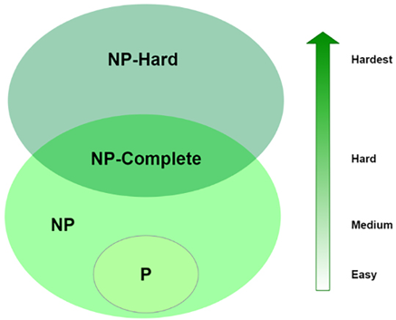
Figure 4.3: Relationship between P, NP, NP-complete, and NP-hard
Note that it is still to be proven by the research community whether P = NP. Although this has not yet been proven, it is extremely likely that P ≠ NP. In that case, no polynomial solution exists for NP-complete problems. Note that the preceding diagram is based on this assumption.
The distinction between P, NP, NP-complete, and NP-hard
Unfortunately, the distinction between P, NP, NP-compete, and NP-hard is not clear-cut. Let us summarize and study some examples to make better sense of the concepts discussed in this section:
- P: It is the class of problems solvable in polynomial time. For example:
- Hashtable lookup
- Shortest path algorithms like Djikstra’s algorithms
- Linear and binary search algorithms
- NP-problem: The problems are not solvable in polynomial time, but their solution can be verified in polynomial time. For example:
- RSA encryption algorithm
- NP-hard: These are complex problems that no one has come up with a solution for as yet, but if solved, would have a polynomial time solution. For example:
- Optimal clustering using the K-means algorithm
- NP-complete: The NP-complete problems are the “hardest” in NP. They are both NP-hard and NP. For example:
Finding a solution for one of either classes (NP-hard or NP-complete) would imply a solution for all NP-hard/NP-complete problems.
Concern 3 – scalability: how is the algorithm going to perform on larger datasets?
An algorithm processes data in a defined way to produce a result. Generally, as the size of the data increases, it takes more and more time to process the data and calculate the required results. The term big data is sometimes used to roughly identify datasets that are expected to be challenging for the infrastructure and algorithms to work with due to their volume, variety, and velocity. A well-designed algorithm should be scalable, which means that it should be designed in a way that means, wherever possible, it should be able to run efficiently, making use of the available resources and generating the correct results in a reasonable timeframe. The design of the algorithm becomes even more important when dealing with big data. To quantify the scalability of an algorithm, we need to keep the following two aspects in mind:
- The increase in resource requirements as the input data is increased: Estimating a requirement such as this is called space complexity analysis.
- The increase in the time taken to run as the input data is increased: Estimating this is called time complexity analysis.
Note that we are living in an era that is defined by data explosion. The term big data has become mainstream, as it captures the size and complexity of the data that is typically required to be processed by modern algorithms.
While in the development and testing phase, many algorithms use only a small sample of data. When designing an algorithm, it is important to look into the scalability aspect of the algorithms. In particular, it is important to carefully analyze (that is, test or predict) the effect of an algorithm’s performance as datasets increase in size.
The elasticity of the cloud and algorithmic scalability
Cloud computing has made new options available to deal with the resource requirements of an algorithm. Cloud computing infrastructures are capable of provisioning more resources as the processing requirements increase. The ability of cloud computing is called the elasticity of the infrastructure and has now provided us with more options for designing an algorithm. When deployed on the cloud, an algorithm may demand additional CPUs or VMs based on the size of the data to be processed.
Typical deep learning algorithms are a good example. To train a good deep learning model, lots of labeled data is needed. For a well-designed deep learning algorithm, the processing required to train a deep learning model is directly proportional to the number of examples or close to it. When training a deep learning model in the cloud, as the size of data increases, we try to provision more resources to keep training time within manageable limits.
Understanding algorithmic strategies
A well-designed algorithm tries to optimize the use of the available resources most efficiently by dividing the problem into smaller subproblems wherever possible. There are different algorithmic strategies for designing algorithms. An algorithmic strategy deals with the following three aspects of an algorithm list containing aspects of the missing algorithm.
We will present the following three strategies in this section:
- The divide-and-conquer strategy
- The dynamic programming strategy
- The greedy algorithm strategy
Understanding the divide-and-conquer strategy
One of the strategies is to find a way to divide a larger problem into smaller problems that can be solved independently of each other. The subsolutions produced by these subproblems are then combined to generate the overall solution to the problem. This is called the divide-and-conquer strategy.
Mathematically, if we are designing a solution for a problem (P) with n inputs that needs to process dataset d, we split the problem into k subproblems, P1 to Pk. Each of the subproblems will process a partition of the dataset, d. Typically, we will have P1 to Pk processing d1 to dk respectively.
Let’s look at a practical example.
A practical example – divide-and-conquer applied to Apache Spark
Apache Spark (https://spark.apache.org/) is an open-source framework that is used to solve complex distributed problems. It implements a divide-and-conquer strategy to solve problems. To process a problem, it divides the problem into various subproblems and processes them independently of each other. These subproblems can run on separate machines enabling horizontal scaling. We will demonstrate this by using a simple example of counting words from a list.
Let’s assume that we have the following list of words:
words_list = ["python", "java", "ottawa", "news", "java", "ottawa"]
We want to calculate the frequency of each word in this list. For that, we will apply the divide-and-conquer strategy to solve this problem in an efficient way.
The implementation of divide-and-conquer is shown in the following diagram:
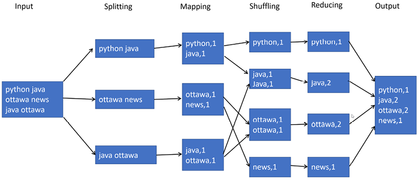
The preceding diagram shows the following phases into which a problem is divided:
- Splitting: The input data is divided into partitions that can be processed independently of each other. This is called splitting. We have three splits in the preceding figure.
- Mapping: Any operation that can run independently on a split is called a map. In the preceding diagram, the map operation converts each of the words in the partition in to key-value pairs. Corresponding to the three splits, there are three mappers that are run in parallel.
- Shuffling: Shuffling is the process of bringing similar keys together. Once similar keys are brought together, aggregation functions can be run on their values. Note that shuffling is a performance-intensive operation, as similar keys need to be brought together that can be originally distributed across the network.
- Reducing: Running an aggregation function on the values of similar keys is called reducing. In the preceding diagram, we have to count the number of words.
Let’s see how we can write the code to implement this. To demonstrate the divide-and-conquer strategy, we need a distributed computing framework. We will run Python running on Apache Spark for this:
- First, in order to use Apache Spark, we will create a runtime context of Apache Spark:
import findspark findspark.init() from pyspark.sql import SparkSession spark = SparkSession.builder.master("local[*]").getOrCreate() sc = spark.sparkContext - Now, let’s create a sample list containing some words. We will convert this list into Spark’s native distributed data structure, called a Resilient Distributed Dataset (RDD):
wordsList = ['python', 'java', 'ottawa', 'ottawa', 'java','news'] wordsRDD = sc.parallelize(wordsList, 4) # Print out the type of wordsRDD print (wordsRDD.collect()) - It will print:
['python', 'java', 'ottawa', 'ottawa', 'java', 'news'] - Now, let’s use a
mapfunction to convert the words into a key-value pair:wordPairs = wordsRDD.map(lambda w: (w, 1)) print (wordPairs.collect()) - It will print:
[('python', 1), ('java', 1), ('ottawa', 1), ('ottawa', 1), ('java', 1), ('news', 1)] - Let’s use the
reducefunction to aggregate and get the result:wordCountsCollected = wordPairs.reduceByKey(lambda x,y: x+y) print(wordCountsCollected.collect()) - It prints:
[('python', 1), ('java', 2), ('ottawa', 2), ('news', 1)]
This shows how we can use the divide-and-conquer strategy to count the number of words. Note that divide-and-conquer is useful when a problem can be divided into subproblems and each subproblem can at least be partially solved independently of other subproblems. It is not the best choice for algorithms that require intensive iterative processing, such as optimization algorithms. For such algorithms, dynamic programming is suitable, which is presented in the next section.
Modern cloud computing infrastructures, such as Microsoft Azure, Amazon Web Services, and Google Cloud, achieve scalability in a distributed infrastructure that uses several CPUs/GPUs in parallel by implementing a divide-and-conquer strategy either directly or indirectly behind the scenes.
Understanding the dynamic programming strategy
In the previous section, we studied divide and conquer, which is a top-down method. In contrast, dynamic programming is a bottom-up strategy. We start with the smallest subproblem and keep on combining the solutions. We keep on combining until we reach the final solution. Dynamic programming, like the divide-and-conquer method, solves problems by combining the solutions with subproblems.
Dynamic programming is a strategy proposed in the 1950s by Richard Bellman to optimize certain classes of algorithms. Note that in dynamic programming, the word “programming” refers to the use of a tabular method and has nothing to do with writing code. In contrast to the divide and conquer strategy, dynamic programming is applicable when the subproblems are not independent. It is typically applied to optimization problems in which each subproblem’s solution has a value.
Our objective is to find a solution with optimal value. A dynamic programming algorithm solves every subproblem just once and then saves its answer in a table, thereby avoiding the work of recomputing the answer every time the subproblem is encountered.
Components of dynamic programming
Dynamic programming is based on two major components:
- Recursion: It solves subproblems recursively.
- Memoization: Memoization or caching. It is based on an intelligent caching mechanism that tries to reuse the results of heavy computations. This intelligent caching mechanism is called memoization. The subproblems partly involve a calculation that is repeated in those subproblems. The idea is to perform that calculation once (which is the time-consuming step) and then reuse it on the other subproblems. This is achieved using memoization, which is especially useful in solving recursive problems that may evaluate the same inputs multiple times.
Conditions for using dynamic programming
The problem we are trying to solve with dynamic programming should have two characteristics.
- Optimal structure: Dynamic programming gives good performance benefits when the problem we are trying to solve can be divided into subproblems.
- Overlapping subproblems: Dynamic programming uses a recursive function that solves a particular problem by calling a copy of itself and solving smaller subproblems of the original problems. The computed solutions of the subproblems are stored in a table, so that these don’t have to be re-computed. Hence, this technique is needed where an overlapping sub-problem exists.
Dynamic programming is a perfect fit for combinatorial optimization problems, which are problems that needs providing optimal combinations of input elements as a solution.
Examples include:
- Finding the optimal way to deliver packages for a company like FedEx or UPS
- Finding the optimal airline routes and airports
- Deciding how to assign drivers for an online food delivery system like Uber Eats
Understanding greedy algorithms
As the name indicates, a greedy algorithm relatively quickly produces a good solution, but it cannot be the optimal solution. Like dynamic programming, greedy algorithms are mainly used to solve optimization problems where a divide-and-conquer strategy cannot be used. In the greedy algorithm, the solution is calculated following a sequence of steps. At each step, a locally optimal choice is made.
Conditions for using greedy programming
Greedy is a strategy that works well on problems with the following two characteristics:
- Global from local: A global optimum can be arrived at by selecting a local optimum.
- Optimal substructure: An optimal solution to the problem is made from optimal solutions to subproblems.
To understand the greedy algorithm, let’s first define two terms:
- Algorithmic overheads: Whenever we try to find the optimal solution to a certain problem, it takes some time. As the problems that we are trying to optimize become more and more complex, the time it takes to find the optimal solution also increases. We represent algorithmic overheads with
 .
. - Delta from optimal: For a given optimization problem, there exists an optimal solution. Typically, we iteratively optimize the solution using our chosen algorithm. For a given problem, there always exists a perfect solution, called the optimal solution, to the current problem. As discussed, based on the classification of the problem we are trying to solve, it’s possible for the optimal solution to be unknown or for it to take an unreasonable amount of time to calculate and verify it. Assuming that the optimal solution is known, the difference from optimal for the current solution in the ith iteration is called delta from optimal and is represented by
 .
.
For complex problems, we have two possible strategies:
- Spend more time finding a solution nearest to optimal so that
 is as small as possible.
 - Minimize the algorithmic overhead,
 . Use the quick-and-dirty approach and just use a workable solution.
Greedy algorithms are based on the second strategy, where we do not make an effort to find a global optimal and choose to minimize the algorithm overheads instead.
Using a greedy algorithm is a quick and simple strategy for finding the global optimal value for multistage problems. It is based on selecting the local optimal values without making an effort to verify whether local optimal values are globally optimal as well. Generally, unless we are lucky, a greedy algorithm will not result in a value that can be considered globally optimal. However, finding a global optimal value is a time-consuming task. Hence, the greedy algorithm is fast compared to the divide-and-conquer and dynamic programming algorithms.
Generally, a greedy algorithm is defined as follows:
- Let’s assume that we have a dataset, D. In this dataset, choose an element, k.
- Let’s assume the candidate solution or certificate is S. Consider including k in the solution, S. If it can be included, then the solution is Union(S, e).
- Repeat the process until S is filled up or D is exhausted.
Example:
The Classification And Regression Tree (CART) algorithm is a greedy algorithm, which searches for an optimum split at the top level. It repeats the process at each subsequent level. Note that the CART algorithm does not calculate and check whether the split will lead to the lowest possible impurity several levels down. CART uses a greedy algorithm because finding the optimal tree is known to be an NP-complete problem. It has an algorithmic complexity of O(exp(m)) time.
A practical application – solving the TSP
Let’s first look at the problem statement for the TSP, which is a well-known problem that was coined as a challenge in the 1930s. The TSP is an NP-hard problem. To start with, we can randomly generate a tour that meets the condition of visiting all of the cities without caring about the optimal solution. Then, we can work to improve the solution with each iteration. Each tour generated in an iteration is called a candidate solution (also called a certificate). Proving that a certificate is optimal requires an exponentially increasing amount of time. Instead, different heuristics-based solutions are used that generate tours that are near to optimal but are not optimal.
A traveling salesperson needs to visit a given list of cities to get their job done:
|
INPUT |
A list of n cities (denoted as V) and the distances between each pair of cities, d ij (1 ≤ i, j ≤ n) |
|
OUTPUT |
The shortest tour that visits each city exactly once and returns to the initial city |
Note the following:
- The distances between the cities on the list are known
- Each city in the given list needs to be visited exactly once
Can we generate the travel plan for the salesperson? What will be the optimal solution that can minimize the total distance traveled by the traveling salesperson?
The following are the distances between five Canadian cities that we can use for the TSP:
|
Ottawa |
Montreal |
Kingston |
Toronto |
Sudbury | |
|
Ottawa |
- |
199 |
196 |
450 |
484 |
|
Montreal |
199 |
- |
287 |
542 |
680 |
|
Kingston |
196 |
287 |
- |
263 |
634 |
|
Toronto |
450 |
542 |
263 |
- |
400 |
|
Sudbury |
484 |
680 |
634 |
400 |
- |
Note that the objective is to get a tour that starts and ends in the initial city. For example, a typical tour can be Ottawa–Sudbury–Montreal–Kingston–Toronto–Ottawa with a cost of 484 + 680 + 287 + 263 + 450 = 2,164. Is this the tour in which the salesperson has to travel the minimum distance? What will be the optimal solution that can minimize the total distance traveled by the traveling salesperson? I will leave this up to you to think about and calculate.
Using a brute-force strategy
The first solution that comes to mind to solve the TSP is using brute force to come up with the shortest path in which the salesperson visits every city exactly once and returns to the initial city. So, the brute-force strategy works as follows:
- Evaluate all possible tours.
- Choose the one for which we get the shortest distance.
The problem is that for n number of cities, there are (n-1)! possible tours. That means that five cities will produce 4! = 24 tours, and we will select the one that corresponds to the lowest distance. It is obvious that this method will only work when we do not have too many cities. As the number of cities increases, the brute-force strategy becomes unsolvable due to the large number of permutations generated by using this approach.
Let’s see how we can implement the brute-force strategy in Python.
First, note that a tour, {1,2,3}, represents a tour of the city from city 1 to city 2 and city 3. The total distance in a tour is the total distance covered in a tour. We will assume that the distance between the cities is the shortest distance between them (which is the Euclidean distance).
Let’s first define three utility functions:
distance_points: Calculates the absolute distance between two pointsdistance_tour: Calculates the total distance the salesperson has to cover in a given tourgenerate_cities: Randomly generates a set of n cities located in a rectangle of width500and height300
Let’s look at the following code:
import random
from itertools import permutations
In the preceding code, we implemented alltours from the permutations function of the itertools package. We have also represented the distance with a complex number. This means the following:
Calculating the distance between two cities, a and b, is as simple as distance (a,b).
We can create n number of cities just by calling generate_cities(n):
def distance_tour(aTour):
    return sum(distance_points(aTour[i - 1], aTour[i])
               for i in range(len(aTour))
    )
aCity = complex
def distance_points(first, second):
    return abs(first - second)
def generate_cities (number_of_cities):
    seed=111
    width=500
    height=300
    random.seed((number_of_cities, seed))
    return frozenset(aCity(random.randint(1, width),
                           random.randint(1, height))
                     for c in range(number_of_cities))
Now let’s define a function, brute_force, that generates all the possible tours of the cities. Once it has generated all possible tours, it will choose the one with the shortest distance:
def brute_force(cities):
    return shortest_tour(alltours(cities))
def shortest_tour(tours):
    return min(tours, key=distance_tour)
Now let’s define the utility functions that can help us plot the cities. We will define the following functions:
visualize_tour: Plots all the cities and links in a particular tour. It also highlights the city from which the tour started.visualize_segment: Used byvisualize_tourto plot cities and links in a segment.
Look at the following code:
import matplotlib.pyplot as plt
def visualize_tour(tour, style='bo-'):
if len(tour) > 1000:
        plt.figure(figsize=(15, 10))
    start = tour[0:1]
    visualize_segment(tour + start, style)
    visualize_segment(start, 'rD')

def visualize_segment (segment, style='bo-'):
    plt.plot([X(c) for c in segment], [Y(c) for c in segment], style, clip_on=False)
    plt.axis('scaled')
    plt.axis('off')

def X(city):
    "X axis";
    return city.real
def Y(city):
    "Y axis";
    return city.imag
Let’s implement a function, tsp(), that does the following:
- Generates the tour based on the algorithm and number of cities requested.
- Calculates the time it took for the algorithm to run.
- Generates a plot.
Once tsp() is defined, we can use it to create a tour:
from time import time
from collections import Counter
def tsp(algorithm, cities):
    t0 = time()
    tour = algorithm(cities)
    t1 = time()
    # Every city appears exactly once in tour
    assert Counter(tour) == Counter(cities)
    visalize_tour(tour)
    print("{}:{} cities => tour length {;.0f} (in {:.3f} sec".format(
        name(algorithm), len(tour), distance_tour(tour), t1-t0))
def name(algorithm):
    return algorithm.__name__.replace('_tsp','')
tps(brute_force, generate_cities(10))
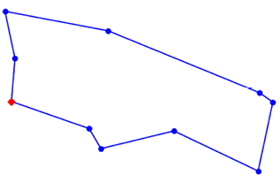
Figure 4.5: Solution of TSP
Note that we have used it to generate the tour for 10 cities. As n = 10, it will generate (10-1)! = 362,880 possible permutations. If n increases, the number of permutations sharply increases and the brute-force method cannot be used.
Using a greedy algorithm
If we use a greedy algorithm to solve the TSP, then, at each step, we can choose a city that seems reasonable, instead of finding a city to visit that will result in the best overall path. So, whenever we need to select a city, we just select the nearest city without bothering to verify that this choice will result in the globally optimal path.
The approach of the greedy algorithm is simple:
- Start from any city.
- At each step, keep building the tour by moving to the next city where the nearest neighborhood has not been visited before.
- Repeat step 2.
Let’s define a function named greedy_algorithm that can implement this logic:
def greedy_algorithm(cities, start=None):
    city_ = start or first(cities)
    tour = [city_]
    unvisited = set(cities - {city_})
    while unvisited:
        city_ = nearest_neighbor(city_, unvisited)
        tour.append(city_)
        unvisited.remove(city_)
    return tour
def first(collection): return next(iter(collection))
def nearest_neighbor(city_a, cities):
    return min(cities, key=lambda city_: distance_points(city_, city_a))
Now, let’s use greedy_algorithm to create a tour for 2,000 cities:
tsp(greedy_algorithm, generate_cities(2000))
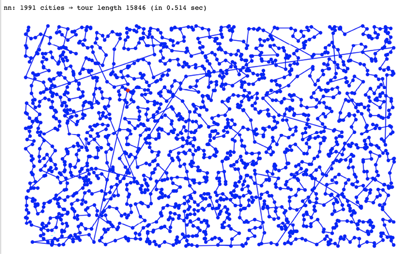
Figure 4.6: Cities displayed in Jupyter Notebook
Note that it took only 0.514 seconds to generate the tour for 2,000 cities. If we had used the brute-force method, it would have generated (2000-1)! = 1.65e5732 permutations, which is almost infinite.
Note that the greedy algorithm is based on heuristics and there is no proof that the solution will be optimal.
Comparison of Three Strategies
To summarize, the outcome of the greedy algorithm is more efficient in terms of calculation time whereas the brute-force method provides the combination with the global optimum. This means the calculation time as well as the quality of the outcome differ. The proposed greedy algorithm may reach nearly as high outcomes as brute force does, with significantly less calculation time, but as it does not search for an optimal solution, it is based on a effort-based strategy and there are no guarantees.
Now, let’s look at the design of the PageRank algorithm.
Presenting the PageRank algorithm
As a practical example, let’s look at the PageRank algorithm, which is used by Google to rank the search results of a user query. It generates a number that quantifies the importance of search results in the context of the query the user has executed. This was designed by two Ph.D. students, Larry Page and Sergey Brin, at Stanford in the late 1990s, who also went on to start Google. The PageRank algorithm was named after Larry Page.
Let’s first formally define the problem for which PageRank was initially designed.
Problem definition
Whenever a user enters a query on a search engine on the web, it typically results in a large number of results. To make the results useful for the end user, it is important to rank the web pages using some criteria. The results that are displayed use this ranking to summarize the results for the user and are dependent on the criteria defined by the underlying algorithm being used.
Implementing the PageRank algorithm
First, while using the PageRank algorithm, the following representation is used:
- Web pages are represented by nodes in a directed graph.
- The graph edges correspond to hyperlinks.
The most important part of the PageRank algorithm is to come up with the best way to calculate the importance of each page that is returned by the query results. The rank of a particular web page in the network is calculated as the probability that a person randomly traversing the edges (i.e., clicking on links) will arrive at that page. Also, this algorithm is parametrized by the damping factor alpha, which has a default value of 0.85. This damping factor is the probability that the user will continue clicking. Note that the page with the highest PageRank is the most attractive: regardless of where the person starts, this page has the highest probability of being the final destination.
The algorithm requires many iterations or passes through the collection of web pages to determine the right importance (or PageRank value) of each web page.
To calculate a number from 0 to 1 that can quantify the importance of a particular page, the algorithm incorporates information from the following two components:
- Information that was specific to the query entered by the user: This component estimates, in the context of the query entered by the user, how relevant the content of the web page is. The content of the page is directly dependent on the author of the page.
- Information that was not relevant to the query entered by the user: This component tries to quantify the importance of each web page in the context of its links, views, and neighborhood. The neighborhood of a web page is the group of web pages directly connected to a certain page. This component is difficult to calculate as web pages are heterogeneous, and coming up with criteria that can be applied across the web is difficult to develop.
In order to implement the PageRank algorithm in Python, first, let’s import the necessary libraries:
import numpy as np
import networkx as nx
import matplotlib.pyplot as plt
Note that the network is from https://networkx.org/. For the purpose of this demonstration, let’s assume that we are analyzing only five web pages in the network. Let’s call this set of pages my_pages and together they are in a network named my_web:
my_web = nx.DiGraph()
my_pages = range(1,6)
Now, let’s connect them randomly to simulate an actual network:
connections = [(1,3),(2,1),(2,3),(3,1),(3,2),(3,4),(4,5),(5,1),(5,4)]
my_web.add_nodes_from(my_pages)
my_web.add_edges_from(connections)
Now, let’s plot this graph:
pos = nx.shell_layout(my_web)
nx.draw(my_web, pos, arrows=True, with_labels=True)
plt.show()
It creates the visual representation of our network, as follows:
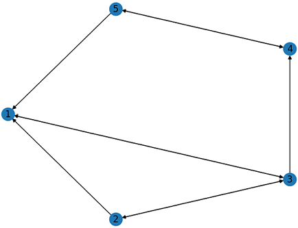
Figure 4.7: Visual representation of the network
In the PageRank algorithm, the patterns of a web page are contained in a matrix called the transition matrix. There are algorithms that constantly update the transition matrix to capture the constantly changing state of the web. The size of the transition matrix is n x n, where n is the number of nodes. The numbers in the matrix are the probability that a visitor will next go to that link due to the outbound link.
In our case, the preceding graph shows the static web that we have. Let’s define a function that can be used to create the transition matrix:
def create_page_rank(a_graph):
    nodes_set = len(a_graph)
    M = nx.to numpy_matrix(a_graph)
    outwards = np.squeeze(np.asarray (np. sum (M, axis=1)))
    prob outwards = np.array([
        1.0 / count if count>0
        else 0.0
        for count in outwards
    ])
    G = np.asarray(np.multiply (M.T, prob_outwards))
    p = np.ones(nodes_set) / float (nodes_set)
    return G, p
Note that this function will return G, which represents the transition matrix for our graph.
Let’s generate the transition matrix for our graph:
G,p = create_page_rank(my_web)
print (G)
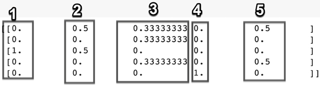
Figure 4.8: Transition matrix
Note that the transition matrix is 5 x 5 for our graph. Each column corresponds to each node in the graph. For example, column 2 is about the second node. There is a 0.5 probability that the visitor will navigate from node 2 to node 1 or node 3. Note that the diagonal of the transition matrix is 0 as in our graph, there is no outbound link from a node to itself. In an actual network, it may be possible.
Note that the transition matrix is a sparse matrix. As the number of nodes increases, most of its values will be 0. Thus, the structure of a graph is extracted as a transition matrix. In a transaction matrix, nodes are represented in columns and rows:
- Columns: Indicates to the node that a web surfer is online
- Rows: Indicates the probability that the surfer will visit other nodes because of outbound links
In the real web, the transition matrix that feeds the PageRank algorithm is built by spiders’ continuous exploration of links.
Understanding linear programming
Many real-world problems involve maximizing or minimizing an objective, with some given constraints. One approach is to specify the objective as a linear function of some variables. We also formulate the constraints on resources as equalities or inequalities on those variables. This approach is called the linear programming problem. The basic algorithm behind linear programming was developed by George Dantzig at the University of California at Berkeley in the early 1940s. Dantzig used this concept to experiment with logistical supply-and-capacity planning for troops while working for the US Air Force.
At the end of the Second World War, Dantzig started working for the Pentagon and matured his algorithm into a technique that he named linear programming. It was used for military combat planning.
Today, it is used to solve important real-world problems that relate to minimizing or maximizing a variable based on certain constraints. Some examples of these problems are as follows:
- Minimizing the time to repair a car at a mechanic shop based on the resources
- Allocating available distributed resources in a distributed computing environment to minimize response times
- Maximizing the profit of a company based on the optimal assignment of resources within the company
Formulating a linear programming problem
The conditions for using linear programming are as follows:
- We should be able to formulate the problem through a set of equations.
- The variables used in the equation must be linear.
Defining the objective function
Note that the objective of each of the preceding three examples is about minimizing or maximizing a variable. This objective is mathematically formulated as a linear function of other variables and is called the objective function. The aim of a linear programming problem is to minimize or maximize the objective function while remaining within the specified constraints.
Specifying constraints
When trying to minimize or maximize something, there are certain constraints in real-world problems that need to be respected. For example, when trying to minimize the time it takes to repair a car, we also need to consider that there is a limited number of mechanics available. Specifying each constraint through a linear equation is an important part of formulating a linear programming problem.
A practical application – capacity planning with linear programming
Let’s look at a practical use case where linear programming can be used to solve a real-world problem.
Let’s assume that we want to maximize the profits of a state-of-the-art factory that manufactures two different types of robots:
- Advanced model (A): This provides full functionality. Manufacturing each unit of the advanced model results in a profit of $4,200.
- Basic model (B): This only provides basic functionality. Manufacturing each unit of the basic model results in a profit of $2,800.
There are three different types of people needed to manufacture a robot. The exact number of days needed to manufacture a robot of each type is as follows:
|
Type of Robot |
Technician |
AI Specialist |
Engineer |
|
Robot A: advanced model |
3 days |
4 days |
4 days |
|
Robot B: basic model |
2 days |
3 days |
3 days |
The factory runs on 30-day cycles. A single AI specialist is available for 30 days in a cycle. Each of the two engineers will take 8 days off in 30 days. So, an engineer is available only for 22 days in a cycle. There is a single technician available for 20 days in a 30-day cycle.
The following table shows the number of people we have in the factory:
|
Technician |
AI Specialist |
Engineer | |
|
Number of people |
1 |
1 |
2 |
|
Total number of days in a cycle |
1 x 20 = 20 days |
1 x 30 = 30 days |
2 x 22 = 44 days |
This can be modeled as follows:
- Maximum profit = 4200A + 2800B
- This is subject to the following:
A ≥ 0: The number of advanced robots produced can be 0 or more.B ≥0: The number of basic robots produced can be 0 or more.3A + 2B ≤ 20: These are the constraints of the technician’s availability.4A+3B ≤ 30: These are the constraints of the AI specialist’s availability.4A+ 3B ≤ 44: These are the constraints of the engineers’ availability.
First, we import the Python package named pulp, which is used to implement linear programming:
import pulp
Then, we call the LpProblem function in this package to instantiate the problem class. We name the instance Profit maximising problem:
# Instantiate our problem class
model = pulp.LpProblem("Profit_maximising_problem", pulp.LpMaximize)
Then, we define two linear variables, A and B. Variable A represents the number of advanced robots that are produced and variable B represents the number of basic robots that are produced:
A = pulp.LpVariable('A', lowBound=0,  cat='Integer')
B = pulp.LpVariable('B', lowBound=0, cat='Integer')
We define the objective function and constraints as follows:
# Objective function
model += 5000 * A + 2500 * B, "Profit"
# Constraints
model += 3 * A + 2 * B <= 20
model += 4 * A + 3 * B <= 30
model += 4 * A + 3 * B <= 44
We use the solve function to generate a solution:
# Solve our problem
model.solve()
pulp.LpStatus[model.status]
Then, we print the values of A and B and the value of the objective function:
# Print our decision variable values
print (A.varValue)
print (B.varValue)
The output is:
6.0
1.0
# Print our objective function value
print (pulp.value(model.objective))
It prints:
32500.0
Linear programming is extensively used in the manufacturing industry to find the optimal number of products that should be used to optimize the use of available resources.
And here we come to the end of this chapter! Let’s summarize what we have learned.
Summary
In this chapter, we studied various approaches to designing an algorithm. We looked at the trade-offs involved in choosing the correct design of an algorithm. We looked at the best practices for formulating a real-world problem. We also learned how to solve a real-world optimization problem. The lessons learned from this chapter can be used to implement well-designed algorithms.
In the next chapter, we will focus on graph-based algorithms. We will start by looking at different ways of representing graphs. Then, we will study the techniques to establish a neighborhood around various data points to conduct a particular investigation. Finally, we will study the optimal ways to search for information in graphs.
Learn more on Discord
To join the Discord community for this book – where you can share feedback, ask questions to the author, and learn about new releases – follow the QR code below: