
Chapter 8 - OLAP Functions
“Don’t count the days, make the days count.”
– Mohammed Ali
On-Line Analytical Processing (OLAP) or Ordered Analytics

OLAP is often called Ordered Analytics because the first thing every OLAP does before any calculating is SORT all the rows. The query above sorts by Sale_Date and then does a cumulative sum on the Daily_Sales column.
Cumulative Sum (CSUM) Command and how OLAP Works
SELECT |
Product_ID , Sale_Date, Daily_Sales |
|
,CSUM(Daily_Sales, Sale_Date) AS "CSum" |
FROM |
Sales_Table ; |

OLAP always sorts the rows first. That is why they are called Ordered Analytics. They order the data first and then calculate the rows once the sort has taken place. This CSUM will calculate the first sorted row and continuing to the last sorted row, thus calculating the cumulative sum for all Daily_Sales.
After the Sort the CSUM is Calculated
SELECT |
Product_ID , Sale_Date, Daily_Sales |
|
,CSUM(Daily_Sales, Sale_Date) AS "CSum" |
FROM |
Sales_Table ; |
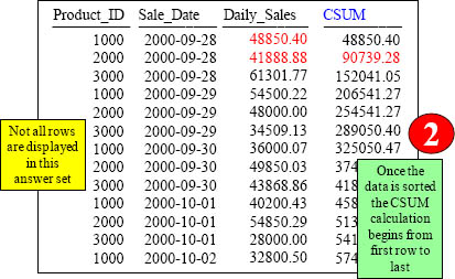
Once the data is first sorted by Sale_Date then phase 2 is ready and the OLAP calculation can be performed on the sorted data. Day 1 we made 48850.40! Add the next row’s Daily_Sales to get a Cumulative Sum (CSUM) to get 90739.28!
The OLAP Major Sort Key

In a CSUM, the second column listed is always the major SORT KEY. The SORT KEY in the above query is Sale_Date. Notice again the answer set is sorted by this. After the sort has finished the CSUM is calculated starting with the first sorted row till the end.
The OLAP Major Sort Key and the Minor Sort Key(s)

Product_ID is the MAJOR sort key and Sale_Date is the MINOR Sort key above.
Troubleshooting OLAP – My Data isn’t coming back Correct

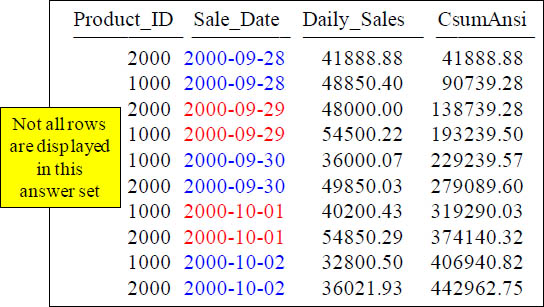
The first thing every OLAP does is SORT. That means you should NEVER put an ORDER BY at the end. It will mess up the ENTIRE result set. The data rows above are calculated correctly, but the reordering makes the data look wrong.
GROUP BY in Teradata OLAP Syntax Resets on the Group

The GROUP BY Statement cause the CSUM to start over (reset) on its calculating the cumulative sum of the Daily_Sales each time it runs into a NEW Product_ID.
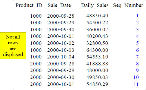
CSUM the Number 1 to get a Sequential Number
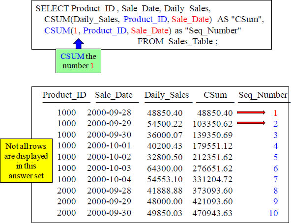
With “Seq_Number”, because you placed the number 1 in the area where it calculates, it will continuously add 1 to the answer for each row.
A Single GROUP BY Resets each OLAP with Teradata Syntax

What does the GROUP BY Statement cause? Both OLAP Commands to reset! All Teradata OLAP commands reset simultaneously with one GROUP BY statement. We will soon learn about the ANSI version, which is much better.
CSUM
This ANSI version of CSUM is SUM() Over. Right now, the syntax wants to see the sum of the Daily_Sales after it is first sorted by Sale_Date. Rows Unbounded Preceding means to start calculating from the first row, and continue calculating until the last row. This Rows Unbounded Preceding makes this a CSUM. The ANSI Syntax seems difficult, but only at first.
CSUM – The Sort Explained
SELECT Product_ID , Sale_Date, Daily_Sales,
SUM(Daily_Sales) OVER (ORDER BY Sale_Date
ROWS UNBOUNDED PRECEDING) AS CsumAnsi
FROM Sales_Table
WHERE Product_ID BETWEEN 1000 and 2000 ;
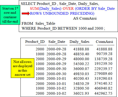
The first thing the above query does before calculating is SORT all the rows by Sale_Date. The Sort is located right after the ORDER BY.
CSUM – Rows Unbounded Preceding Explained
SELECT Product_ID , Sale_Date, Daily_Sales,
SUM(Daily_Sales) OVER (ORDER BY Sale_Date
ROWS UNBOUNDED PRECEDING) AS CsumAnsi
FROM Sales_Table
WHERE Product_ID BETWEEN 1000 and 2000 ;

The keywords Rows Unbounded Preceding determines that this is a CSUM. There are only a few different statements and Rows Unbounded Preceding is the main one. It means start calculating at the beginning row, and continue calculating until the last row.
CSUM – Making Sense of the Data
SELECT |
Product_ID , Sale_Date, Daily_Sales, |
|
SUM(Daily_Sales) OVER (ORDER BY Sale_Date |
|
ROWS UNBOUNDED PRECEDING) AS SUMOVER |
FROM Sales_Table WHERE Product_ID BETWEEN 1000 and 2000 ; |
|

The second “SUMOVER” row is 90739.28. That is derived by the first row’s Daily_Sales (41888.88) added to the SECOND row’s Daily_Sales (48850.40).
CSUM – Making Even More Sense of the Data
SELECT |
Product_ID , Sale_Date, Daily_Sales, |
|
SUM(Daily_Sales) OVER (ORDER BY Sale_Date |
|
ROWS UNBOUNDED PRECEDING) AS SUMOVER |
FROM Sales_Table WHERE Product_ID BETWEEN 1000 and 2000 ; |
|
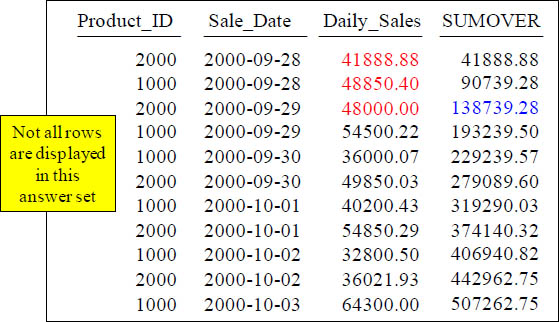
The third “SUMOVER” row is 138739.28. That is derived by taking the first row’s Daily_Sales (41888.88) and adding it to the SECOND row’s Daily_Sales (48850.40). Then, you add that total to the THIRD row’s Daily_Sales (48000.00).
CSUM – The Major and Minor Sort Key(s)
SELECT Product_ID , Sale_Date, Daily_Sales,
SUM(Daily_Sales) OVER (ORDER BY Product_ID, Sale_Date
ROWS UNBOUNDED PRECEDING) AS SumOVER
FROM Sales_Table ;

You can have more than one SORT KEY. In the top query, Product_ID is the MAJOR Sort, and Sale_Date is the MINOR Sort.
The ANSI CSUM – Getting a Sequential Number

With “Seq_Number”, because you placed the number 1 in the area which calculates the cumulative sum, it’ll continuously add 1 to the answer for each row.
Troubleshooting The ANSI OLAP on a GROUP BY
SELECT Product_ID , Sale_Date, Daily_Sales,
SUM(Daily_Sales) OVER (ORDER BY Sale_Date
ROWS UNBOUNDED PRECEDING) AS AnsiCsum
FROM Sales_Table
GROUP BY Product_ID ;
Error! Why?
Never GROUP BY in a SUM()Over or with any ANSI Syntax OLAP command. If you want to reset you use a PARTITION BY Statement, but never a GROUP BY.
Reset with a PARTITION BY Statement
SELECT Product_ID , Sale_Date, Daily_Sales,
SUM(Daily_Sales) OVER (PARTITION BY Product_ID
ORDER BY Product_ID, Sale_Date
ROWS UNBOUNDED PRECEDING) AS SumANSI
FROM Sales_Table ;

The PARTITION Statement is how you reset in ANSI. This will cause the SUMANSI to start over (reset) on its calculating for each NEW Product_ID.
PARTITION BY only Resets a Single OLAP not ALL of them
SELECT Product_ID , Sale_Date, Daily_Sales,
SUM(Daily_Sales) OVER (PARTITION BY Product_ID
ORDER BY Product_ID, Sale_Date
ROWS UNBOUNDED PRECEDING) AS Subtotal,
SUM(Daily_Sales) OVER (ORDER BY Product_ID, Sale_Date
ROWS UNBOUNDED PRECEDING) AS GrandTotal
FROM Sales_Table ;
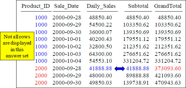
Above are two OLAP statements. Only one has PARTITION BY, so only it resets.
The Moving SUM (MSUM) and Moving Window
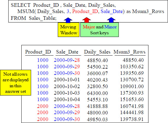
This is the Moving Sum (MSUM). It will calculate the Sum of 3 rows because that is the Moving Window. It will read the current row and TWO preceding to find the MSUM of those 3 rows. It will be sorted by Product_ID and Sale_Date first.
How the Moving Sum is Calculated
SELECT Product_ID , Sale_Date, Daily_Sales,
MSUM( Daily_Sales, 3, Product_ID, Sale_Date) as MSum3_Rows
FROM Sales_Table
With a Moving Window of 3, how is the 139350.69 amount derived in MSum3_Rows, which is in the third row? It is the SUM of 48850.40, 54500.22 and 36000.07. The fourth row has MSum3_Rows equal to 130700.72. That was the Sum of 54500.22, 360000.07 and 40200.43. The MSum is the current row sum plus the previous two.
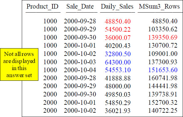
How the Sort works for Moving SUM (MSUM)
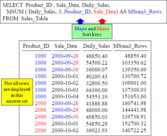
The sorting above is a major and minor sort. The major sort is on the product_id column and that sort is done first. For any duplicate product_id rows the minor sort takes effect. Notice that all of the product_id 1000's are further sorted by sale_date.
GROUP BY in the Moving SUM does a Reset
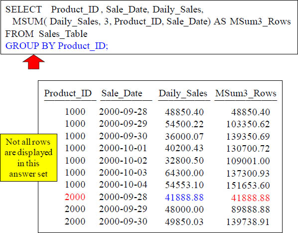
What does the GROUP BY Product_ID do? It causes a reset on all Product_ID breaks.
Quiz – Can you make the Advanced Calculation in your mind?

How is the 89888.88 derived in the 9th row of the MSum3_Rows?
Answer to Quiz for the Advanced Calculation in your mind?

The GROUP BY reset the column to start over when Product_ID went to 2000. The 89888.88 is the sum of 41888.88 and 48000.00.
Quiz – Write that Teradata Moving SUM in ANSI Syntax
SELECT Product_ID , Sale_Date, Daily_Sales,
MSUM( Daily_Sales, 3, Product_ID, Sale_Date) AS MSum3
FROM Sales_Table ;
Challenge
Can you place
another equivalent
Moving Sum
in the SQL above
using ANSI Syntax?
Here is a challenge that almost everyone fails. Can you do it perfectly?
Both the Teradata Moving SUM and ANSI Version
SELECT Product_ID , Sale_Date, Daily_Sales,
MSUM( Daily_Sales, 3, Product_ID, Sale_Date) AS MSum3,
SUM(Daily_Sales) OVER (ORDER BY Product_ID,
Sale_Date ROWS 2 Preceding) AS SUM3_ANSI
FROM Sales_Table ;
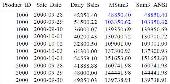
Not all rows are displayed in this answer set
The MSUM and SUM (Over) commands above are equivalent. Notice the Moving Window of 3 in the Teradata syntax is a 2 in the ANSI version. That is because in ANSI the moving window is considered the Current Row and 2 preceding.
ANSI Moving Window is Current Row and Preceding n Rows

The SUM () Over allows you to get the moving SUM of a certain column. The moving window in ANSI form always includes the current row. A Rows 2 Preceding statement means the current row and two preceding, which is a moving window of 3.
How ANSI Moving SUM Handles the Sort

The SUM OVER places the sort after the ORDER BY.
Quiz – How is that Total Calculated?
SELECT Product_ID , Sale_Date, Daily_Sales,
SUM(Daily_Sales) OVER (ORDER BY Product_ID, Sale_Date
ROWS 2 Preceding) AS Sum3_ANSI
FROM Sales_Table ;
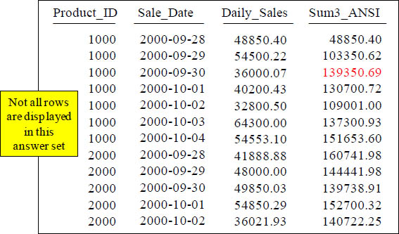
With a Moving Window of 3, how is the 139350.69 amount derived in the Sum3_ANSI column in the third row?
Answer to Quiz – How is that Total Calculated?
SELECT Product_ID , Sale_Date, Daily_Sales,
SUM(Daily_Sales) OVER (ORDER BY Product_ID, Sale_Date
ROWS 2 Preceding) AS Sum3_ANSI
FROM Sales_Table ;

With a Moving Window of 3, how is the 139350.69 amount derived in the Sum3_ANSI column in the third row? It is the sum of 48850.40, 54500.22 and 36000.07. The current row of Daily_Sales plus the previous two rows of Daily_Sales.
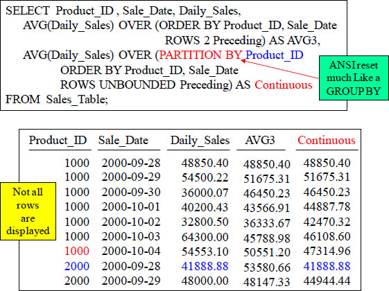
Moving SUM every 3-rows Vs a Continuous Average
SELECT Product_ID , Sale_Date, Daily_Sales,
SUM(Daily_Sales) OVER (ORDER BY Product_ID, Sale_Date
ROWS 2 Preceding) AS SUM3,
SUM(Daily_Sales) OVER (ORDER BY Product_ID, Sale_Date
ROWS UNBOUNDED Preceding) AS Continuous
FROM Sales_Table;

Not all rows are displayed in this answer set
The ROWS 2 Preceding gives the MSUM for every 3 rows. The ROWS UNBOUNDED Preceding gives the continuous MSUM.
Partition By Resets an ANSI OLAP

Use a PARTITION BY Statement to Reset the ANSI OLAP. Notice it only resets the OLAP command containing the Partition By statement, but not the other OLAPs.
The Moving Average (MAVG) and Moving Window

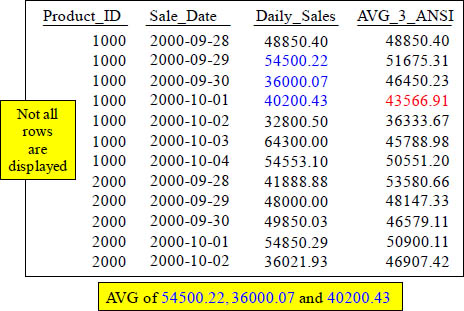
This is the Moving Average (MAVG). It will calculate the average of 3 rows because that is the Moving Window. It will read the current row and TWO preceding to find the MAVG of those 3 rows. It will be sorted by Product_ID and Sale_Date first.
How the Moving Average is Calculated
SELECT Product_ID , Sale_Date, Daily_Sales,
MAVG( Daily_Sales, 3, Product_ID, Sale_Date) AS AVG3_Rows
FROM Sales_Table ;
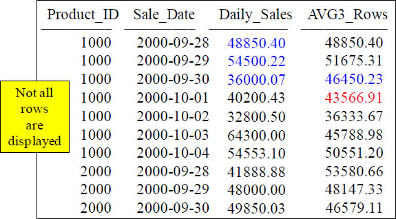
With a Moving Window of 3, how is the 46450.23 amount derived in the AVG3_Rows column in the third row? It is the AVG of 48850.40, 54500.22 and 36000.07! The fourth row has AVG3_Rows equal to 43566.91. That was the average of 54500.22, 360000.07 and 40200.43. The calculation is on the current row and the two before.
How the Sort works for Moving Average (MAVG)
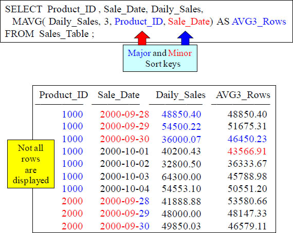
The sorting is show above.
GROUP BY in the Moving Average does a Reset
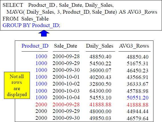
What does the GROUP BY Product_ID do? It causes a reset on all Product_ID breaks.
Quiz – Can you make the Advanced Calculation in your mind?
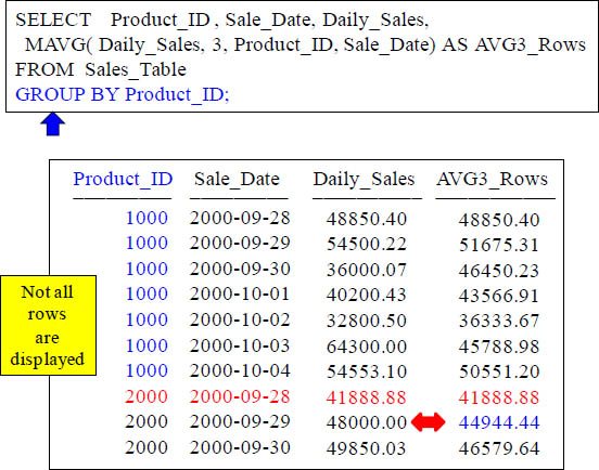
How is the 44944.44 derived in the 9th row of the AVG_for_3_Rows?.
Answer to Quiz for the Advanced Calculation in your mind?
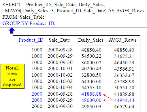
AVG of 41888.88 and 48000.00
Notice there are only two calculations although this has a moving window of 3. That is because the GROUP BY caused the MAVG to reset when Product_ID 2000 came.
Quiz – Write that Teradata Moving Average in ANSI Syntax
SELECT Product_ID , Sale_Date, Daily_Sales,
MAVG( Daily_Sales, 3, Product_ID, Sale_Date) AS AVG3_Rows
FROM Sales_Table ;
Challenge
Can you place
another equivalent
Moving Average
in the SQL above
using ANSI Syntax?
Here is a challenge that almost everyone fails. Can you do it perfectly?
Both the Teradata Moving Average and ANSI Version
SELECT Product_ID , Sale_Date, Daily_Sales,
MAVG( Daily_Sales, 3, Product_ID, Sale_Date) AS AVG_3,
AVG(Daily_Sales) OVER (ORDER BY Product_ID,
Sale_Date ROWS 2 Preceding) AS AVG_3_ANSI
FROM Sales_Table ;

The MAVG and AVG(Over) commands above are equivalent. Notice the Moving Window of 3 in the Teradata syntax and that it is a 2 in the ANSI version. That is because in ANSI it is considered the Current Row and 2 preceding.
Moving Average
SELECT Product_ID , Sale_Date, Daily_Sales,
AVG(Daily_Sales) OVER (ORDER BY Product_ID, Sale_Date
ROWS 2 Preceding) AS AVG_3
FROM Sales_Table ;

Notice the Moving Window of 3 in the syntax and that it is a 2 in the ANSI version. That is because in ANSI, it is considered the Current Row and 2 preceding.
The Moving Window is Current Row and Preceding
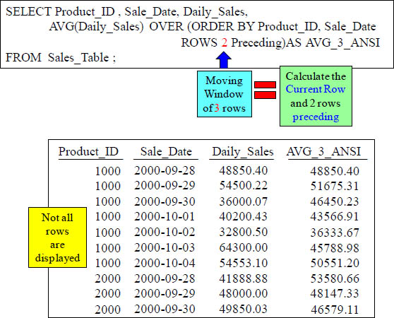
The AVG () Over allows you to get the moving average of a certain column. The Rows 2 Preceding is a moving window of 3 in ANSI.
How Moving Average Handles the Sort

Much like the SUM OVER Command, the Average OVER places the sort keys via the ORDER BY keywords.
Quiz – How is that Total Calculated?
SELECT Product_ID , Sale_Date, Daily_Sales,
AVG(Daily_Sales) OVER (ORDER BY Product_ID, Sale_Date
ROWS 2 Preceding) AS AVG_3_ANSI
FROM Sales_Table ;
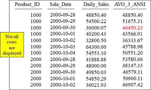
With a Moving Window of 3, how is the 46450.23 amount derived in the AVG_3_ANSI column in the third row?
Answer to Quiz – How is that Total Calculated?
SELECT Product_ID , Sale_Date, Daily_Sales,
AVG(Daily_Sales) OVER (ORDER BY Product_ID, Sale_Date
ROWS 2 Preceding) AS AVG_3_ANSI
FROM Sales_Table ;
AVG of 48850.40, 54500.22, and 36000.07
With a Moving Window of 3, the 46450.23 amount derived in the third row is the average of 48850.40, 54500.22, and 36000.07.
Quiz – How is that 4th Row Calculated?
SELECT Product_ID , Sale_Date, Daily_Sales,
AVG(Daily_Sales) OVER (ORDER BY Product_ID, Sale_Date
ROWS 2 Preceding) AS AVG_3_ANSI
FROM Sales_Table ;

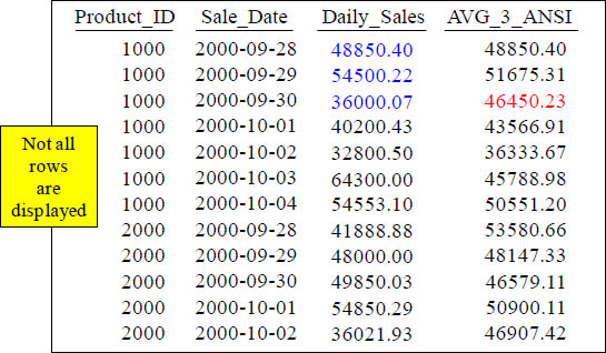
With a Moving Window of 3, how is the 43566.91 amount derived in the AVG_3_ANSI column in the fourth row?.
Answer to Quiz – How is that 4th Row Calculated?
SELECT Product_ID , Sale_Date, Daily_Sales,
AVG(Daily_Sales) OVER (ORDER BY Product_ID, Sale_Date
ROWS 2 Preceding) AS AVG_3_ANSI
FROM Sales_Table ;
With a Moving Window of 3, how is the 43566.91 amount derived in the AVG_3_ANSI column in the fourth row? The current row plus Rows 2 Preceding.
Moving Average every 3-rows Vs a Continuous Average
SELECT Product_ID , Sale_Date, Daily_Sales,
AVG(Daily_Sales) OVER (ORDER BY Product_ID, Sale_Date
ROWS 2 Preceding) AS AVG3,
AVG(Daily_Sales) OVER (ORDER BY Product_ID, Sale_Date
ROWS UNBOUNDED Preceding) AS Continuous
FROM Sales_Table;

The ROWS 2 Preceding gives the MAVG for every 3 rows. The ROWS UNBOUNDED Preceding gives the continuous MAVG.
Partition By Resets an ANSI OLAP
Use a PARTITION BY Statement to Reset the ANSI OLAP. The Partition By statement only resets the column using the statement. Notice that only Continuous resets.
The Moving Difference (MDIFF)

This is the Moving Difference (MDIFF). What this does is calculate the difference between the current row and only the 4th row preceding.
Moving Difference using ANSI Syntax
SELECT Product_ID, Sale_Date, Daily_Sales,
Daily_Sales - SUM(Daily_Sales)
OVER ( ORDER BY Product_ID ASC, Sale_Date ASC
ROWS BETWEEN 4 PRECEDING AND 4 PRECEDING)
AS "MDiff_ANSI"
FROM Sales_Table ;

This is how you do a MDiff using the ANSI Syntax with a moving window of 4.
Moving Difference using ANSI Syntax with Partition By
SELECT Product_ID, Sale_Date, Daily_Sales,
Daily_Sales - SUM(Daily_Sales) OVER (PARTITION BY Product_ID
ORDER BY Product_ID ASC, Sale_Date ASC
ROWS BETWEEN 4 PRECEDING AND 4 PRECEDING) AS "MDiff_ANSI"
FROM Sales_Table;

Wow! This is how you do a MDiff using the ANSI Syntax with a moving window of 4 and with a PARTITION BY statement.
Trouble Shooting the Moving Difference (MDIFF)
SELECT Product_ID , Sale_Date, Daily_Sales,
MDIFF(Daily_Sales, 7, Product_ID, Sale_Date) as Compare2Rows
FROM Sales_Table GROUP BY Product_ID ;

Do you notice that column Compare2Rows did not produce any data? That is because the GROUP BY Reset before it could get 7 records to find the MDIFF.
Using the RESET WHEN Option in Teradata V13
SELECT Product_ID, Sale_Date, Daily_Sales,
ROW_NUMBER() OVER (PARTITION BY Product_ID ORDER BY Sale_Date
RESET WHEN Daily_Sales <= SUM(Daily_Sales)
OVER (PARTITION BY Product_ID
ORDER BY Sale_Date
ROWS BETWEEN 1 PRECEDING AND 1 PRECEDING)) -1 as Increases
FROM Sales_Table WHERE Product_ID Between 1000 and 2000 ;

This query finds how many consecutive days the Daily_Sales increases per product_id.
How Many Months Per Product_ID Has Revenue Increased?
SELECT Product_ID, Month(Sale_Date) as Mo, sum(Daily_Sales)
as Monthly_Sum,
ROW_NUMBER() over (PARTITION BY Product_ID
ORDER BY Mo
RESET WHEN sum(Daily_Sales) <=SUM(sum(Daily_Sales))
over (PARTITION BY Product_ID
ORDER BY Mo
ROWS BETWEEN 1 PRECEDING AND 1 PRECEDING)) -1 as
Balance_Increase
FROM Sales_Table
GROUP BY Product_ID, Mo;

This query finds how many months per Product_ID the revenue has increased.
The RANK Command
SELECT Product_ID ,Sale_Date , Daily_Sales,
RANK(Daily_Sales) AS "Rank"
FROM Sales_Table WHERE Product_ID IN (1000, 2000) ;
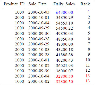
This is the RANK. In this example, it will rank your Daily_Sales from greatest to least. The default for this type of RANK is to sort DESC.
How to get Rank to Sort in Ascending Order
SELECT Product_ID ,Sale_Date , Daily_Sales,
RANK(Daily_Sales ASC) AS "Rank"
FROM Sales_Table WHERE Product_ID IN (1000, 2000) ;

This RANK query sorts in Ascending mode.
Two ways to get Rank to Sort in Ascending Order
SELECT Product_ID ,Sale_Date , Daily_Sales,
RANK(Daily_Sales ASC) AS Rank1,
RANK(-Daily_Sales) AS Rank2
FROM Sales_Table WHERE Product_ID IN (1000, 2000) ;
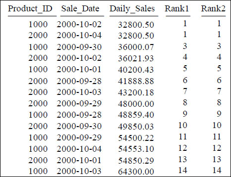
A minus sign or keyword ASC will sort RANK in Ascending mode.
RANK Defaults to Ascending Order
SELECT Product_ID ,Sale_Date , Daily_Sales,
RANK() OVER (ORDER BY Daily_Sales) AS Rank1
FROM Sales_Table
WHERE Product_ID IN (1000, 2000) ;

This is the RANK() OVER. It provides a rank for your queries. Notice how you do not place anything within the () after the word RANK. Default Sort is ASC.
Getting RANK to Sort in DESC Order
SELECT Product_ID ,Sale_Date , Daily_Sales,
RANK() OVER (ORDER BY Daily_Sales DESC)
AS Rank1
FROM Sales_Table WHERE Product_ID IN (1000, 2000) ;
Is the query above in ASC mode or DESC mode for sorting?
RANK() OVER and PARTITION BY
SELECT Product_ID ,Sale_Date , Daily_Sales,
RANK() OVER (PARTITION BY Product_ID
ORDER BY Daily_Sales DESC) AS Rank1
FROM Sales_Table WHERE Product_ID IN (1000, 2000) ;
What does the PARTITION Statement in the RANK() OVER do? It resets the rank.
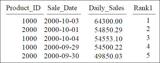
RANK() OVER And QUALIFY
SELECT Product_ID, Sale_Date, Daily_Sales,
RANK() OVER (ORDER BY Daily_Sales DESC) AS Rank1
FROM Sales_Table
WHERE Product_ID IN (1000, 2000)
QUALIFY Rank1 < 7
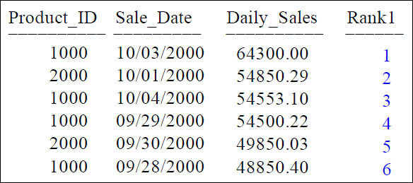
The QUALIFY statement limits rows once the Rank’s been calculated.
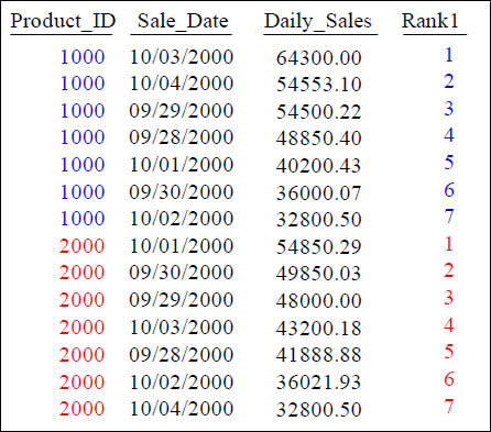
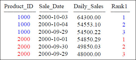
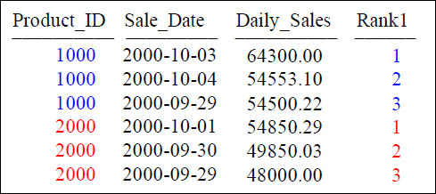
RANK() OVER and PARTITION BY with a QUALIFY
SELECT Product_ID ,Sale_Date , Daily_Sales,
RANK() OVER (PARTITION BY Product_ID
ORDER BY Daily_Sales DESC) AS Rank1
FROM Sales_Table
WHERE Product_ID IN (1000, 2000)
QUALIFY Rank1 < 4

What does the PARTITION Statement in the RANK() OVER do? It resets the rank. The QUALIFY statement limits rows once the Rank’s been calculated.
QUALIFY and WHERE
SELECT Product_ID ,Sale_Date , Daily_Sales,
RANK(Daily_Sales ASC) AS Rank1,
RANK(-Daily_Sales) AS Rank2
FROM Sales_Table
WHERE Product_ID IN (1000, 2000)
QUALIFY Rank(-Daily_Sales) < 6 ;

The WHERE statement is performed first. It limits the rows being calculated. Then the QUALIFY takes the calculated rows and limits the returning rows. QUALIFY is to OLAP what HAVING is to Aggregates. Both limit after the calculations. Notice that our Rank1 and Rank2 are exactly the same because we sorted them both the same.
Quiz – How can you simplify the QUALIFY Statement?
SELECT Product_ID ,Sale_Date , Daily_Sales,
RANK(Daily_Sales ASC) AS Rank1,
RANK(-Daily_Sales) AS Rank2
FROM Sales_Table
WHERE Product_ID IN (1000, 2000)
QUALIFY Rank(-Daily_Sales) < 6 ;

How can you improve the QUALIFY Statement above for simplicity?
Answer to Quiz –Can you simplify the QUALIFY Statement
SELECT Product_ID ,Sale_Date , Daily_Sales,
RANK(Daily_Sales ASC) AS Rank1,
RANK(-Daily_Sales) AS Rank2
FROM Sales_Table
WHERE Product_ID IN (1000, 2000)
QUALIFY Rank2 < 6 ;

QUALIFY Rank2 < 6 (Use the Alias)
The QUALIFY Statement without Ties
SELECT Product_ID ,Sale_Date , Daily_Sales,
RANK(Daily_Sales) AS Rank1
FROM Sales_Table
WHERE Product_ID IN (1000, 2000)
QUALIFY Rank1 < 6 ;
A QUALIFY < 6 will provide a result that is 5 rows. Notice there are NO ties, yet! This is merely because we have no ties, but turn to the next page and we will have.
The QUALIFY Statement with Ties
SELECT Product_ID ,Sale_Date , Daily_Sales,
RANK(Daily_Sales ASC) AS Rank1
FROM Sales_Table
WHERE Product_ID IN (1000, 2000)
QUALIFY Rank1 < 6 ;
A QUALIFY < 6 will provide a result that is five rows. Notice there are Ties! This is because in ASC mode there are two matches within our first five rows.
The QUALIFY Statement with Ties Brings back Extra Rows
SELECT Product_ID ,Sale_Date , Daily_Sales,
RANK(Daily_Sales ASC) AS Rank1
FROM Sales_Table
WHERE Product_ID IN (1000, 2000)
QUALIFY Rank1 < 2 ;

A QUALIFY < 2 will provide more rows than 1 because of the Ties!
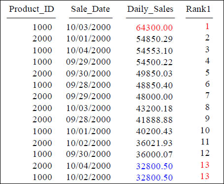
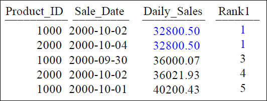
Mixing Sort Order for QUALIFY Statement
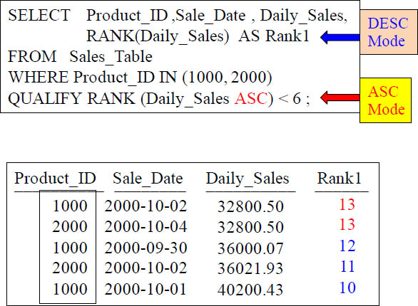
Look at the Rankings and the Daily_Sales. This data come out odd because Rank1 is DESC by default (using this Syntax) and the QUALIFY specifies ASC mode.
Quiz – What Caused the RANK to Reset?
SELECT Product_ID ,Sale_Date , Daily_Sales,
RANK(Daily_Sales) AS Rank1
FROM Sales_Table
WHERE Product_ID IN (1000, 2000)
GROUP BY Product_ID
QUALIFY Rank1 < 4 ;
What caused the data to reset the column Rank1?
Answer to Quiz – What Caused the RANK to Reset?
SELECT Product_ID ,Sale_Date , Daily_Sales,
RANK(Daily_Sales) AS Rank1
FROM Sales_Table
WHERE Product_ID IN (1000, 2000)
GROUP BY Product_ID
QUALIFY Rank1 < 4 ;
GROUP BY
What caused the data to reset the column Rank1? It is the GROUP BY statement.
Quiz – Name those Sort Orders
RANK() OVER (ORDER BY Daily_Sales) AS ANSI_Rank
Is the default above ASC or DESC?
RANK(Daily_Sales) AS NON_ANSI_Rank
Is the default above ASC or DESC?
Answer the questions above.
Answer to Quiz – Name those Sort Orders
RANK() OVER (ORDER BY Daily_Sales) AS ANSI_Rank
Defaults to ASC
RANK(Daily_Sales) AS NON_ANSI_Rank
Defaults to DESC
Please note that by default these different syntaxes sort completely opposite.
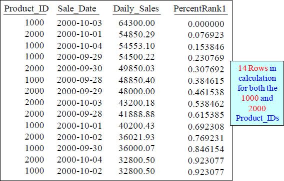
PERCENT_RANK() OVER
SELECT Product_ID ,Sale_Date , Daily_Sales,
PERCENT_RANK() OVER (PARTITION BY PRODUCT_ID
ORDER BY Daily_Sales DESC) AS PercentRank1
FROM Sales_Table WHERE Product_ID in (1000, 2000) ;

We now have added a Partition statement which resets on Product_ID so this produces 7 rows for each of our Product_IDs.
PERCENT_RANK() OVER with 14 rows in Calculation
SELECT Product_ID ,Sale_Date , Daily_Sales,
PERCENT_RANK()
OVER ( ORDER BY Daily_Sales DESC) AS PercentRank1
FROM Sales_Table WHERE Product_ID IN (1000, 2000) ;
Percentage_Rank is just like RANK however, it gives you the Rank as a percent, but only a percent of all the other rows up to 100%.
PERCENT_RANK() OVER with 21 rows in Calculation
SELECT Product_ID ,Sale_Date , Daily_Sales,
PERCENT_RANK() OVER ( ORDER BY Daily_Sales DESC)
AS PercentRank1
FROM Sales_Table ;
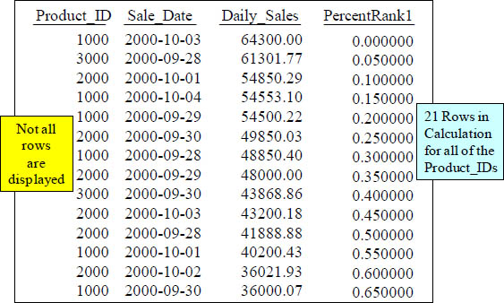
Percentage_Rank is just like RANK, however, it gives you the Rank as a percent but only a percent of all the other rows up to 100%.
Quiz – What Causes the Product_ID to Reset?
SELECT Product_ID ,Sale_Date , Daily_Sales,
PERCENT_RANK() OVER (PARTITION BY PRODUCT_ID
ORDER BY Daily_Sales DESC) AS PercentRank1
FROM Sales_Table WHERE Product_ID in (1000, 2000) ;

What caused the Product_IDs to be sorted?
Answer to Quiz – What Cause the Product_ID to Reset?
SELECT Product_ID ,Sale_Date , Daily_Sales,
PERCENT_RANK() OVER (PARTITION BY PRODUCT_ID
ORDER BY Daily_Sales DESC) AS PercentRank1
FROM Sales_Table WHERE Product_ID in (1000, 2000) ;

What caused the Product_IDs to be sorted? It was the PARTITION BY statement.
COUNT OVER for a Sequential Number
SELECT Product_ID ,Sale_Date , Daily_Sales,
COUNT(*) OVER (ORDER BY Product_ID, Sale_Date
ROWS UNBOUNDED PRECEDING) AS Seq_Number
FROM Sales_Table WHERE Product_ID IN (1000, 2000) ;
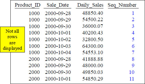
This is the COUNT OVER. It will provide a sequential number starting at 1. The Keyword(s) ROWS UNBOUNDED PRECEDING causes Seq_Number to start at the beginning and increase sequentially to the end.
Troubleshooting COUNT OVER
SELECT Product_ID ,Sale_Date , Daily_Sales,
COUNT(*) OVER (ORDER BY Product_ID, Sale_Date) AS No_Seq
FROM Sales_Table WHERE Product_ID IN (1000, 2000) ;
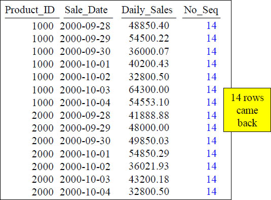
When you don’t have a ROWS UNBOUNDED PRECEDING, No_Seq gets a value of 14 on every row. Why? Because 14 is the FINAL COUNT NUMBER.
Quiz – What caused the COUNT OVER to Reset?
SELECT Product_ID ,Sale_Date , Daily_Sales,
COUNT(*) OVER (PARTITION BY Product_ID
ORDER BY Product_ID, Sale_Date
ROWS UNBOUNDED PRECEDING) AS StartOver
FROM Sales_Table WHERE Product_ID IN (1000, 2000) ;
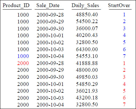
What Keyword(s) caused StartOver to reset?
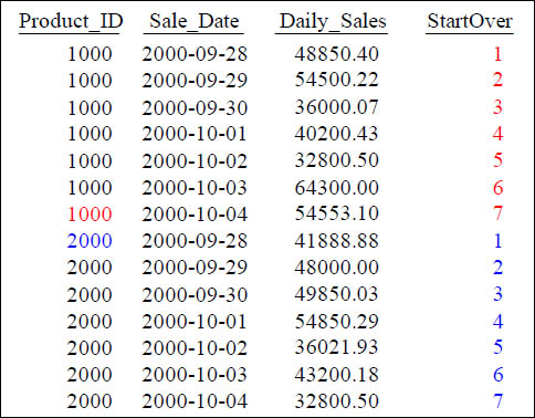
Answer to Quiz – What caused the COUNT OVER to Reset?
SELECT Product_ID ,Sale_Date , Daily_Sales,
COUNT(*) OVER (PARTITION BY Product_ID
ORDER BY Product_ID, Sale_Date
ROWS UNBOUNDED PRECEDING) AS StartOver
FROM Sales_Table WHERE Product_ID IN (1000, 2000) ;

What Keyword(s) caused StartOver to reset? It is the PARTITION BY statement.
The MAX OVER Command
SELECT Product_ID ,Sale_Date , Daily_Sales,
MAX(Daily_Sales) OVER (ORDER BY Product_ID, Sale_Date
ROWS UNBOUNDED PRECEDING) AS MaxOver
FROM Sales_Table WHERE Product_ID IN (1000, 2000) ;
After the sort, the Max() Over shows the Max Value up to that point.
MAX OVER with PARTITION BY Reset
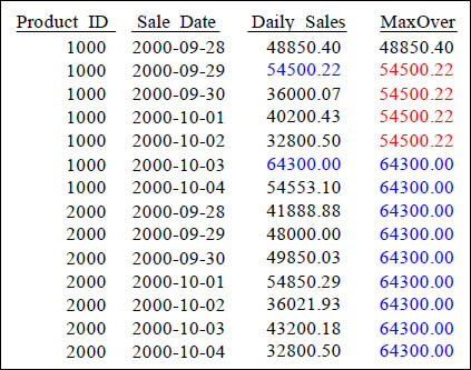
SELECT Product_ID ,Sale_Date , Daily_Sales,
MAX(Daily_Sales) OVER (PARTITION BY Product_ID
ORDER BY Product_ID, Sale_Date
ROWS UNBOUNDED PRECEDING) AS MaxOver
FROM Sales_Table WHERE Product_ID IN (1000, 2000) ;

The largest value is 64300.00 in the column MaxOver. Once it was evaluated, it did not continue until the end because of the PARTITION BY reset.
Troubleshooting MAX OVER
SELECT Product_ID ,Sale_Date , Daily_Sales,
MAX(Daily_Sales) OVER (ORDER BY Product_ID, Sale_Date )
AS MaxOver
FROM Sales_Table WHERE Product_ID IN (1000, 2000) ;

You can also use MAX as a OLAP. 64300.00 came back in MaxOver because that was the MAX value for Daily_Sales in this Answer Set. Notice that it doesn’t have a ROWS UNBOUNDED PRECEDING.
The MIN OVER Command
SELECT Product_ID, Sale_Date ,Daily_Sales
,MIN(Daily_Sales) OVER (ORDER BY Product_ID, Sale_Date
ROWS UNBOUNDED PRECEDING) AS MinOver
FROM Sales_Table WHERE Product_ID IN (1000, 2000) ;

After the sort, the MIN () Over shows the Max Value up to that point.
Troubleshooting MIN OVER
SELECT Product_ID ,Sale_Date , Daily_Sales,
MIN(Daily_Sales) OVER (ORDER BY Product_ID, Sale_Date )
AS MinOver
FROM Sales_Table WHERE Product_ID IN (1000, 2000) ;
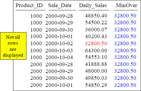
Min only displayed 32800.50 because there is NOT a ROWS UNBOUNDED PRECEDING statement so it found the lowest Daily_Sales and repeated it.
Finding a Value of a Column in the Next Row with MIN
SELECT Product_ID, Sale_Date, Daily_Sales,
MIN(Daily_Sales) OVER (PARTITION BY Product_ID
ORDER BY Product_ID, Sale_Date
ROWS BETWEEN 1 Following and 1 Following) AS NextSale
FROM Sales_Table WHERE Product_ID IN (1000, 2000) ;

The above example finds the value of a column in the next row for Daily_Sales. Notice it is partitioned, so there is a Null value at the end of each Product_ID.
Finding Gaps Between Dates
SELECT Product_Id, Sale_Date,
MIN(Sale_Date) OVER (PARTITION BY Product_Id
ORDER BY Sale_Date
ROWS BETWEEN 1 FOLLOWING
AND UNBOUNDED FOLLOWING) AS Date_Of_Next_Row
,Date_Of_Next_Row -Sale_Date AS Days_To_Next_Row
FROM Sales_Table WHERE Product_ID Between 1000 and 2000 ;

The above query finds gaps in dates.
The CSUM For Each Product_Id For The First 3 Days

The above example shows the cumulative SUM for the Daily_Sales for the first three days for each of our Product_IDs.
Quiz – Fill in the Blank
SELECT Product_ID ,Sale_Date , Daily_Sales,
MIN(Daily_Sales) OVER (PARTITION BY Product_ID
ORDER BY Product_ID, Sale_Date
ROWS UNBOUNDED PRECEDING) AS MinOver
FROM Sales_Table WHERE Product_ID IN (1000, 2000) ;
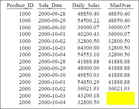
The last two answers (MinOver) are blank, so you can fill in the blank.
Answer – Fill in the Blank
SELECT Product_ID ,Sale_Date , Daily_Sales,
MIN(Daily_Sales) OVER (PARTITION BY Product_ID
ORDER BY Product_ID, Sale_Date
ROWS UNBOUNDED PRECEDING) AS MinOver
FROM Sales_Table WHERE Product_ID IN (1000, 2000) ;

The last two answers (MinOver) are filled in.
The Row_Number Command
SELECT Product_ID ,Sale_Date , Daily_Sales,
ROW_NUMBER() OVER
(ORDER BY Product_ID, Sale_Date) AS Seq_Number
FROM Sales_Table WHERE Product_ID IN (1000, 2000) ;
The ROW_NUMBER() Keyword(s) caused Seq_Number to increase sequentially. Notice that this does NOT have a Rows Unbounded Preceding, and it still works!
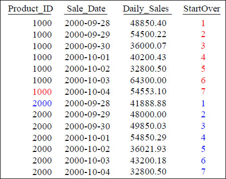
Quiz – How did the Row_Number Reset?
SELECT Product_ID ,Sale_Date , Daily_Sales,
ROW_NUMBER() OVER (PARTITION BY Product_ID
ORDER BY Product_ID, Sale_Date ) AS StartOver
FROM Sales_Table WHERE Product_ID IN (1000, 2000) ;
What Keyword(s) caused StartOver to reset?
Quiz – How did the Row_Number Reset?
SELECT Product_ID ,Sale_Date , Daily_Sales,
ROW_NUMBER() OVER (PARTITION BY Product_ID
ORDER BY Product_ID, Sale_Date ) AS StartOver
FROM Sales_Table WHERE Product_ID IN (1000, 2000) ;
What Keyword(s) caused StartOver to reset? It is the PARTITION BY statement.
Row_Number With Qualify to get the Typical Rows Per Value
SELECT Counter AS "Typical Rows per Value"
FROM
(SELECT Product_ID, COUNT(*)
FROM Sales_Table GROUP BY 1) AS TeraTom (Col1, Counter),
(SELECT COUNT(DISTINCT(Product_ID))
FROM Sales_Table) AS Derived2 (num_rows)
QUALIFY ROW_NUMBER () OVER
(ORDER BY TeraTom.Col1) = Derived2.num_rows /2 ;
Typical Rows Per Value
7
The query above retrieved the typical rows per value for the column Product_ID.
A Second Typical Rows Per Value Query on Sale_Date
SELECT Counter AS "Typical Rows per Sale_Date"
FROM
(SELECT Sale_Date, COUNT(*)
FROM Sales_Table GROUP BY 1) AS TeraTom (Col1, Counter),
(SELECT COUNT(DISTINCT(Sale_Date))
FROM Sales_Table) AS Derived2 (num_rows)
QUALIFY ROW_NUMBER () OVER
(ORDER BY TeraTom.Col1) = Derived2.num_rows /2 ;
Typical Rows Per Sale_Date
3
The query above retrieved the typical rows per value for the column Sale_Date.