Chapter 17 - Table Create and Data Types
“I Create a definite plan for carrying out your desire and begin at once, whether you are ready or not, to put this plan into action.”
– Napoleon Hill
Creating a Table With A Unique Primary Index (UPI)
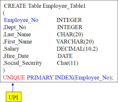
This is a basic TABLE CREATE STATEMENT. You have Columns and the data types in them. As you see, the Primary Index is defined for a Table at TABLE CREATE time.
Creating a Table With A Non-Unique Primary Index (NUPI)
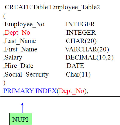
A Non-Unique Primary Index (NUPI) is on the above table. Notice how you only need to put ‘Primary Index’.
Creating a Table With A Multi-Column Primary Index
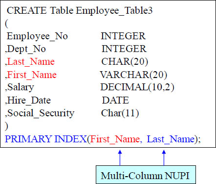
A Non-Unique Primary Index (NUPI) is on the above table. It has only one primary index, but this primary index is made up of the combination of both First_Name and Last_Name columns. This is often done because it provides better distribution or both columns are often used together to query the table. Both columns are needed in the WHERE and the additional AND clause for the system to be able to utilize a single-AMP retrieve.
Creating a Table With No Primary Index

The above example represents a No Primary Index table. This is referred to a NoPI because it has no primary index. This will automatically spread the data evenly in a round robin fashion. It is often used in a staging table scenario for the ETL process (Extract, Transform and Load). A NoPI table is also a requirement for a table if it is a Columnar Table.
Creating a Table Without Entering a Primary Index Definition

Here we have created a table without defining the Primary Index. This will either default to making a Non-Unique Primary Index of the first or make it a No Primary Index table. It depends on the system setting in DBS Control.
Creating a SET Table
CREATE SET Table Employee_Table6
(
Employee_No |
INTEGER |
,Dept_No |
INTEGER |
,Last_Name |
CHAR(20) |
,First_Name |
VARCHAR(20) |
,Salary |
DECIMAL(10,2) |
,Hire_Date |
DATE |
,Social_Security |
Char(11) |
)
PRIMARY INDEX(Dept_No);
A SET table does not allow a duplicate row in the table. The system has to do a Duplicate Row Check for data loads, which slows down the data loading process, but if someone loads the data twice the duplicate rows are automatically rejected and kicked out.
SET TABLE means that Duplicate ROWS are rejected. If your system is in Teradata mode then SET tables will be the default.
Creating a MULTISET Table
CREATE MULTISET Table Employee_Table7
(
Employee_No |
INTEGER |
,Dept_No |
INTEGER |
,Last_Name |
CHAR(20) |
,First_Name |
VARCHAR(20) |
,Salary |
DECIMAL(10,2) |
,Hire_Date |
DATE |
,Social_Security |
Char(11) |
)
PRIMARY INDEX(Employee_No);
A MULTISET table does allow duplicate rows in the table. The system does not have to do a Duplicate Row Check for data loads. If someone accidentally loads the data twice the duplicate rows are placed inside the table.
A MULTISET Table means the table will ALLOW duplicate rows. If your system is in ANSI mode then MULTISET tables will be the default. In either Teradata mode or ANSI mode you can specifically state (SET or MULTISET) for the table type desired.
Creating a SET Table With a Unique Primary Index
CREATE SET Table Employee_Table8
(
Employee_No |
INTEGER |
,Dept_No |
INTEGER |
,Last_Name |
CHAR(20) |
,First_Name |
VARCHAR(20) |
,Salary |
DECIMAL(10,2) |
,Hire_Date |
DATE |
,Social_Security |
Char(11) |
)
UNIQUE PRIMARY INDEX(Employee_No)
UNIQUE INDEX (Social_Security) ;
A SET table never does a "duplicate row check" if there is a UNIQUE constraint on the table. That constraint comes from either having a Unique Primary Index (UPI) or a Unique Secondary Index (USI). The above example has both.
It is very important when dealing with a SET table to have either a Unique Primary Index or a Unique Secondary Index. They eliminate the Duplicate Row Check. Because SET tables won’t allow duplicate rows a “Duplicate Row Check” is done on all new INSERTS or UPDATES, but if any column has a UNIQUE constraint then the system knows that no row can be duplicate because the specific column is UNIQUE. This saves a lot of time with loads and maintenance. Do your best to stay away from the Duplicate Row Check when you can.
Creating a Table With Multiple Secondary Indexes
CREATE Table Employee_Table9
(
Employee_No |
INTEGER |
,Dept_No |
INTEGER |
,Last_Name |
CHAR(20) |
,First_Name |
VARCHAR(20) |
,Salary |
DECIMAL(10,2) |
,Hire_Date |
DATE |
,Social_Security |
Char(11) |
) Unique Primary Index (Employee_No)
Unique Index (Social_Security)
Index(Dept_No) ;
This table has an UPI, USI and NUSI
Above we have three indexes on the table. We have a Unique Primary Index on Employee_No. We have a Unique Secondary Index on Social_Security and we have a Non-Unique Secondary Index on Dept_No.
Creating a PPI Table with Simple Partitioning
CREATE Table Employee_Table_PPI
(
Employee_No |
INTEGER |
,Dept_No |
INTEGER |
,Last_Name |
CHAR(20) |
,First_Name |
VARCHAR(20) |
,Salary |
DECIMAL(10,2) |
) Primary Index (Employee_No)
PARTITION BY (Dept_No) ;
Data is still spread across the AMPs by hashing of the Primary Index of Employee_No, but AMPs will sort the rows they receive by Dept_No.
Each AMP can have 65,535 partitions per table, but after Teradata V14 each AMP can have 9.223 Quintillion partitions per table.
Above we have an example of a PPI table. PPI stands for Partitioned Primary Index. A PPI table only indicates how an AMP should sort the rows distributed to them. In this case the AMPs will sort by Dept_No. This is a form of Simple Partitioning.
Creating a PPI Table with RANGE_N Partitioning per Month
CREATE TABLE Order_Table_PPI1
(Order_Number |
INTEGER Not Null |
,Customer_Number |
INTEGER |
,Order_Date |
DATE |
,Order_Total |
Decimal (10,2) |
) PRIMARY INDEX(Order_Number)
PARTITION BY RANGE_N (Order_Date
BETWEEN date '2012-01-01'
AND date '2012-06-30'
EACH INTERVAL '1' Month);
Above we have an example of a Partitioned Primary Index (PPI) table. This is a RANGE_N partition. The AMPs will distribute the data by Order_Number because it is the Primary Index, but each AMP will sort the rows it is assigned by month of Order_Date. This is done for range queries so they won’t have to perform a full table scan, but instead can have all of the AMPs read only certain partitions in order to satisfy the query.
Creating a PPI Table with RANGE_N Partitioning per Day
CREATE TABLE Order_Table_PPI2
(Order_Number |
INTEGER Not Null |
,Customer_Number |
INTEGER |
,Order_Date |
DATE |
,Order_Total |
Decimal (10,2) |
) PRIMARY INDEX(Order_Number)
PARTITION BY RANGE_N (Order_Date
BETWEEN date '2012-01-01'
AND date '2012-12-31'
EACH INTERVAL '1' Day);

Above we have an example of a Partitioned Primary Index (PPI) table. This is a RANGE_N partition. The AMPs will distribute the data by Order_Number because it is the Primary Index, but each AMP will sort the rows it is assigned by day of Order_Date. This is done for range queries so they won’t have to perform a full table scan, but instead can have all of the AMPs read only certain partitions in order to satisfy the query.
Creating a PPI Table with RANGE_N Partitioning per Week
CREATE TABLE Order_Table_PPI2
(Order_Number |
INTEGER Not Null |
,Customer_Number |
INTEGER |
,Order_Date |
DATE |
,Order_Total |
Decimal (10,2) |
) PRIMARY INDEX(Order_Number)
PARTITION BY RANGE_N (Order_Date
BETWEEN date '2012-01-01'
AND date '2012-12-31'
EACH INTERVAL '1' Week);
Above we have an example of a Partitioned Primary Index (PPI) table. This is a RANGE_N partition. The AMPs will distribute the data by Order_Number because it is the Primary Index, but each AMP will sort the rows it is assigned by Order_Date (each week is one partition). This is done for range queries so they won’t have to perform a full table scan, but instead can have all of the AMPs read only certain partitions in order to satisfy the query.
A Clever Range_N Option
CREATE MULTISET TABLE Telco_Routing
(
Year_ID INTEGER,
Month_ID INTEGER,
Subscriber_ID INTEGER,
Connect_Date VARCHAR(40),
Disconnect_Date VARCHAR(40),
Revenue_1_MTH DECIMAL(18,2),
Revenue_2_MTH DECIMAL(18,2),
Revenue_3_MTH DECIMAL(18,2),
Average_Revenue DECIMAL(18,2))
PRIMARY INDEX ( Subscriber_ID )
Partition by Range_N(Subscriber_ID
BETWEEN 1 and 500000000 each 10000);
Above we have an example of a Partitioned Primary Index (PPI) table. This is a RANGE_N partition. The AMPs will distribute the data by Subscriber_ID because it is the Primary Index, but each AMP will sort the rows it is assigned by Subscriber_ID (not the row-id after Subscriber_ID is hashed). This is done for range queries so they won’t have to perform a full table scan, but instead can have all of the AMPs read only certain partitions in order to satisfy the query. There will be 10000 Subscriber_IDs per partition.
Creating a PPI Table with CASE_N
CREATE TABLE Order_Table_CPPI
(Order_Number |
INTEGER Not Null |
,Customer_Number |
INTEGER |
,Order_Date |
DATE |
,Order_Total |
Decimal (10,2) |
)
PRIMARY INDEX(Order_Number)
PARTITION BY CASE_N
(Order_Total < 1000,
Order_Total < 5000,
Order_Total < 10000,
Order_Total < 20000,
NO Case, UNKNOWN);
Above we have an example of a Partitioned Primary Index (PPI) table. This is a CASE_N partition. The AMPs will distribute the data by Order_Number because it is the Primary Index, but each AMP will sort the rows it is assigned by the CASE statement. This is done for range queries so they won’t have to perform a full table scan, but instead can have all of the AMPs read only certain partitions in order to satisfy the query. There will be six partitions here. One partition for orders < 1000, another for orders between 1000 and 5000 (not inclusive) and so on. There will also be a partition when an Order_Total is > 20000 (No Case) and for rows where the Order_Total is null (UNKNOWN).
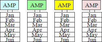
The No Case and Unknown Partition Options
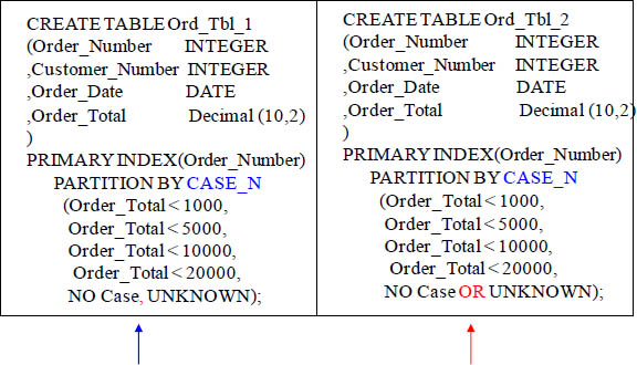
Notice both examples and the No CASE and UNKNOWN partitions. The first example (on the left) has a separate partition for the No Case and the UNKNOWN partitions, but the second example combines these two partitions together.
Partitioning of Older and Newer Data Separately
CREATE TABLE Order_Table_MultiYear
(Order_Number |
INTEGER Not Null |
,Customer_Number |
INTEGER |
,Order_Date |
DATE |
,Order_Total |
Decimal (10,2) |
)
PRIMARY INDEX(Order_Number)
PARTITION BY RANGE_N
(Order_Date BETWEEN
Date '2005-01-01' AND date '2009-12-31'
EACH INTERVAL '1' MONTH,
Date '2010-01-01' AND date '2010-12-31'
EACH INTERVAL '1' DAY );
The above example will take older data and partition it by month and partition the newer data by day.
Multi-Level Partitioning
CREATE TABLE Order_TableMLPPI
(Order_Number |
INTEGER Not Null |
,Customer_Number |
INTEGER |
,Order_Date |
DATE |
,Order_Total |
Decimal (10,2) |
) PRIMARY INDEX(Order_Number)
PARTITION BY (RANGE_N (Order_Date BETWEEN
Date '2012-01-01' AND date '2012-12-31'
EACH INTERVAL '1' DAY) ,
CASE_N (Order_Total < 1000,
Order_Total < 5000,
Order_Total < 10000,
Order_Total < 20000,
No Case));
The above example is a form of Multi-Level partitioning. The data will first be sorted on each AMP by a RANGE_N and then further sorted the CASE_N statement. This delivers a finer level of granularity so even less partitions might potentially be read to satisfy a query. There are three partitioning standards and they are Simple, Range_N, and Case_N. Multi-Level partitioning (up to 15 levels) can only be a combination of RANGE_N and CASE_N combinations.
Almost All PPI Tables have a Non-Unique Primary Index
CREATE Set TABLE Order_Table_Non
(Order_Number |
INTEGER Not Null |
,Customer_Number |
INTEGER |
,Order_Date |
DATE |
,Order_Total |
Decimal (10,2) |
) PRIMARY INDEX(Order_Number)
PARTITION BY CASE_N
(Order_Total < 1000,
Order_Total < 5000,
Order_Total < 10000,
Order_Total < 20000,
NO Case OR UNKNOWN);
A PPI table cannot have a Unique Primary Index (UPI) unless the Primary Index is included as part of the partitioning statement. Since it is not (in this example) the table cannot have a Unique Primary Index.
All PPI tables have to have a Non-Unique Primary Index unless the partition statement includes the Primary Index column. Above, we have a Primary Index on Order_Number, but the partition is a CASE_N on Order_Total. Teradata will error if you try and put a Unique Primary Index statement in.
PPI Table With a Unique Primary Index (UPI)
CREATE TABLE Order_Table_UPI
(Order_Number |
INTEGER Not Null |
,Customer_Number |
INTEGER |
,Order_Date |
DATE |
,Order_Total |
Decimal (10,2) |
) UNIQUE PRIMARY INDEX(Order_Number, Order_Total)
PARTITION BY CASE_N
( Order_Total < 1000,
Order_Total < 5000,
Order_Total < 10000,
Order_Total < 20000,
NO Case OR UNKNOWN);
A PPI table cannot have a Unique Primary Index (UPI) unless the Primary Index is included as part of the partitioning statement. Since it is (in this example) the table can have a Unique Primary Index.
All PPI tables have to have a Non-Unique Primary Index unless the partition statement includes the Primary Index column. Above, we have a multi-column Primary Index on both Order_Number and Order_Total. Since the partition is on Order_Total Teradata will allow a Unique Primary Index.
Clever Trick for PPI Tables
CREATE TABLE Order_Table_Tricks
(Order_Number |
INTEGER Not Null |
,Customer_Number |
INTEGER |
,Order_Date |
DATE |
,Order_Total |
Decimal (10,2) |
) PRIMARY INDEX(Order_Number)
PARTITION BY CASE_N
(Order_Total < 1000,
Order_Total < 5000,
NO Case OR UNKNOWN);
CREATE UNIQUE INDEX(Order_Number)
on Order_Table_Tricks ;
We just created a Unique Secondary Index on Order_Number even though it is the Primary Index. This will keep Order_Number Unique and speed up performance when querying Order_Number with equality.
Normally you would never create a secondary index on the primary index of any table unless it is a PPI table. We just created a Unique Secondary Index on Order_Number even though it is a Non-Unique Primary Index. This will ensure that Order_Number truly stays unique and it speeds up performance on all queries where Order_Number is used in the WHERE clause with equality.
Another Clever Trick for PPI Tables
CREATE TABLE Order_Table_Tricks
(Order_Number |
INTEGER Not Null |
,Customer_Number |
INTEGER |
,Order_Date |
DATE |
,Order_Total |
Decimal (10,2) |
) PRIMARY INDEX(Order_Number)
PARTITION BY CASE_N
(Order_Total < 1000,
Order_Total < 5000,
NO Case OR UNKNOWN);
CREATE INDEX(Order_Number)
on Order_Table_Tricks ;
We just created a Non-Unique Secondary Index on Order_Number even though it is the Primary Index. This will speed up performance when querying Order_Number with equality. This isn’t as effective as the example on the previous page.
Normally you would never create a secondary index on the primary index of any table unless it is a PPI table. We just created a Non-Unique Secondary Index on Order_Number even though it is a Non-Unique Primary Index. This will speed up performance on all queries where Order_Number is used in the WHERE clause with equality.
Character Based PPI for RANGE_N
CREATE TABLE Employee_Char
(Employee_No |
INTEGER |
,Dept_No |
INTEGER |
,First_Name |
CHAR(20) |
,Last_Name |
VARCHAR(20) |
,Salary |
Decimal(10,2) |
) PRIMARY INDEX(Employee_No)
PARTITION BY RANGE_N
(Last_Name Between
('A', 'B','C', 'D', 'E', 'F', 'G', 'H', 'I',
'J', 'K','L', 'M', 'N', 'O', 'P', 'Q', 'R',
'S', 'T','U', 'V', 'W', 'X', 'Y', 'Z'
AND 'ZZ', UNKNOWN)) ;
SELECT *
FROM Employee_Table_Char
WHERE Last_Name LIKE 'C%' ;
Teradata allows for character based PPI tables. Above is an example. This allows for queries using the LIKE command.
Character-Based PPI for CASE_N
CREATE TABLE Product_Table_Char
(Product_ID |
INTEGER |
,Product_Name |
(CHAR(20)) NOT CASESPECIFIC |
,Product_Cost |
Decimal(10,2) |
,Product_Description |
VARCHAR(100) |
) PRIMARY INDEX(Product_ID)
PARTITION BY CASE_N
(Product_Name < 'Apples'
Product_Name < 'Bananas'
Product_Name < 'Cantaloupe'
Product_Name < 'Grapes'
Product_Name < 'Lettuce'
Product_Name < 'Mangos'
Product_Name >= 'Mangos' and <= 'Tomatoes') ;
SELECT * FROM Product_Table_Char
WHERE Product_Name BETWEEN 'Apples' and 'Grapes' ;
Teradata allows for character based PPI tables. Above is an example. This allows for queries using the BETWEEN command.
Dates and Character-Based Multi-Level PPI
CREATE TABLE Claims_Table_PPI
(Claim_ID |
INTEGER NOT NULL |
,Claim_Date |
DATE NOT NULL |
,State_ID |
CHAR(2) NOT NULL |
,CL_Details |
VARCHAR(1000) NOT NULL |
) PRIMARY INDEX(Claim_ID)
PARTITION BY (RANGE_N
(Claim_Date BETWEEN DATE '2012-01-01'
AND DATE '2012-12-31'
EACH INTERVAL '1' DAY)
,RANGE_N (State_ID Between
('AL', 'AK', 'AZ', 'AR', 'CA', 'CO', 'CT', 'DE', 'FL',
'GA', 'HI', 'ID', 'IL', 'IN', 'IA', 'KS', 'KY', 'LA',
'ME', 'MD', 'MA', 'MI', 'MN', 'MS', 'MT', 'NE',
'NV', 'NH', 'NJ', 'NM', 'NY', 'NC', 'ND', 'OH', 'OK',
'OR', 'PA', 'RI', 'SC', 'SD', 'TN', 'TX', 'UT', 'VT',
'VA', 'WA', 'WV', 'WI', 'WY')) ;
Teradata allows for up to 15 levels of Multi-Level Partitioning.
TIMESTAMP Partitioning That is Deterministic
CREATE TABLE Order_Table_TS
(Order_Number |
INTEGER NOT NULL |
,Customer_Number |
INTEGER NOT NULL |
,Order_Date_Time |
TIMESTAMP(0) WITH TIME ZONE |
,Order_Total |
Decimal(10,2) |
) PRIMARY INDEX(Order_Number)
PARTITION BY (RANGE_N
(CAST (Order_Date_Time as DATE AT 0)
BETWEEN DATE '2012-01-01' AND DATE '2012-12-31'
EACH INTERVAL '1' Month ) ;
SELECT * FROM Order_Table_TS
WHERE Order_Date_Time BETWEEN
TIMESTAMP '2012-01-13 00:00:00-08:00' AND
TIMESTAMP '2012-01-13 23:59:59-08:00' ;
Teradata allows partitioning on columns defined with a data type of Timestamp. The DATE AT 0 statement means that this table is deterministic, which really means it understands which timezone someone is querying from.
Altering a PPI Table the Hard Way
CREATE TABLE Order_Table_PPI2
(Order_Number |
INTEGER Not Null |
,Customer_Number |
INTEGER |
,Order_Date |
DATE FORMAT 'YYYY-MM-DD' |
,Order_Total |
Decimal (10,2) |
) PRIMARY INDEX(Order_Number)
PARTITION BY RANGE_N (Order_Date
BETWEEN date '2009-01-01' AND date '2013-12-31'
EACH INTERVAL '1' Month);
ALTER TABLE Order_Table_PPI2
MODIFY PRIMARY INDEX
DROP RANGE BETWEEN DATE '2009-01-01'
AND DATE '2009-12-31'
EACH INTERVAL '1' Month
ADD RANGE BETWEEN DATE '2014-01-01'
AND DATE '2014-12-31'
EACH INTERVAL '1' Month WITH DELETE ;
Focus on the fact here that the original table had five years of data. Since this table was created in 2012, it had four years of current data and one year of empty data, that would be filled during the 2013 year. Our next example will show a new way.
Altering a PPI Table the Easy Way With TO CURRENT
CREATE TABLE Order_Table_PPI3
(Order_Number |
INTEGER Not Null |
,Customer_Number |
INTEGER |
,Order_Date |
DATE FORMAT 'YYYY-MM-DD' |
,Order_Total |
Decimal (10,2) |
) PRIMARY INDEX(Order_Number)
PARTITION BY RANGE_N (Order_Date BETWEEN
CAST(((EXTRACT(YEAR FROM CURRENT_DATE) -3 -1900)
* 10000 +0101) AS DATE) AND
CAST(((EXTRACT(YEAR FROM CURRENT_DATE) +1 – 1900)
* 10000 + 1231) AS DATE)
EACH INTERVAL '1' Month);
ALTER TABLE Order_Table_PPI3 TO CURRENT WITH DELETE ;
We just accomplished the same thing as the previous page, but have made the ALTER statement so easy.
This table was also created on January 1, 2012. It also holds four years of current data and one year of empty data, that will be filled during the 2013 year. When 2013 comes along, the ALTER TABLE TO CURRENT can be used
Altering a PPI Table and Saving the Deleted Data
ALTER TABLE Order_TablePPI
MODIFY PRIMARY INDEX
DROP RANGE BETWEEN
DATE '2010-01-01'
AND DATE '2010-12-31'
EACH INTERVAL '1' DAY
ADD RANGE BETWEEN
DATE '2011-01-01'
AND DATE '2011-12-31'
EACH INTERVAL '1' DAY
WITH INSERT INTO
Order_Table_History ;
We have altered the table, but inserted the deleted partitions and their data into another table as a backup.
Altering a PPI table is part of the job. Most of the time we drop partitions we delete the data, but here we have dropped the partitions we no longer need, but instead of permanently deleting the old data we have backed it up in another table.
Using the PARTITION Keyword in your SQL
SELECT PARTITION as "Partition Number"
,Count(*) as "Rows in Partition"
FROM Order_Table_PPI
GROUP BY 1
ORDER BY 1 ;

The SQL above produces a report to show us how many rows are in each partition in the table. Empty partitions are not reported on. Only partitions with actual rows come back on this report.
SQL for RANGE_N
SELECT RANGE_N (
Calendar_Date BETWEEN DATE '2012-01-01'
AND DATE '2012-04-30'
EACH INTERVAL '1' MONTH) AS "Partition"
,MIN(Calendar_Date) as "Begin Date"
,MAX(Calendar_Date) as "End Date"
FROM Sys_Calendar.Calendar
WHERE Calendar_Date BETWEEN DATE '2012-01-01'
and DATE '2012-04-30'
GROUP BY 1
ORDER BY 1 ;

The SQL above produces a report to show us the date ranges for each partition. Empty partitions are not reported on. Only partitions with actual rows come back on this report.
SQL for CASE_N
SELECT CASE_N (
Order_Total < 1000
,Order_Total < 5000
,Order_Total < 10000
,Order_Total < 20000
,NO Case
,UNKNOWN) as "Partition"
,COUNT(*) as "Counter"
FROM Order_Table_PPI
GROUP BY 1
ORDER BY 1 ;

The SQL above produces a report to show us how many rows are in each partition in the table. Empty partitions are not reported on. Only partitions with actual rows come back on this report.
Creating a Columnar Table

With a Columnar table an AMP is still responsible for an entire row, but it breaks up the columns into their own block (called a container). The idea is to only move the containers into memory that are necessary to satisfy the query. Each AMP above holds three rows, but partitions them vertically so each column is stored in separate containers.
Creating a Columnar Table With Multi-Column Containers

With a Columnar table an AMP is still responsible for an entire row, but it breaks up the columns into their own block (called a container). The example above has the columns Emp_No and Dept_No in their own containers, but since users often query First_Name, Last_Name and Salary together we designed this example to place all three columns together in a container.
Columnar Row Hybrid CREATE Statement
CREATE Table Employee_Hybrid
( Emp_No |
Integer |
,Dept_No |
Integer |
,First_Name |
Varchar(20) |
,Last_Name |
Char(20) |
,Salary |
Decimal (10,2)) |
No Primary Index
Partition By
Column
( Emp_No No Auto Compress
,Dept_No
,Row (First_Name , Last_Name, Salary)
No Auto Compress ) ;
With a Columnar table an AMP is still responsible for an entire row, but it breaks up the columns into their own block (called a container). The example above is a hybrid of both columnar and row based information combined.
CREATE Statement for both Row and Column Partition
CREATE TABLE Order_Table_Both
(Order_Number |
INTEGER Not Null |
,Customer_Number |
INTEGER |
,Order_Date |
DATE |
,Order_Total |
Decimal (10,2) |
) NO PRIMARY INDEX
PARTITION BY (Column
, RANGE_N (Order_Date
BETWEEN date '2012-01-01' AND date '2012-12-31'
EACH INTERVAL '1' Month));

This example gains the benefits of both vertical partitioning (columnar) and horizontal partitioning (PPI table concept) and utilizes both. Queries now give the Parsing Engine the ability to eliminate unnecessary partitions and columns.
CREATING a Bi-Temporal Table
CREATE MULTISET TABLE Property_Owners
(
Cust_No |
INTEGER |
,Prop_No |
INTEGER |
,Prop_Val PERIOD (DATE) NOT NULL as VALIDTIME
,Prop_Tran PERIOD (TIMESTAMP(6) with TIME ZONE)
NOT NULL as TRANSACTIONTIME
) PRIMARY INDEX(Prop_No) ;
This example is exactly how you create a Bi-Temporal table that tracks both VALIDTIME and TRANSACTIONTIME. Each will have a data type referred to as a Period data type. A Period data type will have a begin and end date or timestamp.
Creating a Table With Fallback
CREATE SET Table Employee_Table10, FALLBACK
(
Employee_No |
INTEGER |
,Dept_No |
INTEGER |
,Last_Name |
CHAR(20) |
,First_Name |
VARCHAR(20) |
,Salary |
DECIMAL(10,2) |
,Hire_Date |
DATE |
,Social_Security |
Char(11) |
) Unique Primary Index (Employee_No) ;
Fallback protects against an AMP failure. If an AMP fails the system can still query because Fallback has each AMP buddy up with another AMP and they each hold a duplicate copy of the others rows.
Fallback means a Duplicate copy of each row is stored on a different AMP. This effectively doubles the size of the table, but all is good if an AMP goes down. Fallback rows are stored on the AMPs, but Teradata never accesses the Fallback rows for a query unless the Primary data is inaccessible due to a hardware or software failure. If Fallback is not mentioned in the table create there will be No Fallback. That is because the default is No Fallback.
Creating a Table With No Fallback
CREATE SET Table Employee_Table11, NO FALLBACK
(
Employee_No |
INTEGER |
,Dept_No |
INTEGER |
,Last_Name |
CHAR(20) |
,First_Name |
VARCHAR(20) |
,Salary |
DECIMAL(10,2) |
,Hire_Date |
DATE |
,Social_Security |
Char(11) |
) Unique Primary Index (Employee_No) ;
No Fallback is the default, but you can still specifically state it if you want.
NO Fallback is the default. However, you should specify because FALLBACK can be the default at the database level.
Creating a Table With a Before Journal
CREATE SET Table Employee_Table12, NO FALLBACK,
Before Journal
(
Employee_No |
INTEGER |
,Dept_No |
INTEGER |
,Last_Name |
CHAR(20) |
,First_Name |
VARCHAR(20) |
,Salary |
DECIMAL(10,2) |
,Hire_Date |
DATE |
,Social_Security |
Char(11) |
) Unique Primary Index (Employee_No) ;
Record a BEFORE image of any Insert, Update or Delete in the permanent journal.
Journaling helps with roll backing data if there is an error. A BEFORE Journal is a BEFORE Image of a row that will be stored for any new/changing row.
Creating a Table With a Dual Before Journal
CREATE SET Table Employee_Table13, NO FALLBACK,
DUAL Before Journal
(
Employee_No |
INTEGER |
,Dept_No |
INTEGER |
,Last_Name |
CHAR(20) |
,First_Name |
VARCHAR(20) |
,Salary |
DECIMAL(10,2) |
,Hire_Date |
DATE |
,Social_Security |
Char(11) |
) Unique Primary Index (Employee_No) ;
A Dual Before Journal will record two BEFORE images of any Insert, Update or Delete in the permanent journal. One image will be on the same AMP and another will be on the buddy AMP (for extra insurance)
A DUAL BEFORE Journal takes Two BEFORE IMAGES of a row and these two copies are stored on two separate AMPS whenever any new/changing row occurs.
Creating a Table With an After Journal
CREATE SET Table Employee_Table14, NO FALLBACK,
AFTER JOURNAL
(
Employee_No |
INTEGER |
,Dept_No |
INTEGER |
,Last_Name |
CHAR(20) |
,First_Name |
VARCHAR(20) |
,Salary |
DECIMAL(10,2) |
,Hire_Date |
DATE |
,Social_Security |
Char(11) |
) Unique Primary Index (Employee_No)
Unique Index (Social_Security) ;
Record an AFTER image of any Insert,
Update or Delete in the permanent journal.
This is usually very popular with a
company's backup strategy.
An AFTER Journal is an AFTER Image of a row that will be stored for any new/changing row.
Creating a Table With a Dual After Journal
CREATE SET Table Employee_Table15, NO FALLBACK,
DUEL AFTER JOURNAL
(
Employee_No |
INTEGER |
,Dept_No |
INTEGER |
,Last_Name |
CHAR(20) |
,First_Name |
VARCHAR(20) |
,Salary |
DECIMAL(10,2) |
,Hire_Date |
DATE |
,Social_Security |
Char(11) |
) Unique Primary Index (Employee_No)
Unique Index (Social_Security) ;
A Dual AFTER Journal will record two AFTER images of any Insert, Update or Delete in the permanent journal. One image will be on the same AMP and another will be on the buddy AMP (for extra insurance)
A DUAL AFTER Journal is two AFTER IMAGES of a row that are stored for any new/changing row
Creating a Table With a Journal
CREATE SET Table Employee_Table16, NO FALLBACK,
JOURNAL
(
Employee_No |
INTEGER |
,Dept_No |
INTEGER |
,Last_Name |
CHAR(20) |
,First_Name |
VARCHAR(20) |
,Salary |
DECIMAL(10,2) |
,Hire_Date |
DATE |
,Social_Security |
Char(11) |
) Unique Primary Index (Employee_No)
Unique Index (Social_Security) ;
A Journal will record both a BEFORE and AFTER image of any Insert, Update or Delete in the permanent journal.
A JOURNAL is a BEFORE and AFTER image that will be stored for any new/changing row
Why Use Journaling?
CREATE SET Table Employee_Table17, NO FALLBACK,
BEFORE JOURNAL, AFTER JOURNAL
(
Employee_No |
INTEGER |
,Dept_No |
INTEGER |
,Last_Name |
CHAR(20) |
,First_Name |
VARCHAR(20) |
,Salary |
DECIMAL(10,2) |
,Hire_Date |
DATE |
,Social_Security |
Char(11) |
) Unique Primary Index (Employee_No)
Unique Index (Social_Security) ;
A BEFORE Journal would be utilized to Rollback a programming error to the way things looked BEFORE (at a specific Point-In-Time). An AFTER Journal would be part of the Full System Backup strategy to recover how things looked AFTER (to a specific Point-In-Time). The above example uses both a BEFORE and AFTER Journal. This example is synonymous with the previous example that just used the word "Journal".
Table Customization of the Data Block Size
CREATE SET Table Employee_Table18, FALLBACK,
DATABLOCKSIZE = 16384 BYTES,
FREESPACE = 20 PERCENT
(
Employee_No |
INTEGER |
,Dept_No |
INTEGER |
,Last_Name |
CHAR(20) |
,First_Name |
VARCHAR(20) |
,Salary |
DECIMAL(10,2) |
,Hire_Date |
DATE |
,Social_Security |
Char(11) |
) Unique Primary Index (Employee_No) ;
Make the DATABLOCKSIZE as specific
size and don't let it default to the system
settings in DBS Control.
A user sometimes does not want to use the DEFAULT DATABLOCKSIZE. With this command, it allows them to alter the DATABLOCKSIZE. An OLTP Table is better tuned for smaller BLOCK SIZES.
Table Customization with FREESPACE Percent
CREATE SET Table Employee_Table19, FALLBACK,
DATABLOCKSIZE=16384 BYTES,
FREESPACE = 20 PERCENT
(
Employee_No |
INTEGER |
,Dept_No |
INTEGER |
,Last_Name |
CHAR(20) |
,First_Name |
VARCHAR(20) |
,Salary |
DECIMAL(10,2) |
,Hire_Date |
DATE |
,Social_Security |
Char(11) |
) Unique Primary Index (Employee_No) ;
Keep 20% of a cylinder empty during FastLoad and MultiLoad operations.
FREESPACE of 20 PERCENT means when using MULTILOAD or FASTLOAD, the table will only take up 80% of the Cylinder leaving 20% as free space. This is done in case there are other INSERT statements anticipated at other times through SQL INSERT statements. The cylinder won't be full as new rows are added.
Creating a QUEUE Table
CREATE SET Table Retail_Sales, QUEUE
(
Ret_Qits TIMESTAMP (6) NOT NULL DEFAULT
CURRENT_TIMESTAMP(6)
,Product_ID |
INTEGER |
,Quantity |
INTEGER |
)
PRIMARY INDEX(Product_ID);
The first column of a QUEUE Table is ALWAYS a Queue Insertion Timestamp Column (QITS) defined as above. The first column CANNOT be defined as UNIQUE, an IDENTITY Column, or a UNIQUE SECONDARY INDEX OR PRIMARY KEY. The FIFO (First In First Out) is the principle is a Queue table built around. As rows come into the table they will be processed with the CONSUME statement on a first in first out basis. The major significance of having a Queue Table is Rows retrieved are processed only once and then deleted.
You Can Select From a Queue Table

This row will NOT automatically be DELETED because of our SELECT. We inserted one row and when we ran our SELECT query it came back in the result set.
Exploring the Real Purpose of a Queue Table
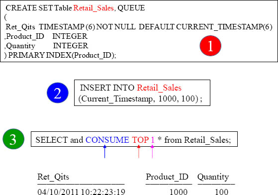
This row will automatically be DELETED because of our SELECT and CONSUME TOP 1 Statement. That is the purpose of a QUEUE table. You set it up so it can process rows one at a time and then delete them.
Column Attributes
UPPERCASE - Convert and store entered data in uppercase
CASESPECIFIC - Treat data as case specific for all comparisons
FORMAT - Establishes the display format
TITLE - Establishes the title attribute
NAMED - Establishes an alias name
WITH DEFAULT - Default numeric values to zero, characters values to blanks
DEFAULT DATE - Use today’s date as default value
DEFAULT TIME - Use current time as default value
COMPRESS - Compress nulls to take no disk space.
COMPRESS NULL - Compress nulls to take no disk space
COMPRESS <data-value> - Compress specified value(s) to take no disk space, value(s) stored in the table header.
CHARACTER SET - Establishes the computer internal storage rules and how it should be interpreted. i.e. LATIN and KANJI
NOT NULL - Disallow nulls to be stored in the column
GENERATED BY - System generated value for the column, specifies the increment
DEFAULT Value - Use default value if null entered
DEFAULT User - Use the user’s ID as the default value for the column
DEFAULT AS IDENTITY - Use generate a unique value for this column
DEFAULT NULL - Use null as the default value for the column
When defining a table it is normally advantageous to be more specific regarding the definition of the columns and their attributes. These attributes are listed above.
An Example of a Table With Column Attributes
CREATE Table Employee_Attr
(emp |
INTEGER |
,dept |
INTEGER NOT NULL |
,lname |
CHAR(20) NOT CASESPECIFIC |
,fname |
VARCHAR(20) TITLE 'FIRST NAME' |
,salary |
DECIMAL(10,2) FORMAT 'ZZ,ZZZ,ZZ9.99' |
,hire_date |
DATE FORMAT 'mmmBdd,Byyyy' |
,Byte_col |
BYTE(10) compress '000000'xb ) |
UNIQUE PRIMARY INDEX(emp);
In the above example the columns have been further defined using column attributes. The dept column is defined with the NOT NULL attribute. This means that a NULL value cannot be stored in the dept column. The lname column has been further defined to state that for comparison purposes, the data is not case specific. This means that it does not matter if the data is in upper case, lower case, or a combination. The fname column has a TITLE associated with it. So, whenever it is selected, ‘FIRST NAME’ appears as the report heading instead of the column name. The salary column is automatically formatted as currency in the output when selected using BTEQ. The hire_date is also formatted. It displays as the alpha month followed by the numeric day and 4-digit year. Lastly, the Byte_Col column is added. It is a byte column with a length of 10. The example shows how to initialize it with a value of zero. It is provided as a hexadecimal number using the xb designation. This designation would also be a valid comparison for retrieval of the row. Notice the word compress.
An Example of a Table With Column Level Constraints
CREATE Table Employee_Col_Constr
( emp INTEGER NOT NULL
CONSTRAINT EmpPK PRIMARY KEY
,dept INTEGER CONSTRAINT Ref_1 REFERENCES
Department(dept) BETWEEN 10 AND 100
,lname CHAR(20) NOT NULL
,fname VARCHAR(20) NOT NULL
,salary DECIMAL(10,2) CONSTRAINT SalCheck
CHECK (salary >=10000 and salary < 1000000)
,hire_date DATE
,soc_sec INTEGER NOT NULL
CONSTRAINT SSNUniq UNIQUE ) ;
In the above table, the emp column must have a value because it cannot be null. It also has a primary key named EmpPK and therefore, becomes the UPI of this table because no Primary Index was explicitly defined. The dept column has an RI constraint named Ref_1 on the column called dept in the Department table. This means that a dept cannot be entered into the employee table unless that dept exists in the department table. This is referential integrity as its best! There is a CHECK constraint called SalCheck on the salary column and it requires the salary to be at least $10,000.00 up to a maximum of $99,999.99. The last two constraints are on the soc_sec column. First, there is the NOT NULL that requires a value to be stored there. Then, the SSNUniq constraint requires that the value be different from any other value in other rows because it must be unique.
An Example of a Table With Table Level Constraints
CREATE Table Employee_Constr2, FALLBACK
(emp INTEGER GENERATED BY DEFAULT AS IDENTITY
NOT NULL
,dept INTEGER
,lname CHAR(20) NOT NULL
,fname VARCHAR(20) NOT NULL
,sal DECIMAL(10,2)
,hire_date DATE
,soc_sec INTEGER NOT NULL,
CONSTRAINT EmpPK PRIMARY KEY (emp),
CONSTRAINT Ref_1 FOREIGN KEY (dept)
REFERENCES Department(dept),
CONSTRAINT NameUniq UNIQUE (lname, fname),
CONSTRAINT Sal_Dept_Check CHECK
(sal >= 10000 AND sal < 100000
AND dept BETWEEN 10 AND 100),
CONSTRAINT SSNUniq UNIQUE (soc_sec) ) ;
We feel this type of definition is easier to read and understand than looking for constraints throughout the DDL. These constraints are all the same as in the first example, with one exception. Here, the name constraint called NameUniq uses a combination of both the fname and the lname columns to create a USI. Notice too that NOT NULL must still be at the column level. Also notice that the emp column now is a system generated number. Anytime an INSERT is requested and a null value is assigned to the column, it generates a consecutive number, one greater than the value assigned previous row. The difference between BY DEFAULT and ALWAYS is that DEFAULT only generates the number when a null is received. Otherwise, the value provided in the INSERT is used for the column. On the other hand, the ALWAYS generates the number even when a value is present for the column.
Create Table AS

Above are some great examples to quickly CREATE a Table from another table. Our third example errors.
Creating Partitioned Primary Index (PPI) Volatile Tables
CREATE VOLATILE TABLE Order_PPI
AS ( SELECT * FROM Order_Table
WHERE Order_Date BETWEEN
DATE '2013-01-01' and '2013-06-30')
WITH DATA
PRIMARY INDEX (Order_Number)
PARTITION BY RANGE_N( ORDER_DATE
BETWEEN Date '2013-01-01' and Date '2013-06-30'
EACH INTERVAL '1' DAY) ;
Above you can see an example of quickly creating a Partitioned table directly from the actual Order_Table. We only inserted some of the data with our WHERE clause and we partitioned by day.
A Volatile Table That Only Populates Some of the Rows
Create a Table with orders from September
CREATE TABLE Order_Vol
AS (SELECT * FROM Order_Table
WHERE Extract(Month from Order_Date) = 9)
WITH DATA PRIMARY INDEX (Customer_Number) ;
Above is an example of creating a table that is not an exact copy. It is only populating the table with orders from the month of September.
A Volatile Table With No Data
This creates a table with no data
CREATE TABLE Order_Empty
AS (SELECT * FROM Order_Table)
WITH NO DATA
PRIMARY INDEX(Customer_Number);
You must have either
WITH DATA
or
WITH NO DATA
INSERT INTO Order_Empty
SELECT * FROM SQL_Class.Order_Table ;
Above is an example of creating a table with no data. This must be further populated with an Insert/Select.
A Volatile Table With Some of the Columns
This creates a table with only three columns
CREATE TABLE Order_Vol5
AS (SELECT Customer_Number
,Order_Date, Order_Total
FROM Order_Table)
WITH DATA ;
Above is an example of creating a table with three columns. The original table had four columns.
A Volatile Table With No Data and Zeroed Statistics
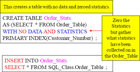
Collect Statistics ON Order_Stats ;
The same statistics (columns/indexes) from the Order_Table are now recollected for the Order_Stats table
Above is an example of creating a table with no data and zeroed statistics. This must be further populated with an Insert/Select. Since the new table had no data and statistics the statistics are all set to zero. When the table is populated with an Insert/Select it now has data. When the Collect Statistics command is run the same statistics that were collected on the Order_Table will be recollected on the new table. That is the purpose of zeroed statistics.
A Multiset Volatile Table With Statistics Example

Above is an example of creating a table that is a Multiset table. A Multiset table allows duplicate rows, but a Set table deletes any rows that are duplicated in their entirety. It also brings over the statistics from the Order_Table.
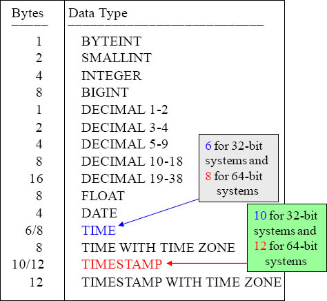
Data Types

Data Types Continued

Data Types Continued

Major Data Types and the number of Bytes they take up