CHAPTER 7

Cost–Volume–Profit Relationships

This chapter examines how a company’s cost structure impacts its profitability as various activities that drive cost change in volume. The process by which these relationships are examined is referred to as cost–volume–profit analysis, or CVP analysis.

The term cost structure pertains to how a company’s total costs are divided between costs that are fixed (those that do not change significantly as business activities change), and costs that are variable (those that do change measurably as business activities change). CVP analysis focuses upon business activities that are highly correlated with driving up a company’s costs and identifies these activities as cost drivers. Throughout this chapter, units produced and sold will be the primary cost driver used to illustrate CVP relationships.¹

CVP analysis is a valuable planning tool that can be used by managers to address questions related to:

• The number of units a company must sell in order to break even;
• The dollar amount of sales needed to achieve a target level of income;
• The amount by which current sales levels can decline before a company becomes unprofitable;
• The amount by which a company’s profitability will change if its current sales mix changes, and so on.

Cost Behaviors

CVP analysis requires that managers classify costs as being either variable or fixed.² Variable costs vary in total as business activity varies, but on a per unit basis, they remain fixed. For instance, if the cost of producing a product includes $10 per unit in raw material, total material costs increase as the number of units produced increases; however, the material cost per unit remains fixed at $10.³ The graphs in Figure 7.1 illustrate variable cost behavior.

Figure 7.1 Variable cost behavior

Fixed cost behavior is the mirror image of variable cost behavior. Fixed costs are generally fixed in total across a normal range of activity, but vary per unit as activity varies. For example, assume that a company’s monthly fixed costs remain relatively constant at $5,000 across a normal range of production activity between 1,000 units and 5,000 units. So, if 1,000 units are produced, the average fixed cost per unit will be $5 ($5,000 ÷ 1,000 units), but if 5,000 units are produced, the average fixed cost per unit will be just $1 ($5,000 ÷ 5,000 units). Thus, fixed costs could be as high as $5 per unit or as low as $1 per unit, which demonstrates that assigning fixed costs to products or services on a per unit basis is like trying to measure the cost of something using a rubber ruler. Consequently, CVP analysis always considers fixed costs in the aggregate to avoid having unit costs vary as output activity varies. The graphs in Figure 7.2 illustrate fixed cost behavior.

Figure 7.2 Fixed cost behavior

Contribution Income Statements

Income statements prepared for external users under generally accepted accounting principles (GAAP) assign costs and expenses to both products and reporting periods. Costs assigned to products are reported in the income statement as cost of goods sold, whereas costs that are more broadly assigned to reporting periods appear in the income statement as operating expenses—such as salaries, insurance, marketing costs, and legal fees. This approach to classifying costs does not work for CVP analysis because product and period costs reported under GAAP include both fixed and variable cost elements.⁴

For internal (managerial) purposes, income statements are often rearranged into what is referred to as a contribution format.⁵ Figure 7.3 provides a side-by-side illustration of income statements prepared under GAAP and contribution formats. It is important to note that both formats report the same dollar amount of operating income.⁶

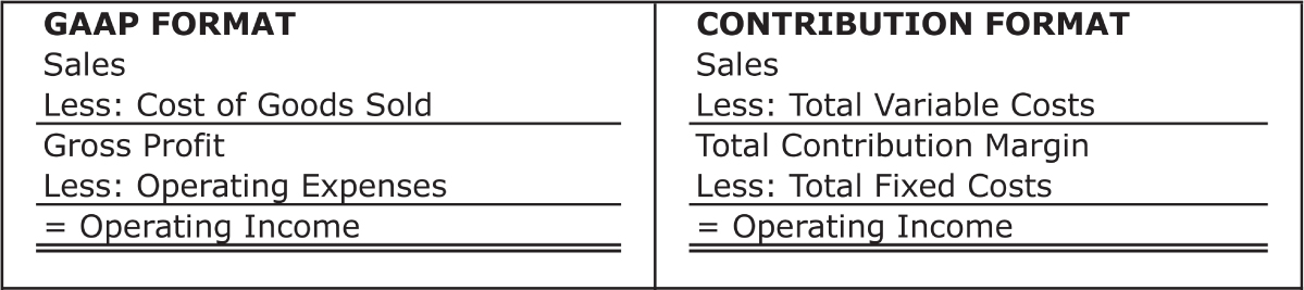
Figure 7.3 Income statements: GAAP versus contribution formats

Unlike the GAAP format—in which cost of goods sold and operating expenses include both fixed and variable cost elements—the contribution format classifies costs as being either variable or fixed, of which both classifications include elements of cost of goods sold and operating expenses. Notice that under the contribution format total contribution margin is used as a subtotal instead of gross profit. The concept of contribution margin is central to CVP analysis and it will be addressed later in this chapter.

Finally, both income statement formats presented in Figure 7.3 conclude with operating income instead of net income. Operating income—income before deducting income tax expenses—is used more frequently in CVP analysis than net income because income taxes behave neither like variable costs nor like fixed costs. Income taxes are legislated, so they often behave in ways that defy logic.⁷

The Cost–Volume–Profit Graph

It is helpful to graph the elements of CVP relationships before engaging in the process of CVP analysis. Figure 7.4 illustrates these important CVP relationships.

Figure 7.4 Cost–volume–profit relationships

The horizontal axis of the graph represents the number of units that a company produces and sells, whereas the vertical axis is expressed in dollars.⁸ The total fixed cost line is parallel to the horizontal axis, indicating that total fixed costs remain constant over a normal range of units produced and sold. The total cost line is composed of fixed costs plus variable costs. It originates where the total fixed cost line meets the vertical axis. Hypothetically, with no production or sales activity, variable costs would be zero, and total costs would simply be a company’s total fixed costs. With each additional unit produced and sold, a company’s total cost goes up by the variable cost per unit—which means that the slope of the total cost line equals the variable cost per unit. Thus, the formula for total cost line can be expressed as follows:

Total Costs = Total Fixed Costs + (Units Produced & Sold × Variable Cost per Unit)

The total sales revenue line begins at the graph’s origin, and with each additional unit produced and sold, total sales revenue increases by the selling price per unit. Thus, the slope of the total sales revenue line equals the selling price per unit.

Initially, the graph’s total cost line is above the total sales revenue line, meaning that the company is unprofitable and operating at a loss. Where the total cost and total sales revenue lines intersect is the breakeven point (which is measured in sales dollars on the vertical axis and in units produced and sold on the horizontal axis). At the breakeven point the company’s income equals zero. Beyond the breakeven point, the graph’s total sales revenue line is above the total cost line, meaning that the company is operating at a profit.

Contribution Margin Per Unit

The amount by which the slope of the total sales revenue line (selling price per unit) exceeds the slope of the total cost line (variable cost per unit) is referred to as the contribution margin per unit. Thus, the contribution margin per unit is computed as follows:

Contribution Margin/Unit = Unit Selling Price – Unit Variable Cost

Assume, for example, that a company makes a single product with a selling price of $100 and a variable cost per unit of $60. Thus, its contribution margin per unit is $40. This means that up to the breakeven point each unit produced and sold contributes $40 toward covering the company’s total fixed costs. After the breakeven point, each unit produced and sold contributes $40 to the company’s operating income. If the company’s monthly fixed costs total $6,000, it must produce and sell 150 units to break even, computed as follows:

$6,000 total fixed costs ÷ $40 contribution margin per unit = 150 units to breakeven

It is not uncommon to express the contribution margin per unit as a percentage of the selling price per unit. The result is referred to as the contribution margin percentage. If the selling price is $100, and its contribution margin per unit is $40, then its contribution margin percentage is 40 percent, computed as follows:

$40 contribution margin per unit ÷ $100 unit selling price = 40% contribution margin percentage

CVP Formulas

The contribution margin per unit and the contribution margin percentage are key variables in two CVP formulas used to determine the level of sales activity required—in units or in dollars—to achieve a target level of operating income. The two formulas are provided in Figure 7.5. The manner in which these formulas are used is illustrated throughout the remainder of this chapter.

Figure 7.5 Sales volume required for target operating income

The Case of Splash Enterprises—Part I

Splash Enterprises manufactures and sells ski vests used by water skiers and boaters. It currently sells no other products. A summary of the company’s unit selling price, unit variable cost, monthly fixed costs, contribution margin, and contribution margin percentage is provided in Figure 7.6.

Figure 7.6 CVP analysis in a single product environment

Using the information in Figure 7.6 with the CVP formulas in Figure 7.5 enables Splash’s management team to better understand important relationships involving the company’s cost structure, its volume of sales activity, and its profitability.

What Is Splash’s Monthly Breakeven Point in Units?

As mentioned previously, the breakeven point is reached when a company’s total sales revenue equals its total costs. At the breakeven point operating income equals zero. Thus, using the first CVP formula shown in Figure 7.5, Splash’s monthly breakeven point in units is estimated as follows:

Sales in Units = [Fixed Costs + Target Operating Income] ÷ Contribution Margin/Unit

Sales in Units = [$270,000 + $0] ÷ $90

Sales in Units = 3,000 Units

In short, if Splash sells fewer than 3,000 ski vests in any given month, it will report an operating loss; however, each ski vest produced and sold in excess of 3,000 units will contribute $90—the contribution margin per unit—to the company’s monthly operating income.

What Is Splash’s Monthly Breakeven Point in Dollars?

Again, operating income equals zero at the breakeven point, so using the second CVP formula shown in Figure 7.5, the company’s monthly breakeven point in dollars is estimated as follows:

Sales in Dollars = [Fixed Costs + Target Operating Income] ÷ Contribution Margin%

Sales in Dollars = [$270,000 + $0] ÷ 60%

Sales in Dollars = $450,000

To avoid an operating loss, Splash needs to generate monthly sales revenue of at least $450,000. After the breakeven point is reached, each dollar of sales revenue in excess of $450,000 will contribute $0.60—the contribution margin percentage—to the company’s monthly operating income.⁹

It is easy to see that fixed costs directly impact a company’s ability to break even. The more a company’s cost structure is composed of fixed costs—relative to variable costs—the more difficult it becomes for it to break even. For instance, if Splash’s fixed costs increase by $90,000—from $270,000 to $360,000—its level of sales required to break even will increase by $150,000—from $450,000 to $600,000—and its breakeven point will increase from 3,000 units to 4,000 units.¹⁰

Beyond the Breakeven Point

It would not make sense for a company to establish the breakeven point as its target performance objective. The breakeven point is determined simply to ascertain the sales level required (in units or in dollars) to cover total fixed costs. The more important issue that confronts managers is how profit changes in response to sales once the breakeven point has been reached. Understanding how cost structure affects profitability enables managers to estimate the sales volumes necessary to achieve profitability targets beyond the breakeven point.

In May, Splash’s management team set a target operating income of $72,000 for June. Historically, the average operating income in June has been $63,000. How many ski vests must Splash sell to achieve its target? The answer to that question can be quickly determined using the first CVP formula shown in Figure 7.5:

Sales in Units = [Fixed Costs + Target Operating Income] ÷ Contribution Margin/Unit

Sales in Units = [$270,000 + $72,000] ÷ $90

Sales in Units = 3,800 Units

Using the second CVP formula shown in Figure 7.5, the dollar level of sales required for Splash to achieve its June target is:

Sales in Dollars = [Fixed Costs + Target Operating Income] ÷ Contribution Margin%

Sales in Dollars = [$270,000 + $72,000] ÷ 60%

Sales in Dollars = $570,000

Given that Splash’s average operating income in June is $63,000, by how much can the company’s sales revenue (in dollars) decline before it becomes unprofitable? CVP analysis makes the answer to this question easy to determine. Using the second CVP formula shown in Figure 7.5, the dollar level of sales required for Splash to achieve June’s average operating income of $63,000 is determined as follows:

Sales in Dollars = [Fixed Costs + Target Operating Income] ÷ Contribution Margin%

Sales in Dollars = [$270,000 + $63,000] ÷ 60%

Sales in Dollars = $555,000

Splash’s sales revenue (in dollars) required to break even was determined previously as $450,000. Should sales decline below this amount, the company will be unprofitable. Thus, the $555,000 average sales revenue in June can decline by $105,000 before Splash incurs an operating loss. The amount by which a company’s current sales level can decline before it becomes unprofitable is referred to as its margin of safety. In this case, Splash’s margin of safety is $105,000.¹¹

What about Taxes?

Up to this point, CVP analysis has been illustrated using operating income instead of after-tax income. What if Splash wants to estimate sales activity to achieve a target after-tax income? Dividing the after-tax income target by one minus the company’s average tax rate, and using that result in the Figure 7.5 formulas, enables CVP analysis to be used for after-tax estimates.

For instance, assume that Splash’s average tax rate is 25 percent, and that management wants to determine the sales revenue required (in dollars) for an after-tax profit of $45,000. One minus the company’s average tax rate of 25 percent equals 75 percent, and $45,000 after-tax profit divided by 75 percent equals $60,000. Using this figure as the income target in the second CVP formula shown in Figure 7.5, the dollar level of sales required for Splash to achieve an after-tax profit of $45,000 is derived as follows:

Sales in Dollars = [Fixed Costs + (After-Tax Income)/(1 − Tax Rate)] ÷ Contribution Margin%

Sales in Dollars = [$270,000 + ($45,000/75%)] ÷ 60%

Sales in Dollars = [$270,000 + $60,000] ÷ 60%

Sales in Dollars = $550,000

As noted previously, income taxes do not behave like variable costs, nor do they behave like fixed costs. Income taxes are legislated, and they often behave in ways that defy logic. As such, it is common for managers to use operating income—instead of after-tax income—when performing CVP analysis.

The Case of Splash Enterprises—Part II

In the previous section, Splash produced and sold ski vests as its only product. Of course, many companies sell hundreds or even thousands of different products. So the obvious question is whether CVP analysis applies to multiple product environments. The answer to that question is yes, but with some adjustments. The complexity of applying CVP increases as product lines increase; however, the underlying conceptual issues of most importance are pretty much the same across an array of multiple product environments.

To illustrate, assume that Splash decides to diversify its offerings to include life vests, slalom skis, and ski ropes. Information pertaining to its expanded line of products is provided in Figure 7.7.

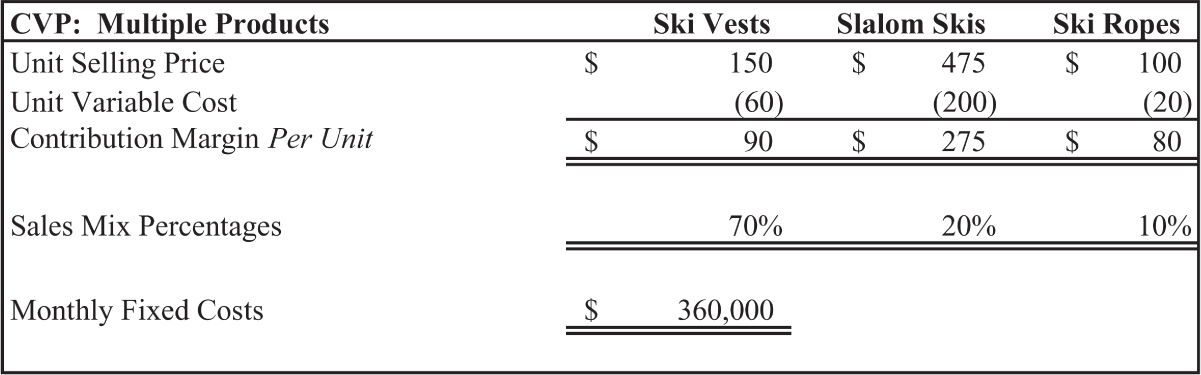
Figure 7.7 CVP analysis in a multiple product environment

As indicated, the company’s ski vests sell for $150 apiece, provide a contribution margin of $90 per unit, and account for approximately 70 percent of the company’s total sales revenue. Slalom skis sell for $475 apiece, offer a contribution margin of $275 per unit, and account for 20 percent of the company’s total sales revenue. Ski ropes (with all of their necessary hardware) sell for $100 apiece, have a contribution margin of $80 per unit, and account for the remaining 10 percent of the company’s total sales revenue.¹² The decision to produce and sell multiple product lines increased Splash’s monthly fixed costs from $270,000 to $360,000.

Now that Splash sells more than one product, expressing its sales activity in total unit sales is less meaningful than expressing its sales activity in total dollars of sales revenue. For this reason, multiproduct companies generally use CVP analysis only for determining the total dollars of sales revenue necessary to achieve operating income targets.

Recall that in a single product environment, determining sales levels in dollars was computed using the contribution margin percentage in the following CVP formula introduced in Figure 7.5:

Sales in Dollars = [Fixed Costs + Target Operating Income] ÷ Contribution Margin%

In a single product environment, the contribution margin percentage is the product’s contribution margin per unit divided by its selling price per unit. In a multiproduct environment, every product has a unique contribution margin and selling price. Thus, determining sales levels in dollars requires a weighted-average contribution margin percentage (WACM%). The WACM% is computed by dividing a company’s weighted-average contribution margin (WACM) by its weighted-average selling price (WASP).

The computation of Splash’s WACM% is provided in Figure 7.8. In the top half of Figure 7.8, Splash’s WACM of $126 was computed by multiplying each product’s contribution margin by its sales mix percentage, and summing the results across all product lines. In the bottom half of Figure 7.8, the company’s WASP of $210 was computed by multiplying each product’s selling price by its sales mix percentage, and summing the results across all products. Thus, Splash’s WACM% (WACM ÷ WASP) is 60 percent ($126 ÷ $210), which can be used to modify CVP formula introduced in Figure 7.5 by substituting it in the denominator, as shown below:

Figure 7.8 Weighted-average contribution margin percentage

Sales in Dollars = [Fixed Costs + Target Operating Income] ÷ WACM%

Using this modified formula, CVP analysis is no more difficult than when Splash sold only life vests—assuming that its sales mix percentages remain relatively constant.

What Is Splash’s Monthly Breakeven Point in Dollars?

At the breakeven point, operating income is zero. Thus, its breakeven point in sales dollars is:

Sales in Dollars = [Fixed Costs + Target Operating Income] ÷ WACM%

Sales in Dollars = [$360,000 + $0] ÷ 60%

Sales in Dollars = $600,000

So long as Splash’s sales mix percentages remain relatively constant, it needs to generate monthly sales revenue of at least $600,000 to avoid an operating loss. Once the breakeven point is reached, each dollar of sales revenue in excess of $600,000 will contribute $0.60—the WACM%—to the company’s monthly operating income.

Achieving Operating Income Targets

Assume that Splash’s management has set an operating income target of $150,000 for the upcoming month. Applying the same formula that was used to determine the company’s breakeven point, the sales dollars required to achieve its target operating income can be estimated as follows:

Sales in Dollars = [Fixed Costs + Target Operating Income] ÷ WACM%

Sales in Dollars = [$360,000 + $150,000] ÷ 60%

Sales in Dollars = $850,000

If this target is achieved, Splash’s margin of safety—the amount by which its sales can decline before it becomes unprofitable—will be $250,000 (the target sales revenue of $850,000, minus the breakeven sales revenue of $600,000).

Achieving After-Tax Income Targets

Had Splash’s target income for the upcoming month been $180,000 expressed as an after-tax amount, the same approach that was used in the single product illustration can be applied. If the company’s tax rate is 25 percent, the required sales in dollars can be estimated by dividing the target after-tax income by 75 percent (one minus the tax rate), and by substituting the WACM% in the denominator, as shown below:

Sales in Dollars = [Fixed Costs + (After-Tax Income)/(1 − Tax Rate)] ÷ WACM%

Sales in Dollars = [$360,000 + ($180,000/75%)] ÷ 60%

Sales in Dollars = [$360,000 + $240,000] ÷ 60%

Sales in Dollars = $1,000,000

Managing Sales Mix Percentages

Managers often try to improve profitability by shifting the sales mix away from products with the lowest contribution margin percentages to those with the highest contribution margin percentages. This strategy is sometimes referred to as improving the quality of sales.

Ski vests account for 70 percent of Splash’s sales revenue and have a contribution margin percentage of 60 percent ($90 per unit contribution margin ÷ $150 unit selling price). Slalom skis account for 20 percent of the company’s sales revenue and have a 57.9 percent contribution margin percentage ($275 unit contribution margin ÷ $475 selling price). Thus, Splash would not benefit from efforts to shift its sales mix away from ski vests to sales of slalom skies. Ski ropes account for only 10 percent of the company’s sales revenue; however, they generate a contribution margin percentage of 80 percent ($80 per unit contribution margin ÷ $100 selling price). As such, Splash may wish to explore marketing efforts that would increase the percentage of its total sales revenue that it generates from ski ropes.

Summary

This chapter examined the impact of cost structure on a company’s profitability as business activity changed in volume.¹³ The process by which these relationships were examined was referred to as CVP analysis. Throughout the chapter CVP analysis was used to graph cost behaviors, determine breakeven points, compute sales volume needed to achieve target incomes, quantify margins of safety, and to better understand a variety of other issues related to a company’s cost structure.

CVP analysis is a powerful managerial tool; however, CVP formulas are based on several fairly rigid assumptions. For instance, increases in total sales revenue and total costs are considered linear over a normal range of activity, whereas total fixed costs are assumed to remain constant as activity levels change. For companies that sell multiple product lines, sales mix percentages are assumed to be constant in the short run, and for manufacturing companies, units produced are assumed to equal units sold.

Even though CVP analysis is a fairly straightforward endeavor, even the simplest CVP models must be flexible and interactive so that inputs to the process can be adjusted efficiently as assumptions about the future change. Thus, CVP analysis is almost always performed using Excel or cost accounting software. In fact, CVP relationships often are built into robust forecasting models similar to those examined in Chapters 5 and 6.

____________

¹Many different kinds of activities can be cost drivers. For instance, in large-scale manufacturing operations, machine hours are often correlated highly with cost incurrence, whereas in small companies that create handcrafted products—such as custom furniture—labor hours can be a significant cost driver. In the airline industry, the number of passenger miles flown is commonly considered a primary cost driver, and in hospitals, the number of inpatient-days is widely used. Many companies use multiple cost drivers when performing CVP analysis; moreover, they apply CVP at various organizational levels including divisions, departments, and individual products.

²Some costs are semivariable—or mixed—meaning that they contain both variable and fixed elements. For instance, electricity costs are usually composed of a fixed monthly rate plus a variable amount based on the number of kilowatt hours used.

³CVP analysis applies to normal ranges of activity. Should activities—such as production levels—fall outside of normal ranges, variable costs per unit can change as economies of scale change. If activity falls below normal, economies of scale can be lost, causing variable costs per unit to increase. Likewise, if activity exceeds what is normal, economies of scale can be gained, causing variable costs per unit to decrease.

⁴This is especially true of manufacturing environments, where cost of goods sold includes large amounts of fixed overhead costs incurred in the production process.

⁵Income statements prepared under the contribution format are also referred to as variable costing income statements.

⁶In manufacturing environments, operating income can differ between the two formats if a company’s ending inventory differs materially from its beginning inventory. The difference stems from the manner in which fixed manufacturing costs are accounted for under GAAP—a topic beyond the scope of this book.

⁷Using after-tax income in CVP analysis will be illustrated later in this chapter.

⁸Labeling the horizontal axis as units produced and sold suggests that the graph is for a manufacturing company. A wholesaler or retailer might label the horizontal axis as units sold. The horizontal axis used in a CVP graph needs to be a business activity that is highly correlated with a company’s total cost. As discussed previously, business activities that are highly correlated with costs are called cost drivers. Depending on the type of business being analyzed, cost drivers might also include machine hours, labor hours, passenger miles traveled, inpatient days, and so on.

⁹The same $450,000 breakeven sales figure could have been derived by multiplying the company’s breakeven point in units by the selling price per ski vest: 3,000 units × $150 per ski vest = $450,000.

¹⁰Breakeven computations if fixed costs increase to $360,000: [$360,000 + $0] ÷ 60% = $600,000; [$360,000 + $0] ÷ $90 = 4,000 units.

¹¹Splash’s margin of safety also can be stated as 700 units ($105,000 margin of safety ÷ $150 selling price per unit = 700 units). Thus, average sales in June could fall by 700 units before Splash would report a monthly operating loss.

¹²The sales mix percentages shown in Figure 7.7 refer to how much each product contributes to the total sales revenue generated by the entire company. Thus, ski vests provide 70 percent of the company’s total sales revenue, whereas ski ropes provide only 10 percent.

¹³CVP focuses exclusively on the relationship between cost structure and profitability; it is not used to analyze relationships that exist between a company’s cost structure and its cash flow.