
In this chapter we review the problem faced by government in adjusting monetary and fiscal policy to the underlying conditions relating to the labor market and the growth of real GDP. There are, to be sure, many goals to which macroeconomic policies can, and should, be applied. Among them are price stability, economic growth, exchange rate stability, and some measure of equity, among others. Here we focus on the problem of calibrating monetary and fiscal policy to keep real GDP at its full-employment level.1
Consider Figure 4.1, also seen in the previous chapter. In Volume I, we considered how tax policy affects the point at which the LRAS line cuts the horizontal axis, shown as point A in Figure 4.1. Reductions in tax rates and welfare benefits (and generally, the elimination of government-imposed distortions in the price system) shift the LRAS curve to the right. The opposite policies shift it to the left.
In Chapter 3 of this volume we reviewed the circumstances under which actual output, Y, deviates from full-employment output, YFE. In the short run, a rise or fall in aggregate demand can cause actual Y to exceed or fall below YFE. What happens to Y depends on whether workers or employers misread the change in aggregate demand as an event localized to their particular portion of the market, when in fact it is an economywide event. If there is myopia, wages will lag behind prices in adjusting to a fall or rise in aggregate demand, causing Y to fall temporarily below, or temporarily rise above, YFE.
If Y is below YFE, the problem will be self-correcting if workers or employers come to understand that what they saw as a localized change in demand is, in fact, an economywide change. It will be self-correcting if caught early enough. It will not be self-correcting if it leads to an irreversible shrinkage in employment opportunities or worker availability. If aggregate demand falls and if wages do not both fall by the same rate as prices, the layoffs that result will bring about a spiraling reduction in demand for goods and labor. If aggregate demand rises and if wages don’t rise by the same rate as prices, the worker departures from the labor force that result will bring about a spiraling reduction in the supply of goods and labor.

Figure 4.1 Long-run equilibrium price and output
This means that policymakers have three problems to solve. The first is whether and how to eliminate distortions in the price system that reduce YFE. The second is to determine whether at any time Y has fallen below YFE and, if so, whether the fall is self-correcting or (quasi) permanent. Then if that problem is not self-correcting, the third problem is deciding how to use the policy instruments at its disposal to increase or to decrease aggregate demand.
Neither workers nor employers have a monopoly on their inclination to misdiagnose a change in aggregate demand. Government can as well misdiagnose a fall in output and employment and, when it does, it might provide a remedy opposite of what is called for. The most likely misdiagnosis, given the Keynesian bias that runs through policy making and analysis, is to misinterpret a fall in aggregate supply as a fall in aggregate demand. The government might, for example, offer more generous social benefits to correct a problem aggravated by an increase in social benefits.
In this chapter, we generalize conclusions of the preceding chapter to account for how policymakers adjust their actions to changes in the growth of real GDP and to labor market indicators, particularly the unemployment rate.
Let’s assume that the policy goal is to increase YFE to the degree that is politically feasible and then to keep Y as closely aligned with YFE as possible.
We begin again with the equation,
![]()
Now let’s think of how we have to adjust this equality to reflect growth in each of the variables. We can write
![]()
![]()
which implies that the percentage change in M will, by necessity, equal the percentage change in k plus the percentage change in P plus the percentage change in Y. There must be a match between the growth of the supply of money (the left-hand side of the equation) and the growth of the demand for money (the right-hand side of the equation). The question for monetary policy is how to calibrate ![]() , given the sensitivity of
, given the sensitivity of ![]() ,
, ![]() , and
, and ![]() to
to ![]() . Chapter 1 of this volume outlined the options available to the Federal Reserve System policy in addressing this problem. If k is constant, we can interpret the equation to say that a change in the growth of M requires a commensurate change in the growth of PY.
. Chapter 1 of this volume outlined the options available to the Federal Reserve System policy in addressing this problem. If k is constant, we can interpret the equation to say that a change in the growth of M requires a commensurate change in the growth of PY.
Let’s use the symbol ![]() normal to represent the normal growth rate of real GDP, Y. We saw in Volume I, Chapter 6 that there would be some normal growth of Y in an economy where the growth of Y just matches the growth of the number of workers, L (assuming that Z is constant). Say, for example, that we expect L to grow by 3% annually, so that expected
normal to represent the normal growth rate of real GDP, Y. We saw in Volume I, Chapter 6 that there would be some normal growth of Y in an economy where the growth of Y just matches the growth of the number of workers, L (assuming that Z is constant). Say, for example, that we expect L to grow by 3% annually, so that expected ![]() =
= ![]() normal = 3%. Now let’s also suppose that there is some targeted inflation rate,
normal = 3%. Now let’s also suppose that there is some targeted inflation rate, ![]() targeted = 2%. Then, in order to maintain full employment, the growth of the nominal wage rate
targeted = 2%. Then, in order to maintain full employment, the growth of the nominal wage rate ![]() must be 2% so that the real wage rate remains constant. This assumes that the volume of labor services, L, is growing in tandem with Y, so that there is no change in labor productivity Y/L. Given that
must be 2% so that the real wage rate remains constant. This assumes that the volume of labor services, L, is growing in tandem with Y, so that there is no change in labor productivity Y/L. Given that ![]() is zero, we can use equation (4.3) to solve for the required growth in M:
is zero, we can use equation (4.3) to solve for the required growth in M:
![]()
By this logic (and assuming that k is constant), the required annual growth of the money supply equals the normal annual growth of real GDP (which for many years in the United States, was about 3%) plus the targeted rate of inflation.
If ![]() =
= ![]() normal, real GDP (Y) equals the full-employment real GDP, YEF. The size of L depends on the unemployment rate, UR, and the labor force participation rate, LFPR: If
normal, real GDP (Y) equals the full-employment real GDP, YEF. The size of L depends on the unemployment rate, UR, and the labor force participation rate, LFPR: If ![]() =
= ![]() normal, everyone in the age-eligible population who wants to work will be in the labor force. Everyone in the labor force will have a job except for temporary mismatches owing to “frictional” or “structural” factors.
normal, everyone in the age-eligible population who wants to work will be in the labor force. Everyone in the labor force will have a job except for temporary mismatches owing to “frictional” or “structural” factors.
When ![]() =
= ![]() normal, the resulting unemployment rate is called the natural rate of unemployment or, more descriptively, the nonaccelerating inflation rate of unemployment (or NAIRU). This is the rate of unemployment that exists when nominal wages are changing in tandem with prices so as to maintain equality between
normal, the resulting unemployment rate is called the natural rate of unemployment or, more descriptively, the nonaccelerating inflation rate of unemployment (or NAIRU). This is the rate of unemployment that exists when nominal wages are changing in tandem with prices so as to maintain equality between ![]() =
= ![]() normal.
normal.
The unemployment rate falls below the NAIRU when prices rise faster than wages and when workers expand their work effort even though their real wages are falling. We can coin an analogous term to represent the rate of labor force participation when wages are changing at the same rate as prices. Let’s call that rate the nonaccelerating inflation rate of labor-force participation or NAPR (ugly, true, but not much worse than NAIRU). NAPR is the labor-force participation rate that exists when nominal wages are changing at the same rate as prices and when they are both changing just fast enough to keep ![]() =
= ![]() normal. The labor-force participation rate falls below the NAPR when myopic employers keep
normal. The labor-force participation rate falls below the NAPR when myopic employers keep ![]() below
below ![]() > 0 and when people leave the labor force as a result.
> 0 and when people leave the labor force as a result.
Full employment is the level of employment that exists when the unemployment rate and the labor-force participation rate are both at their “natural” or “nonaccelerating” levels. Such unemployment, if it exists, is frictional or structural in nature but not the result of any imbalance between aggregate supply and demand.
The Phillips Curve
Consider now a scenario in which the growth of the money supply rises so that, temporarily,
![]()
If the economy is at full employment and if prices and wages rise at the same rate as M, ![]() will equal to
will equal to ![]() normal. But suppose that
normal. But suppose that ![]() lags behind
lags behind ![]() , causing the cost of labor to fall. Suppose also that myopic workers, confusing the rise in nominal wages with a rise in real wages, expand their work effort. Then
, causing the cost of labor to fall. Suppose also that myopic workers, confusing the rise in nominal wages with a rise in real wages, expand their work effort. Then ![]() will temporarily rise above
will temporarily rise above ![]() normal, and the unemployment rate will fall below the NAIRU. Laurence Ball and N. Gregory Mankiw say that “there is wide agreement about the fundamental insight that monetary fluctuations push inflation and unemployment in opposite directions. That is, society faces a tradeoff, at least in the short run, between inflation and unemployment” (Ball and Mankiw 2002, p. 116).
normal, and the unemployment rate will fall below the NAIRU. Laurence Ball and N. Gregory Mankiw say that “there is wide agreement about the fundamental insight that monetary fluctuations push inflation and unemployment in opposite directions. That is, society faces a tradeoff, at least in the short run, between inflation and unemployment” (Ball and Mankiw 2002, p. 116).
This relationship is known as the Phillips curve, as shown in Figure 4.2. There we draw a short-run Phillips curve (SRPC1) that intersects the long run Phillips curve (LRPC) at point X where the unemployment rate is OC and equal to the NAIRU. If aggregate demand rises, the inflation rate rises, in this example, from OA to OB, causing the unemployment rate to fall to OD and the economy to move up the short-run Phillips curve to point Y. Because workers are myopic, the labor-force participation rate rises. The number of workers, L, rises but only temporarily.
In the long run, as workers overcome their myopia and demand wage increases commensurate with the existing rate of inflation, the short-run Phillips curve shifts to SRPC2, which intersects the LRPC at point Z. The actual unemployment rate returns to the NAIRU and L returns to the level consistent with the NAIRU.

Figure 4.2 Shifts in the short-run Phillips curve
The Labor-Force Participation Rate Curve
Now let’s consider how a rise in the growth of money supply could cause a short-run fall in L. To illustrate this possibility, assume myopia on the part of employers and draw two short-run labor-force participation rate curves, SRPRC1 and SRPRC2, in Figure 4.3. SRPRC1 intersects the long-run labor force participation rate curve (LRPRC) at point X, where the labor-force participation rate, OC, equals the nonaccelerating inflation rate of labor-force participation, NAPR.
The rise in the inflation rate from OA to OB causes the labor-force participation rate to fall to OD as ![]() lags behind
lags behind ![]() , causing the economy to move up the SRPRC1 to point Y. In the long run, as employers overcome their myopia and grant wage increases commensurate with the existing rate of inflation, the SRPRC shifts up to SRPRC2, which now intersects the LRPRC at point Z, and the actual labor-force participation rate returns to the NAPR, and L rises back to its previous level.
, causing the economy to move up the SRPRC1 to point Y. In the long run, as employers overcome their myopia and grant wage increases commensurate with the existing rate of inflation, the SRPRC shifts up to SRPRC2, which now intersects the LRPRC at point Z, and the actual labor-force participation rate returns to the NAPR, and L rises back to its previous level.
There is a close connection between the unemployment rate and the labor-force participation rate. In the short run, what happens to L when ![]() rises depends on whether workers are more myopic or less myopic than employers. If they are more myopic, the unemployment rate will fall. If they are less myopic, the labor-force participation rate will fall.
rises depends on whether workers are more myopic or less myopic than employers. If they are more myopic, the unemployment rate will fall. If they are less myopic, the labor-force participation rate will fall.
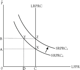
Figure 4.3 Shifts in the short-run labor-force participation rate curve
The unemployment rate is defined as
![]()
where LF is the number of people in the civilian population 16 or older who are either working or looking for work and L the number of people who have work. The labor-force participation rate is
![]()
where POP16 is the size of the civilian population 16 or older.
We can use equations (4.6) and (4.7) to solve for the number of workers:
![]()
It is important not to interpret a fall in the UR, taken alone, to mean that the economy is improving. A fall in the UR causes L to rise, as does a rise in the LFPR, but the same forces that cause the UR to fall can also cause the LFPR to fall. Finally, the result is not just a matter of who is more myopic. Both employed and unemployed workers may leave the labor force as they succumb to the lure of safety-net benefits, as considered in Volume I, Chapter 8.
Misdiagnosing Changes in Real GDP Growth
Just as Y can remain stuck below YFE if the required price and wage adjustments do not take place, ![]() can get stuck below
can get stuck below ![]() normal. Once the economy remains in a prolonged slump, recovery may require government intervention in the form of increased or decreased aggregate demand, whichever corrective is called for. In a Keynesian slump, the appropriate intervention is an increase in aggregate demand relative to supply. In a suppressed-inflation slump, the appropriate intervention is a decrease in aggregate demand relative to supply.
normal. Once the economy remains in a prolonged slump, recovery may require government intervention in the form of increased or decreased aggregate demand, whichever corrective is called for. In a Keynesian slump, the appropriate intervention is an increase in aggregate demand relative to supply. In a suppressed-inflation slump, the appropriate intervention is a decrease in aggregate demand relative to supply.
The question arises, though, just how the government knows what kind of slump the economy is suffering. The question is the length of time over which ![]() is less than
is less than ![]() normal and the amount by which
normal and the amount by which ![]() normal exceeds
normal exceeds ![]() . Some would denote a long-lived excess of
. Some would denote a long-lived excess of ![]() normal over
normal over ![]() as secular stagnation. An unemployment rate persistently greater than the NAIRU is a symptom of a secular stagnation as is a labor-force participation rate persistently less than the NAPR.2 But in any slump, it is likely to be true that both problems will exist—a high unemployment rate and a low labor-force participation rate.
as secular stagnation. An unemployment rate persistently greater than the NAIRU is a symptom of a secular stagnation as is a labor-force participation rate persistently less than the NAPR.2 But in any slump, it is likely to be true that both problems will exist—a high unemployment rate and a low labor-force participation rate.
It is possible to address both problems—high unemployment and low labor-force participation—through policies aimed at removing disincentives to work and/or to create jobs. Such policies shift the LRS curve to the right, increase YFE, increase ![]() normal, reduce the NAIRU, and increase the NAPR.
normal, reduce the NAIRU, and increase the NAPR.
The problem here lies in discerning whether a fall in ![]() is temporary or permanent. Return to the example in which
is temporary or permanent. Return to the example in which ![]() = 5%,
= 5%, ![]() =
= ![]() normal = 3%,
normal = 3%, ![]() = 0 and
= 0 and ![]() Ptargeted = 2%. Now suppose that the actual growth in M temporarily falls from 5% to 4%. Then
Ptargeted = 2%. Now suppose that the actual growth in M temporarily falls from 5% to 4%. Then
![]()
Given the fall in ![]() and assuming that
and assuming that ![]() remains unchanged at zero, both
remains unchanged at zero, both ![]() and
and ![]() must fall by 1 percentage point in order to keep
must fall by 1 percentage point in order to keep ![]() from falling. This is just a dynamic version of the case in which we implicitly assumed that YFE was constant. The only difference is that now it is not a once-and-for-all proportionate fall in W and P that is needed, but a proportionate fall in their growth (again, from 2% to 1%). If this did not occur, then the economy could ratchet itself into a slump, as described here. The policy remedy would be as before—an expansion of government purchases or the money supply to pull the economy back to its normal growth curve.
from falling. This is just a dynamic version of the case in which we implicitly assumed that YFE was constant. The only difference is that now it is not a once-and-for-all proportionate fall in W and P that is needed, but a proportionate fall in their growth (again, from 2% to 1%). If this did not occur, then the economy could ratchet itself into a slump, as described here. The policy remedy would be as before—an expansion of government purchases or the money supply to pull the economy back to its normal growth curve.
We can present a parallel example of “suppressed inflation.” Suppose that the growth in M temporarily rises from 5% to 6%. To close the gap, the growth of P (currently 2%) must rise by 1 percentage point, to 3%. And, likewise, in order to keep the real wage rate from falling, the growth of W (also currently 2%) must rise by 1 percentage point to 3%. Otherwise, employers will put fewer goods on their shelves and workers will withdraw from the labor force.
Casting the discussion in terms of growth rates brings to light the complexities that arise in diagnosing a case of high unemployment or low labor-force participation. First, the growth of the money supply is not tightly controlled from some command post at the Federal Reserve. Controlling the money supply requires answering questions about what definition of the money supply to use, about how tightly the Fed can control the money supply through asset purchases and sales, and about what kind of assets the Fed will choose to buy and sell in conducting its policy. Second, the growth path of YFE changes with innovation booms, Middle East wars, elections, and so forth. Finally, controlling inflation involves the choice of price indexes, distinctions between actual and “core” inflation (goods excluding food and energy), and the need to anticipate and correct for the numerous forces at work in the economy, outside the orbit of monetary and fiscal policy, that cause growth rates to fluctuate unpredictably.
The problem is that it might be hard to tell whether any developing problem of long-term underemployment results from a failure of ![]() and
and ![]() to adjust downward or upward. We cannot assume that there is a failure of these indicators to adjust downward because of an ill-advised decrease in
to adjust downward or upward. We cannot assume that there is a failure of these indicators to adjust downward because of an ill-advised decrease in ![]() . Or that a failure to adjust upward results from an ill-advised increase in
. Or that a failure to adjust upward results from an ill-advised increase in ![]() . Rather, the problem of fine-tuning monetary policy has to do with the behavior of
. Rather, the problem of fine-tuning monetary policy has to do with the behavior of ![]() relative to observed changes in
relative to observed changes in ![]() , which actually means the behavior of k, a point made in Chapter 1 of this volume.
, which actually means the behavior of k, a point made in Chapter 1 of this volume.
Suppose that the monetary authorities are keeping ![]() fixed at 5% and
fixed at 5% and ![]() fixed at 2% but that
fixed at 2% but that ![]() unexpectedly falls from 3% to zero, which leads to, temporarily, at least
unexpectedly falls from 3% to zero, which leads to, temporarily, at least
![]()
Assume that ![]() remains unchanged, which is to say,
remains unchanged, which is to say,
![]()
Now recall that, at the moment before ![]() fell,
fell,
![]()
The question then is whether it continues to be true that
![]()
so that what we see in equation (4.10) is just an anomaly, or whether it is now true that
![]()
Ultimately the economy will adjust in such a way as to satisfy equation (4.3). If policymakers see equation (4.13) as still true, they might interpret the fall in ![]() as having resulted from a temporary rise in the demand for money relative to the supply of money, as manifested by a rise in
as having resulted from a temporary rise in the demand for money relative to the supply of money, as manifested by a rise in ![]() . Were that the case, employers and workers should (i.e., “should” from their own self-interested point of view) agree to bring about proportionate decreases in
. Were that the case, employers and workers should (i.e., “should” from their own self-interested point of view) agree to bring about proportionate decreases in ![]() and
and ![]() . (Note that
. (Note that ![]() is the rate at which people are increasing the fraction of their real income that they want to hold as cash, so that a rise in
is the rate at which people are increasing the fraction of their real income that they want to hold as cash, so that a rise in ![]() brings about a rise in the demand for money relative to the supply and the need for the growth of prices and wages to fall.) If these adjustments do not occur and if
brings about a rise in the demand for money relative to the supply and the need for the growth of prices and wages to fall.) If these adjustments do not occur and if ![]() fails to return to the old normal, then the appropriate policy response, so it would appear, would be to increase
fails to return to the old normal, then the appropriate policy response, so it would appear, would be to increase ![]() until
until ![]() returns to normal, if it ever does.
returns to normal, if it ever does.
Suppose, however, that this is a misdiagnosis, which means for some reason now ![]() normal = 0%, and
normal = 0%, and ![]() did not rise. That means that the growth of the supply of money must ultimately fall relative to the growth of the demand for money. In order to restore equality between the growth of the supply and the growth of the demand for money, the monetary authorities must permit
did not rise. That means that the growth of the supply of money must ultimately fall relative to the growth of the demand for money. In order to restore equality between the growth of the supply and the growth of the demand for money, the monetary authorities must permit ![]() to rise from 2 to 5%, cut
to rise from 2 to 5%, cut ![]() from 5 to 2%, or bring about some combination of the two. Then also, if
from 5 to 2%, or bring about some combination of the two. Then also, if ![]() rises,
rises, ![]() must rise in tandem with
must rise in tandem with ![]() .
.
If ![]() rises and if
rises and if ![]() does not keep pace with
does not keep pace with ![]() , the stage will be set for a suppressed-inflation scenario. The economy can sink into a “supply-side” downturn in which
, the stage will be set for a suppressed-inflation scenario. The economy can sink into a “supply-side” downturn in which ![]() falls below the new (and lower) normal
falls below the new (and lower) normal ![]() . In this case
. In this case ![]() would become negative. Why? Again, because, barring a reduction in monetary growth, nominal wages must rise in proportion to prices in order to keep workers from wanting to cut back on their labor services.
would become negative. Why? Again, because, barring a reduction in monetary growth, nominal wages must rise in proportion to prices in order to keep workers from wanting to cut back on their labor services.
We are back to the situation in which pizza shop managers generally refuse to grant wage increases to their workers, not understanding in this instance, that, despite the shrinkage in business that took place because of the downturn in ![]() normal, the demand for pizza is growing faster than the supply (this is because the growth of M exceeds the growth of Y). While the idea of acceding to wage demands in a slumping economy seems perverse, doing so is in fact necessary here to keep workers on the job, given that workers correctly understand that the underlying upward pressure on
normal, the demand for pizza is growing faster than the supply (this is because the growth of M exceeds the growth of Y). While the idea of acceding to wage demands in a slumping economy seems perverse, doing so is in fact necessary here to keep workers on the job, given that workers correctly understand that the underlying upward pressure on ![]() will otherwise cause their real wages to fall. Now if workers do not get faster raises, they will pull out of their jobs and production will slump even further. The further slump in production will lead workers to pull back still more as the availability of consumer goods (pizzas) further shrinks, and so on. At this point, monetary and fiscal contraction becomes an even more pressing policy imperative.
will otherwise cause their real wages to fall. Now if workers do not get faster raises, they will pull out of their jobs and production will slump even further. The further slump in production will lead workers to pull back still more as the availability of consumer goods (pizzas) further shrinks, and so on. At this point, monetary and fiscal contraction becomes an even more pressing policy imperative.
The trick is to determine whether an observed decline in ![]() is attributable to some shift in preferences such as a rise in
is attributable to some shift in preferences such as a rise in ![]() or whether it is attributable to a decrease in
or whether it is attributable to a decrease in ![]() normal itself. If it is the former and if the decline is long-lasting, then the correct remedy is a governmentally engineered increase in aggregate demand through an increase in
normal itself. If it is the former and if the decline is long-lasting, then the correct remedy is a governmentally engineered increase in aggregate demand through an increase in ![]() . If it is the latter, then it is necessary to see how prices and wages adjust. If
. If it is the latter, then it is necessary to see how prices and wages adjust. If ![]() and
and ![]() rise in tandem, then the economy will slump to its new normal without further, unnecessary decline in output growth. If they do not rise in tandem, then the economy will slump even below its new normal until a government-engineered contraction in aggregate demand is implemented.
rise in tandem, then the economy will slump to its new normal without further, unnecessary decline in output growth. If they do not rise in tandem, then the economy will slump even below its new normal until a government-engineered contraction in aggregate demand is implemented.
What Is the Correct Monetary Rule?
The money supply of the United States fell by 30% during the Great Depression. Real GDP fell by 26% from its peak in 1929 to its trough in 1932. Much of the decline in the money supply was the result of people pulling their money out of banks as they panicked over bank closings. But the Fed arguably allowed the decline in the money supply to take place, with the result that real GDP fell by more than it would have fallen, had the monetary contraction not taken place.
The record of the Fed since the Great Depression has been spotty. Perhaps the period for which the Fed is most highly regarded for its conduct of monetary policy was during the “Great Moderation” of (about) 1985 to 2005, so dubbed by John Taylor because of the simultaneous low inflation, low unemployment, and high GDP growth that characterized that period.
According to the “Taylor rule,” the Federal Reserve should keep the short-term nominal interest rate at a level that satisfies the equation
![]()
where R is the short-term nominal interest rate, Y is actual real GDP, YFE is potential real GDP, ![]() is the actual inflation rate, PTAR is the targeted inflation rate, and r is the natural rate of interest, that is, the rate that equilibrates saving and investment. In an early paper on this topic, Taylor proposed setting g at 0.5, h at 0.5, PTAR at 0.02 and r at 0.02 (Taylor 1998).
is the actual inflation rate, PTAR is the targeted inflation rate, and r is the natural rate of interest, that is, the rate that equilibrates saving and investment. In an early paper on this topic, Taylor proposed setting g at 0.5, h at 0.5, PTAR at 0.02 and r at 0.02 (Taylor 1998).
According to one report, the Taylor rule “correctly predicted the decisions of the Federal Open Market Committee 85 percent of the time up until 2008” (Lowenstein).3 This assessment applies to the actions of the committee during the tenure of Alan Greenspan, who served as chairman of the Federal Reserve Board over most of the Great Moderation. Although the Fed did not formally adopt the Taylor rule as the instrument for guiding monetary policy, it nevertheless gave the rule great importance in making monetary policy decisions.
Taylor himself has stressed the importance of rule-based, as opposed to discretionary, policy making. The Great Moderation, he has argued, testifies to superiority of rules-based monetary policy over “interventionism.” The Taylor rule, as mentioned, became the dominant rule of that period.
However, monetary policy went off the rails in the 2000s.
Between 2003 and 2005, the Federal Reserve held interest rates far below the levels that would have been suggested by monetary policy rules that had guided the Fed’s actions the previous two decades....the Fed’s public statements during that time—which asserted that interest rates would be low for a “prolonged period” and would rise at a “measured pace”—are evidence that this was an intentional departure from the policies of the 1980s and 1990s (Taylor 2013, pp. 34–35).
Taylor testifies to the extraordinary lengths to which the U.S. government went over the course of the following “Great Contraction” to rescue the economy through expansionist monetary and fiscal policies. This was as opposed to his recommended return to the rule-based policy that the Fed had implemented during the previous Great Moderation. According to Taylor, monetary policy was overly expansionist over the entire period 2003 to 2009.
Taylor’s assessment of the conduct of monetary policy during that period is at odds, however, with an alternative line of thinking. To understand this line of thinking, it is necessary to recognize the fact that any Fed policy aimed at controlling interest rates invites the creation of disparities between the Fed-mandated interest rate and the natural interest rate.
The natural interest rate is the r that equilibrates the supply and demand for capital, as derived in Volume I, Chapter 5. In that chapter, we allowed that the nominal interest rate R would diverge from the real rate r as the rate of inflation ![]() rose above or fell below zero. Table 1.1 in Chapter 1 of this volume fleshes out that analysis by tying
rose above or fell below zero. Table 1.1 in Chapter 1 of this volume fleshes out that analysis by tying ![]() to the rate of monetary expansion or contraction. In that chapter, we expanded the analysis to consider how increases or decreases in the money supply can affect real GDP either directly by inducing people to adjust their spending to changes in the money supply or indirectly by influencing nominal interest rates. The Taylor rule calls for a policy of using the Fed’s control over the money supply to fix R at whatever rate achieves the wanted balance between the goal of closing the GDP gap (the gap between actual and full-employment GDP) and the goal of bringing the actual inflation rate into line with the targeted rate.
to the rate of monetary expansion or contraction. In that chapter, we expanded the analysis to consider how increases or decreases in the money supply can affect real GDP either directly by inducing people to adjust their spending to changes in the money supply or indirectly by influencing nominal interest rates. The Taylor rule calls for a policy of using the Fed’s control over the money supply to fix R at whatever rate achieves the wanted balance between the goal of closing the GDP gap (the gap between actual and full-employment GDP) and the goal of bringing the actual inflation rate into line with the targeted rate.
The Taylor rule operates by finding the ideal point on the short-run Phillips curve. An alternative rule would aim strictly at closing the GDP gap. If the Phillips curve is vertical, as it must be in the long run, then the alternative rule would be to adjust the money supply to bring actual GDP into line with potential, full-employment GDP and then, once the GDP gap is closed, to bring the rate of monetary expansion into line with the growth of real GDP and the percentage change in velocity.
In his presidential address to the American Economic Association, Milton Friedman reiterated his long-standing argument that the Fed should adopt a monetary rule—not an interest rate rule. “The first requirement,” he said,
is that the monetary authority should guide itself by magnitudes it can control, not by ones that it cannot control. If, as the authority has often done, it takes interest rates or the current unemployment percentage as the immediate criterion of policy, it will be like a space vehicle that has taken a fix on the wrong star. No matter how sensitive and sophisticated its guiding apparatus, the space vehicle will go astray (Friedman 1968, pp. 14–15).
The correct monetary rule, argued Friedman, would specify “a steady rate of growth in a monetary total.” That would be “something like a 3 to 5 per cent per year rate of growth in currency plus all commercial bank deposits [M1] or a slightly lower rate of growth in currency plus demand deposits only” (Friedman 1968, p. 16).
The average annual growth of M1 over the period 1980 to 2017 was 5.9%. For the same period, ![]() = 2.6% and
= 2.6% and ![]() = −0.8%. Solving for
= −0.8%. Solving for ![]() ,
,
![]()
If 2.6% is the new normal growth rate of real GDP and if 2.5% is the targeted inflation rate, then we can conclude that, going forward, the Fed should adopt the “Friedman rule” and set the annual growth of M1 at 5.9%.
1 Although all the discussion is in terms of monetary policy, every point made in the upcoming text concerning the use of monetary policy can be generalized to encompass fiscal policy as well.
2 Note that the economy can suffer from suppressed inflation even if prices are rising faster than nominal wages. Suppressed inflation exists if prices and wages are not rising as fast as aggregate demand.
3 The Federal Reserve Open Market Committee is the policy arm of the Federal Reserve System, consisting of the seven members of the board of governors plus five presidents of the regional Federal Reserve Banks.