Decision Analysis to Support Ransomware Cybersecurity Risk Management
Robert D. Brown III, Cybersecurity Risk Management Leader, Resilience Insurance
Introduction
With the exception of pure intuitionists, most decision makers understand that making good decisions relies on access to good information in the form of qualified and pedigreed measurements. To this end, Hubbard and Seiersen have accomplished a sizable task by demonstrating that a tractable pathway usually exists to quantify measures that frequently present themselves as very difficult to quantify or that many often assume cannot be quantified at all. This is commendable in itself, but the fact is that measurements, regardless of how important, do little more than to satisfy curiosity unless they support the human effort of making decisions to achieve some goal or objective. Unfortunately, a significant fact will continue to frustrate decision makers supplied with even the best of measurements; that is, few measurements will ever supply such perfect precision about current and future conditions that the best decision pathway forward is clearly unambiguous. Fortunately, with the help of the science of normative decision analysis, we can gain decision clarity with even imperfect and uncertain measurements.
This essay will provide a brief, high‐level overview of the guidance that integrates measurements of the kind Hubbard and Seiersen promote to support cybersecurity decision management activities, especially those for which intended outcomes still face a considerable amount of uncertainty and risk. The example we will consider involves a CISO who wants to understand the decision trade‐offs among the levels of cost of controls that can be implemented to reduce the realization of ransomware threats against the risk‐adjusted and probable range of ransomware impacts if a ransomware event actually occurs. Our example will point out how to make a rational decision that balances the effects of imperfect measurements and low‐probability, high‐impact events.
Framing the Decision
Imagine that you are a new CISO in an organization that has grown rapidly over the last five years. Revenues have risen to $200 million annually. In the rush to grow, however, security wasn't always a high priority. A recent scan of your company's data assets revealed that approximately 30 million records persisted in various states of security hygiene. Given the company's profile in the media, the continued rising tide of ransomware attacks, and the potential points of unmitigated exposure, you are very concerned that your company will face a compromise in security that could cost millions of dollars either through extortion, penalties, and reimbursements for exfiltrated personally identifiable data or business disruption. Furthermore, although you realize that the risk and magnitude of financial loss represents an important metric for the company to consider, the cost is not a dedicated cost as it might not ever materialize. If it does materialize, however, not having implemented reasonable controls to prevent it would be rightly viewed as a dereliction of duty as an information security officer. At times the market for security controls looks like a carnival for wares of varying quality. Knowing what to buy presents a difficult enough problem, but since many of the best‐known solutions don't come cheaply, justifying an actual dedicated budget for them to the CFO is fraught with even more difficulties. Certainly, the effort to reduce the threat deserves some allocation of resources, but it does not warrant the employment of all available resources to that end. The primary question to address is: what level of security controls, given their associated cost to implement, minimizes the economic value at risk to the organization to reduce the potential impact of ransomware attack?
Before you get started crunching numbers, you will want to map out an abstraction of the problem in the form of an influence diagram, as illustrated in Figure B.1. The diagram illustrates the essence of the problem to other key collaborators and stakeholders in terms of the uncertainties you face, decisions to be made, and their effect on the value at risk to the organization. As a result, you will have a registry of key uncertainties that put you at risk and a framework for building the financial analysis that will support making a final decision.
The influence diagram reflects that decision strategies are composed of combinations of security control levels as displayed in the table of Figure B.2.
Suppose that Decision1 is a base case reflecting the current condition that all controls are in an unmanaged state. Decision2 might be the most aggressive case with all of the controls set to their highest level. Decisions 1 and 2 are decision strategies. You believe the combination of controls bears a relationship to the arrival rate of experiencing a material, reportable events in any year such that the higher the level of control, the lower that rate is. However, the cost of the chosen controls is also relevant to the decision strategy, but in this case the higher the level of control, the higher the cost. Finally, you reflect your beliefs about the key loss impacts:

FIGURE B.1 Influence diagram of ransomware model
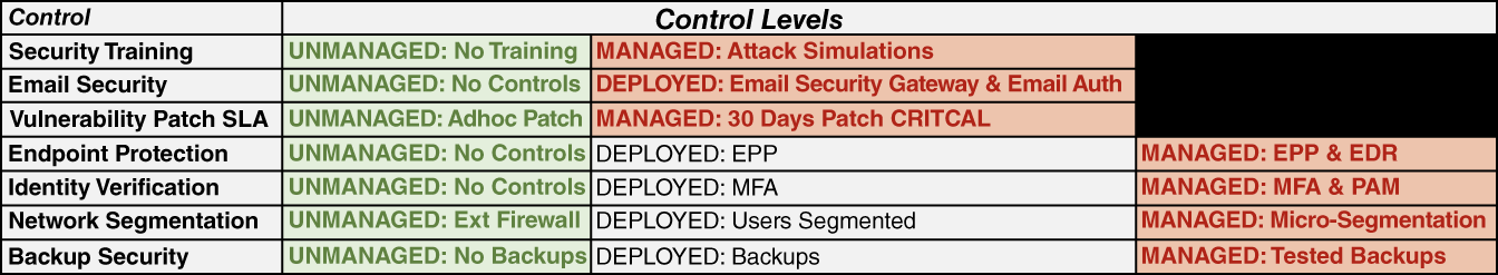
FIGURE B.2 Control level configurations for Decision1 and Decision2
- The level of extortion demanded by a threat actor is proportional to your revenues, but the final payout would be negotiable (the bad guys are in business, too!).
- The impact of business disruption would be dependent on the duration of the disruption and the unit daily cost of being down.
- The effect of data exfiltration will be directly proportional to the number of records at risk and a unit record cost.
What You Will Need
While this discussion relies on the use of the R programming language, you will be able to read along and understand the essential concepts without knowing anything about either programming or programming in R specifically. However, if you decide to implement the code to study it for yourself to understand the underlying concepts, you will need to install The R Programming Language for Statistical Computing, a good integrated development environment (IDE) such as RStudio, and the packages tidyverse, reshape2, and scales. Most of the code will rely on base R to help you focus more on the essential concepts rather than idiosyncrasies of specific packages. The full source code demonstrated here is available at the book website www.themetricsmanifesto.com.
Setting Up the Analysis
We base the following set of assessments on the assumption that you have done your homework according to the guidance in this book to achieve reasonable measurements. (Note, though, that the values are chosen to illustrate the modeling process and insights derived from it. They do not necessarily reflect the results of actual research.)
- 4.1. Arrival Rates of a Material Event: You assess the average time between material, reportable events to be seven years under the Decision1 level of controls and 35 years under Decision2. You model this as an Exponential(1/t) distribution, where t is the average number of years. However, you strongly suspect that the time between events won't be less than 1/3 of the average you calculated from just a few data points.
- 4.2. Costs of Controls: After conferring with several vendors and other CISOs, you assess the range of annual costs associated with the Decision2 control levels. You model these as Triangular(lb, mode, ub) for each year of your model.
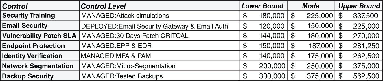
FIGURE B.3 Cost of controls for Decision2
- 4.3. Distributions of Impact
- 4.3.1. Extortion Revenue Factor [% revenue] = Normal(mean = 0.035, sd = 0.013)
- 4.3.2. Extortion Settlement Fraction [% demand] = Normal(mean = 0.5, sd = 0.084)
- 4.3.3. Business Disruption Duration [days] = Lognormal(meanlog = log(4.5), sdlog = 0.7)
- 4.3.4. Records at Risk = min(10e9, Lognormal(meanlog = ln(30e6), sdlog = 0.5))
- 4.3.5. Data Exfiltration Impact Factor [$/record] = exp(−0.58 ln(R) + 8.2 + Normal(mean = 0, sd =1.6)), where R is records at risk.1
The Decision Model Function
The source code used to support this discussion is in the R script file “HTMA DA Chapter.R” and can be downloaded at www.themetricsmanifesto.com. The pseudocode snippet for the model function takes the following form:
Calc_Ransomware_Model <- function() {exfiltration impact = impact factor * records at risk * events per yearextortion impact = revenue factor * annual revenue * settlement fraction * events per yearbusiness disruption = min(disruption duration * events per year, operating days) * daily revenueannual security costs = total annual cost of controls applied to each year}
Business Model Insights
When we run the model simulation and query it for results based on the assessments and business logic, we see that Decision1 presents a 46% chance of seeing one or more events over the next three years, but Decision2 reduces to 13%. That's approximately equivalent to calling the outcome against a die with two sides to one with eight.
The 90th percentile range of the total security cost (Figure 4: Total Security Cost) over the three years will fall between ~$4.7M and ~$5.6M with an average cost of ~$5.1M (solid vertical line). It's important to observe that if you merely use the sum of the annual cost modes as a best guess (~$4.6M, the dotted vertical line) for your budget, you will face ~97% chance of a budget overrun.
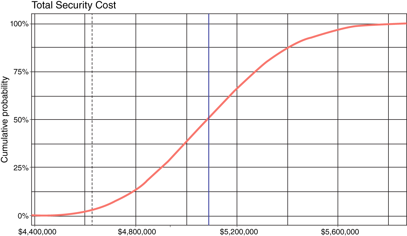
FIGURE B.4 Total Security Cost of controls for Decision2
What happens on the bad days? The following loss exceedance chart (Figure 5: Total Loss Impact) tells you the probability of facing loss impacts greater than some amount. Given your analysis, you observe ~1% chance of exceeding $168M and $70M for Decision1 and Decision2, respectively. The average loss impact for Decision1 occurs at ~$30M (dotted vertical red line) and Decision2 at ~$6M (solid vertical green line), buying an average benefit of ~$24M in avoided loss at a 370% return on cost of controls.
If you net the difference between the Total Security Cost distribution and the Total Loss Impact distributions, you score an average net total cost benefit of ~$19M (Figure 6: Net Total Cost chart, vertical red line), although you still face a 58% probability of increasing your costs overall. This is because control costs are dedicated but avoided loss impacts are only potentially realized, and when they are realized the total cost might be lower than in the choice of doing nothing. As managers of risk, we need to bet against the possible future, and our decision‐making must price in those potential losses.

FIGURE B.5 The loss exceedance curve for Total Loss Impact for each decision

FIGURE B.6 The Net Total Cost for each decision. Positive values indicate a cost benefit of Decision2 over Decision1
Before evaluating the Net Total Cost, you find that the average Total Cost for each decision is ~$30M and ~$11M for Decision1 and Decision2, respectively. If all you cared about was the average, then based on this difference you should be inclined to accept Decision2 as the rational path forward. However, you might ask if any of the uncertainties would make you regret this choice; that is, would any of the uncertainties cause you to prefer Decision1 over Decision2 if they realized either extreme of their imputed ranges?
The tornado chart below (Figure 7) displays which uncertainties expose you to the most potential range of average Total Cost by decision strategy. In this chart, each bar shows how sensitive the average Total Costs are to 80th percentile swings in the uncertainties. If the bars of a particular uncertainty overlap, you might take the opportunity to buy more information about the uncertainty to reduce the ambiguity about which decision is the best decision, or you might buy more control over the uncertainty. In this case, the only two uncertainties that might be candidates for such further analysis or strategic refinement are “time_between_events” and “records_at_risk” (which does not show overlap, but it might be close enough for concern). However, since “records_at_risk” is independent of the decision strategies, the value of information on it would be $0. The “time_between_events” can cause you regret, and a rough value of perfect information calculation2 shows that ~$1.2M should be the most that you should dedicate to gaining enough information about this uncertainty to make an unambiguous decision.
Lastly, you should observe that no single control cost imposes enough uncertainty to make you reconsider your decision to take Decision2. The combination of their effects reduces the arrival rate of the material events enough to justify their spend.

FIGURE B.7 The Total Cost Sensitivity for each decision. The bars associated with each decision reflect how much the average cost of a decision can change due to the effect of the associated named uncertainty. Bars that overlap represent “critical uncertainties” worthy of refined analysis
Questions for Further Consideration
Of course, this is a highly simplified model that could be extended into other dimensions of consideration and nuance. The immediate point is that important independent measurements can be integrated into a decision model that guides organizational leaders who need to measure the monetary value of cybersecurity and gain insights into the best way to allocate resources to achieve it compared to other efficient uses of the resources. Still, other questions remain that decision modeling can address, for example:
- What is the value of third‐party insurance versus self‐insuring?
- How much retention (i.e., deductible) would you be willing to bear before insurance benefits cover realized losses?
- What premium would you be willing to pay?
- How should you cover the tail risk that exceeds the loss limits of an insurance policy?
- Are there other financially feasible control combinations that achieve similar levels of risk reduction without imposing an unacceptable degree of moral hazard?
Notes
- 1 This is based on a linear regression of log‐log cost‐to‐records chart in the 2015 Verizon DBIR report.
- 2 The details of value of information calculations are beyond the scope of this chapter. Roughly described, however, it is the difference between the expected value of knowing the best outcome before making a decision and the decision that maximizes expected value before knowing the best outcome. For more details, see chapter 13: “Setting a Budget for Making Decisions Clearly,” in Business Case Analysis with R: Simulation Tutorials to Support Complex Business Decisions. (https://link.springer.com/book/10.1007/978-1-4842-3495-2).