13

Multiple Regression

Overview

This chapter shows how to perform multiple regression analysis to investigate the relationship between a continuous response variable and multiple continuous predictor variables. It describes the different components of the multiple regression equation, discusses the meaning of R2 and other results from a multiple regression analysis. It shows how bivariate correlations, multiple regression coefficients, and uniqueness indices can be reviewed to assess the relative importance of predictor variables. Fictitious data are examined using the Multivariate platform and the Fit Model platform in JMP to show how the analysis can be conducted and to illustrate how the results can be summarized in tables and in text.

Overview

Introduction to Multiple Regression

Multiple Regression and ANOVA

Multiple Regression and Naturally Occurring Variables

How Large Must My Sample Be?

Cause and Effect Relationships

Predicting a Response from Multiple Predictors

A Simple Predictive Equation

An Equation with Weighted Predictors

Regression Coefficients and Intercepts

The Principle of Least Squares

The Results of a Multiple Regression Analysis

The Multiple Correlation Coefficient

Variance Accounted for by Predictor Variables

Variance Accounted for by Correlated Predictor Variables

Multiple Regression Coefficients

Example: A Test of the Investment Model

Overview of the Analysis

Gathering Data

The JMP Data Table

Computing Simple Statistics and Correlations

Univariate Statistics

Bivariate Correlations

Review Simple Statistics and Correlation Results

Interpret the Correlations

Estimating the Full Multiple Regression Equation

Using the Fit Model Platform

Review the Multiple Regression Results

Uniqueness Indices for the Predictors

Summarizing the Results

Correlation Results from the Multivariate Platform

Regression Results from the Fit Model Platform

Getting the Big Picture

Formal Description of Results for a Paper

Summary

Appendix: Assumptions Underlying Multiple Regression

References

Introduction to Multiple Regression

Multiple regression is a highly flexible procedure that enables researchers to address many different types of research questions. One of the most common multiple regression analyses involves a single numeric continuous response variable and multiple numeric continuous predictors.

For example, suppose you want to find the relative importance of variables believed to predict income. To conduct your research, you obtain information for 1,000 adults. The response variable in your study is annual income for these participants. The predictor variables are current age, years of education, and years in workforce. In this study, the response variable and the predictor variables are all numeric continuous scales. Therefore, multiple regression is the appropriate data analysis procedure.

Analysis with multiple regression addresses a number of research questions. For example, it allows you to determine

• whether there is a significant relationship between the response variable and the multiple predictor variables examined as a group
• whether the multiple regression coefficient for a given predictor variable is statistically significant. This coefficient represents the amount of weight given to a specific predictor, while holding constant the other predictors
• whether a given predictor accounts for a significant amount of variance in the response, beyond the variance accounted for by the other predictors

A multiple regression analysis tells you about the relative importance of the predictor variables included in the multiple regression equation. Researchers conducting nonexperimental research in the social sciences are often interested in learning about the relative importance of naturally occurring predictor variables such as age and income. This chapter shows how to perform such analyses.

There are many other types of regression analyses that are beyond the scope of this book. In the study dealing with annual income, all predictor variables are numeric continuous variables and there is a linear relationship between the predictor variables and the response. This chapter provides an introduction to multiple regression, but it does not cover circumstances that use nominal predictor variables or test nonlinear relationships. Once you learn the basics of multiple regression, you can learn more about advanced regression topics in Cohen, Cohen, West, and Aiken (2003), or Pedhazur (1982).

Multiple Regression and ANOVA

Chapters 8 through 12 presented analysis of variance (ANOVA) procedures, which are commonly used to analyze data from experimental research, in which one or more categorical independent predictor variables (experimental conditions) are manipulated to determine how they affect the study’s dependent variable.

For example, imagine you are interested in studying prosocial behavior—actions intended to help others. Examples of prosocial acts might include donating money to the poor, donating blood, doing volunteer work at a hospital, and so forth. Suppose you develop an experimental treatment (such as promise of reward) that you believe increases the likelihood that people will engage in prosocial acts. To investigate this treatment, you conduct an experiment in which you manipulate the independent variable (half of your participants are given the experimental treatment and half are given a placebo treatment). You then assess the dependent variable, which is the number of prosocial acts that the participants later perform. It would be appropriate to analyze data from this study using one-way ANOVA because there is a single numeric response (number of prosocial acts) and a single nominal predictor variable (experimental group—reward or no reward).

Multiple regression is similar to ANOVA in at least one important respect—both analyses require a numeric continuous response variable. Recall from Chapter 1 that a continuous variable can assume a large number of values. The number of prosocial acts performed over a six-month period can be considered a continuous variable because subjects demonstrate a wide variety of scores, such as 0, 4, 10, 11, 20, 25, 30, and so forth.

However, multiple regression also differs from ANOVA. When data are analyzed with ANOVA, the predictor variable is a categorical variable whose values indicate group membership. In contrast, the predictor variables in multiple regression are usually numeric continuous variables.

As an illustration, assume that you conduct a study in which you administer a questionnaire to a group of participants to assess the number of prosocial acts each has performed. You then go on to obtain scores for the same participants on each of the following predictor variables:

• age
• income
• a questionnaire-type scale that assesses level of moral development.

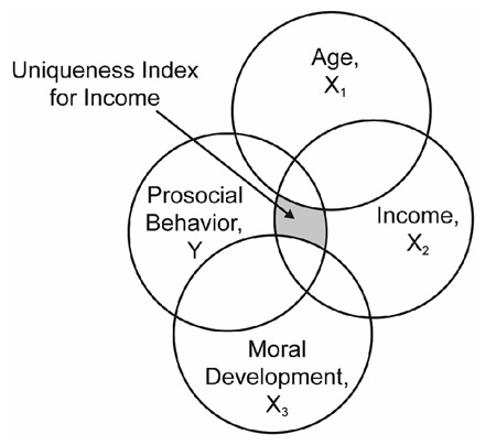
Suppose you have a hypothesis that the number of prosocial acts performed is causally determined by these three predictor variables, as illustrated by the model in Figure 13.1.

Figure 13.1: A Model of Determinants of Prosocial Behavior

The predictor variables in this study (Age, Income, and Moral Development) are continuous. Continuous predictor variables and a continuous response variable means you can analyze your data using multiple regression.

That is the most important distinction between the two statistical procedures. With ANOVA, the predictor variables are always categorical, but with multiple regression, predictor variables are usually continuous. For more information, see Cohen, Cohen, West, and Aiken (2003), or Pedhazur (1982).

Multiple Regression and Naturally Occurring Variables

Multiple regression is particularly well-suited for studying the relationship between naturally occurring predictor and response variables. The researcher does not manipulate naturally occurring variables—they are simply measured as they naturally occur. The preceding prosocial behavior study provides a good example of the naturally occurring predictor variables age, income, and level of moral development.

Research in the social sciences often focuses on naturally occurring variables, which makes multiple regression an important tool. Those kinds of variables cannot be experimentally manipulated. As another example, suppose you have a hypothesis that domestic violence (an act of aggression against a domestic partner) is caused by

• childhood trauma experienced by the abuser
• substance abuse
• low self-esteem

Figure 13.2 illustrates the model for this hypothesis. In this example you cannot experimentally manipulate the predictor variables of the model and later observe the participants as adults to see if the manipulation affected their propensity for domestic violence. However, it is possible to measure these variables as they naturally occur and determine whether they are related to one another in the predicted fashion. Multiple regression allows you to do this.

Figure 13.2: A Model of the Determinants of Domestic Violence

This does not mean that ANOVA is only for the analysis of manipulated predictor variables and multiple regression is only for the analysis of naturally occurring variables. Naturally occurring variables can be predictor variables in an ANOVA provided they are categorical. For example, ANOVA can be used to determine whether participant gender (a naturally occurring predictor variable) is related to relationship commitment (a response variable). In addition, JMP can analyze a categorical manipulated variable, such as an experimental condition, as a predictor variable in multiple regression, but the examples in this chapter cover only numeric continuous predictors. The main distinction to remember is

• ANOVA predictor variables must be categorical variables
• multiple regression predictor variables can be categorical but are usually continuous

Note: An analysis that has both categorical and numeric continuous predictor variables is often referred to as analysis of covariance (ANCOVA). In this kind of model, the continuous predictor variable is called a covariate.

How Large Must My Sample Be?

Multiple regression is a large-sample procedure. Unreliable results might be obtained if the sample does not include at least 100 observations and preferably 200 observations. The greater the number of predictor variables included in the multiple regression equation, the greater the number of participants that will be necessary to obtain reliable results. Most experts recommend at least 15 to 30 participants per predictor variable. See Cohen (1992).

Cause and Effect Relationships

Multiple regression can determine whether a given set of variables is useful for predicting a response variable. Among other things, this means that multiple regression can be used to determine

• whether the relationship between the response variable and predictor variables (taken as a group) is statistically significant
• how much variance in the response is accounted for by the predictor variables
• which predictor variables are relatively important predictors of the response

Although the preceding section often refers to causal models, it is important to remember that the procedures discussed in this chapter do not provide strong evidence concerning cause-and-effect relationships between predictor variables and the response. For example, consider the causal model for predicting domestic violence presented in Figure 13.2. Assume that naturally occurring data for these four variables are gathered and analyzed using multiple regression. Assume further that the results are significant—that multiple regression coefficients for all three of the predictor variables are significant and in the predicted direction. Even though these findings are consistent with your theoretical model, they do not prove that these predictor variables have a causal effect on domestic violence. Because the predictor variables are probably correlated, there can be more than one way to interpret the observed relationships between them. The most that you can say is that your findings are consistent with the causal model portrayed in Figure 13.2. It is incorrect to say that the results prove that the model is correct.

There are a number of reasons to analyze correlational data with multiple regression. Often, researchers are not really interested in testing a causal model. The purpose of the study could simply be to understand relationships between a set of variables.

However, even when the research is based on a causal model, multiple regression can still give valuable information. For example, suppose you obtain correlational data relevant to the domestic violence model of Figure 13.2, and none of the regression coefficients are significant. This is useful because it shows that the model failed to survive an analysis that investigated the predictive relationships between the variables.

However, if significant results are obtained, you can prepare a research report stating that the results were consistent with the hypothesized model. In other words, the model survived an attempt at disconfirmation. If the predictor variables can be ethically manipulated, you could conduct a follow-up experiment to determine whether the predictors appear to have a causal effect on the response variable under controlled circumstances.

In summary, it is important to remember that the multiple regression procedures discussed in this chapter do not provide evidence of cause and effect relationships. However, they are extremely useful for determining whether one set of variables can predict variation in a response.

Note: Use of the term prediction in multiple regression should not be confused with causation.

Predicting a Response from Multiple Predictors

The response variable (also called a predicted or dependent variable) in multiple regression is represented with the symbol Y, and is therefore often referred to as the Y-variable. The predictor variables (also known as independent variables or factors) are represented as X1, X2, X3… Xn, and are referred to as the X-variables. The purpose of multiple regression is to understand the relationship between the Y-variable and the X-variables when taken as a group.

A Simple Predictive Equation

Consider the model of prosocial behavior shown previously in Figure 13.1. The model hypothesizes that the number of prosocial acts performed by a person in a given period of time can be predicted by the participant’s age, income, and level of moral development.

Notice that each arrow (assumed predictive path) in the figure is identified with either a plus (+) sign or a minus (–) sign. A plus sign indicates that you expect the relevant predictor variable to demonstrate a positive relationship with the response, whereas a minus sign indicates that you expect the predictor to demonstrate a negative relationship with the response.

The nature of these signs in Figure 13.1 shows that you expect

• a positive relationship between age and prosocial behavior, meaning that older participants tend to perform more prosocial acts
• a positive relationship between income and prosocial behavior, meaning that more affluent people tend to perform more prosocial acts
• a positive relationship between moral development and prosocial behavior, meaning that participants who score higher on the paper-and-pencil measure of moral development tend to perform more prosocial acts

Assume that you administer a questionnaire to a sample of 100 participants to assess their level of moral development. Scores on this scale can range from 10 to 100, with higher scores reflecting higher levels of moral development. From the same participants, you also obtain age and information about their income. You now want to use this information to predict the number of prosocial acts the participant will perform in the next six months. More specifically, you want to create a new variable, , that represents your best guess of how many prosocial acts the participants will perform. Keep in mind that represents the prediction of the participants’ standing on the response variable. Y is the participants’ actual standing on the response variable.

Assume the predictor variables are positively related to prosocial behavior. One way to predict how many prosocial behaviors in which participants will engage could be to simply add together the participants’ scores on the three X variables. This sum, as expressed by the following equation, then constitutes your best guess as how many prosocial acts they will perform.

= X1 + X2 + X3

where

= the participants’ predicted scores on prosocial behavior

X1 = the participants’ actual scores on age

X2= the participants’ actual scores on income (in thousands)

X3 = the participants’ actual scores on the moral development scale

To make this more concrete, consider the fictitious data presented in Table 13.1. This table presents actual scores for four of the study’s participants on the predictor variables.

Table 13.1: Fictitious Data, Prosocial Behavior Study

Participant	Age X1	Income (In Thousands) X2	Moral Development X3
Lars	19	15	12
Sally	24	32	28
Jim	33	45	50
. . .	. . .	. . .	. . .
Sheila	55	60	95

To arrive at an estimate of the number of prosocial behaviors predicted for the first participant (Lars), insert his scores on the three X variables into the preceding equation:

= X1 + X2 + X3

= 19 + 15 + 12

= 46

So your best guess is that the first participant, Lars, will perform 46 prosocial acts in the next six months. You can repeat this process for all participants and compute their scores in the same way. Table 13.2 presents the predicted scores on the prosocial behavior variable for some of the study’s participants.

Notice the general relationships between and the X variables in Table 13.2. If participants have low scores on age, income, and moral development, your equation predicts that they will engage in relatively few prosocial behaviors. However, if participants have high scores on these X variables, then your equation predicts that they will engage in a relatively large number of prosocial behaviors. For example, Lars had relatively low scores on these X variables, and as a consequence, the equation predicts that he will perform only 46 prosocial acts over the next six months. In contrast, Sheila displayed higher scores on age, income, and moral development, so your equation predicts that she will engage in 210 prosocial acts.

Table 13.2: Predicted Scores for Fictitious Data, Prosocial Behavior Study

Participant	Predicted Scores on Prosocial Behavior	Age X1	Income (In Thousands) X2	Moral Development X3
Lars	46	19	15	12
Sally	84	24	32	28
Jim	128	33	45	50
. . .		. . .	. . .	. . .
Sheila	210	55	60	95

You have created a new variable,. Imagine that you now gather data regarding the actual number of prosocial acts these participants engage in over the following six months. This variable is represented with the symbol Y because it represents the participants’ actual scores on the response and not their predicted scores. You can list these actual scores in a table with their predicted scores on prosocial behavior, as shown in Table 13.3.

Notice that, in some cases, the participants’ predicted scores on Y are not close to the actual scores. For example, your equation predicted that Lars would engage in 46 prosocial activities, but in reality he engaged in only 10. Similarly, it predicted that Sheila would engage in 210 prosocial behaviors, while she actually engaged in only 130.

Despite these discrepancies, you should not lose sight of the fact that the new variable does appear to be correlated with the actual scores on Y. Notice that participants with low scores (such as Lars) also tend to have low scores on Y, and participants with high scores (such as Sheila) also tend to have high scores on Y. There is probably a moderately high product-moment correlation (r) between Y and . This correlation supports your model as it suggests that there really is a relationship between Y and the three X variables when taken as a group.

Table 13.3: Actual and Predicted Scores for Fictitious Data, Prosocial Behavior Study

Participant	Actual Scores on Prosocial Behavior Y	Predicted Scores on Prosocial Behavior
Lars	10	46
Sally	40	84
Jim	70	128
. . .	. . .	. . .
Sheila	130	210

The procedures (and the predictive equation) described in this section are for illustration only. They do not describe the way that multiple regression is actually performed. However, they do illustrate some important basic concepts in multiple regression analysis. In multiple regression analysis,

• You create an artificial variable, , to represent your best guess of the participant’s standings on the response variable.
• The relationship between this variable and the participant’s actual standing on the response (Y) is assessed to indicate the strength of the relationship between Y and the X variables when taken as a group.

Multiple regression has many important advantages over the practice of simply adding together the X variables as illustrated in this section. With true multiple regression, the various X variables are multiplied by optimal weights before they are added together to create . This usually results in a more accurate estimate of the participants’ standing on the response variable. In addition, you can use the results of a true multiple regression procedure to determine which of the X variables are more important predictors of Y, and which variables are less important predictors of Y.

An Equation with Weighted Predictors

In the preceding section, each predictor variable has an equal weight (1) when computing scores on . You did not, for example, give twice as much weight to income as you gave to age when computing scores. Assigning equal weights to the various predictors makes sense in some situations, especially when all of the predictors are equally predictive of the response.

However, what if your measure of moral development displayed a strong correlation with prosocial behavior (r = 0.70, for example), income demonstrated a moderate correlation with prosocial behavior (r = 0.40), and age demonstrated only a weak correlation with prosocial behavior (r = 0.20)? In this situation, it would make sense to assign different weights to the different predictors. For example, you might assign a weight of 1 to age, a weight of 2 to income, and a weight of 3 to moral development.

The predictive equation that reflects this weighting scheme is

= (1)X1 + (2)X2 + (3)X3

where X1 = age, X2 = income, and X3 = moral development. To calculate a given participant’s score for , multiply the participant’s score on each X variable by the appropriate weight and sum the resulting products. For example, Table 13.2 showed that Lars had a score of 19 on X1, a score of 15 on X2, and a score of 12 on X3.

Using weights, his predicted prosocial behavior score, , is calculated as

= (1)X1 + (2)X2 + (3)X3

= (1)19 + (2)15 + (3)12

= 85

This weighted equation predicts that Lars will engage in 85 prosocial acts over the next six months. You could use the same weights to compute the remaining participants’ scores for . Although this example has again been somewhat crude in nature, it is the concept of optimal weighting that is at the heart of multiple regression analysis.

Regression Coefficients and Intercepts

In linear multiple regression as performed by the Fit Model platform in JMP, optimal weights are automatically calculated by analysis.

The following symbols are used to represent the various components of an actual multiple regression equation

= b1X1 + b2X2 + b3X3 ... bnXn + a

where

= the participants’ predicted scores on the response variable

bk = the nonstandardized multiple regression coefficient for the kth predictor variable

Xk = kth predictor variable

a = the intercept constant

A multiple regression coefficient for a given X variable represents the average change in Y associated with a one-unit change in that X variable, while holding constant the remaining X variables.

This somewhat technical definition for a regression coefficient is explained in more detail in a later section. For the moment, it is useful to think of a regression coefficient as revealing the amount of weight that the X variable is given when computing . In this book, nonstandardized multiple regression coefficient are referred to as b weights.

The symbol a represents the intercept constant of the equation. The intercept is a fixed value added to or subtracted from the weighted sum of X scores when computing .

To develop a true multiple regression equation using the Fit Model platform in JMP, it is necessary to gather data on both the Y variable and the X variables. Assume that you do this in a sample of 100 participants. You analyze the data, and the results of the analyses show that the relationship between prosocial behavior and the predictor variables can be described by the following equation:

= b1X1 + b2X2 + b3X3 + a

= (0.10)X1 + (0.25)X2 + (1.10)X3 + (–3.25)

The preceding equation indicates that your best guess of a given participant’s score on prosocial behavior can be computed by multiplying the age score by 0.10, multiplying the income score by 0.25, and multiplying the moral development score by 1.10. Then, sum these products and subtract the intercept of 3.25 from this sum.

This process is illustrated by inserting Lars’ scores on the X variables in the following equation:

= (0.10)19 + (0.25)15 + (1.10)12 + (–3.25)

= 1.9 + 3.75 + 13.2 + (–3.25)

= 18.85 + (–3.25)

= 15.60

Your best guess is that Lars will perform 15.60 prosocial acts over the next six months. You can calculate the scores for the remaining participants in Table 13.2 by inserting their X scores in this same equation.

The Principle of Least Squares

At this point it is reasonable to ask, “How did the analysis program determine that the optimal b weight for X1 was 0.10? How did it determine that the optimal weight for X2 was 0.25? How did it determine that the ‘optimal’ intercept (a term) was –3.25?”

The answer is that these values are optimal in the sense that they minimize a function of the errors of prediction. An error of prediction refers to the difference between a participant’s actual score on the response (Y) and predicted score on the response (). This difference can be written

Y –

Remember that you must gather actual scores on Y in order to perform the multiple regression analysis that computes the error of prediction (the difference between Y and ) for each participant in the sample. For example, Table 13.4 reports several participants’ actual scores for Y and their predicted scores for Y based on the optimally weighted regression equation above, and their errors of prediction.

Table 13.4: Prediction Errors Using Optimally Weighted Multiple Regression Equation

Participant	Actual Scores on Prosocial Behavior Y	Predicted Scores on Prosocial Behavior	Errors of Prediction Y –
Lars	10	15.6	–5.60
Sally	40	37.95	2.05
Jim	70	66.30	3.70
. . .	. . .	. . .	. . .
Sheila	130	121.75	8.25

For Lars, the actual number of prosocial acts performed was 10, while the multiple regression equation predicted that he would perform 15.60 acts. The error of prediction for Lars is 10 – 15.60 = –5.60. The errors of prediction for the remaining participants are calculated in the same fashion.

Earlier it was stated that the b weights and intercept calculated by regression analysis are optimal in the sense that they minimize errors of prediction. More specifically, these weights and intercept are computed according to the principle of least squares. The principle of least squares says that values are calculated such that the sum of the squared errors of prediction is a minimal.

This principal of least squares means that no other set of b weights and intercept constant gives a smaller value for the sum of the squared errors of prediction.

The sum of the squared errors of prediction is written

∑(Y – )2

To compute the sum of the squared errors of prediction according to this formula, it is necessary to

1. compute the error of prediction (Y – ) for a given participant

2. square this error

3. repeat this process for all remaining participants

4. sum the resulting squares. The purpose of squaring the errors before summing them is to eliminate the negative error values that cause the sum of errors to be zero.

When analyzing a JMP data table using multiple regression, the Fit Model platform applies a set of formulas that calculates the optimal b weights and the optimal intercept for that data. These calculations minimize the squared errors of prediction. That is, regression calculates optimal weights and intercepts. They are optimal in the sense that no other set of b weights or intercepts could do a better job of minimizing squared errors of prediction for the current set of data.

With these points established, it is finally possible to summarize what multiple regression actually lets you to do.

Multiple regression lets you to examine the relationship between a single response variable and an optimally weighted linear combination of predictor variables.

In the preceding statement,

• is the optimally weighted linear combination of predictor variables.
• Linear combination means the various X variables are combined or added together to arrive at.
• Optimally weighted means that X variables have weights that satisfy the principle of least squares.

Although we think of multiple regression as a procedure that examines the relationship between single response variables and multiple predictor variables, it is also a procedure that examines the relationship between just two variables, Y and .

The Results of a Multiple Regression Analysis

The next sections describe important information given by the multiple regression analysis. Details include how to compute and interpret

• the multiple correlation coefficient
• the amount of variation accounted for by predictor variables
• the effect of correlated predictor variables

The Multiple Correlation Coefficient

The multiple correlation coefficient, symbolized as R, represents the strength of the relationship between a response variable and an optimally weighted linear combination of predictor variables. Its values range from 0 through 1. It is interpreted like a Pearson product-moment correlation coefficient (r) except that R can only assume positive values. Values approaching zero indicate little relationship between the response and the predictors, whereas values near 1 indicate strong relationships. An R value of 1.00 indicates perfect or complete prediction of response values.

Conceptually, R is the product-moment correlation between Y and. This can be symbolized as

R = rYY'

In other words, if you obtain data from a sample of participants that includes their scores on Y and a number of X variables, compute scores for each participant and then find the correlation of predicted response scores () with actual scores (Y). That bivariate correlation coefficient is R, which is the multiple correlation coefficient.

With bivariate regression, the square of the correlation coefficient between Y and X estimates the proportion of variance in Y accounted for by X. The result is sometimes called the coefficient of determination. For example, if r = 0.50 for a given pair of variables, then

coefficient of determination = r2

= (0.50)2

= 0.25

You can say that the X variable accounts for 25% of the variance in the Y variable.

An analogous coefficient of determination can be computed in multiple regression by squaring the observed multiple correlation coefficient, R. This R2 value (often referred to as R-squared) represents the percentage of variance in Y accounted for by the linear combination of predictor variables given by the multiple regression equation. The next section gives details about the concept of variance accounted for.

Variance Accounted for by Predictor Variables

In multiple regression analyses, researchers often speak of variance accounted for, which is the percent of variance in the response variable accounted for by the linear combination of predictor variables.

A Single Predictor Variable

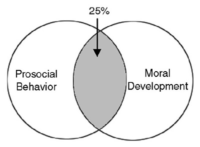
This concept is easy to understand with a simple bivariate example. Assume that you compute the correlation between prosocial behavior and moral development and find that r = 0.50. You can determine the percentage of variance in prosocial behavior accounted for by moral development by squaring this correlation coefficient:

R2 = (0.50)2 = 0.25

Thus, variation in moral development accounts for 25% of the variance in the prosocial behavior response data. This can be graphically illustrated with a Venn diagram that uses circles to represent total variance in a variable. Figure is a Venn diagram that represents the correlation between prosocial behavior and moral development.

The circle for moral development overlaps the circle for prosocial behavior, which indicates that the two variables are correlated. More specifically, the circle for moral development overlaps about 25% of the circle for prosocial behavior. This illustrates that moral development accounts for 25% of the variance in prosocial behavior.

Figure 13.3: Variance in Prosocial Behavior Accounted for by Moral Development

Multiple Predictor Variables with Correlations of Zero

The idea of variance accounted for can be expanded to the situation in which there are multiple X variables. Assume that you obtain data on prosocial behavior, age, income, and moral development from a sample of 100 participants and compute correlations between the four variables as summarized in Table 13.5.

Table 13.5: Correlation Matrix: Zero Correlations between X Variables

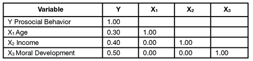
The correlations for a set of variables are often presented in the form of a correlation matrix such as the one presented in Table 13.5. The intersection of the row for one variable and the column for another variable identifies the correlation between the two variables. For example, where the row for X1 (age) intersects with the column for Y (prosocial behavior), you see the correlation (r) between age and prosocial behavior is 0.30.

You can use these correlations to determine how much variance in Y is accounted for by the three X variables. For example, the correlation, r, between age and prosocial behavior is 0.30; therefore, R2 is 0.09 (0.30 x 0.30 = 0.09). This means that age accounts for 9% of the variance in prosocial behavior. Following the same procedure, you learn that income accounts for 16% of the variance in Y (0.40 x 0.40 = 0.16), and moral development continues to account for 25% of the variance in Y.

Notice in Table 13.5 that each of the X variables demonstrates a correlation of zero with all of the other X variables. For example, where the row for X2 (income) intersects with the column for X1 (age), you see a correlation coefficient of zero. Table 13.5 also shows correlations of zero between X1 and X3, and between X2 and X3. Correlations of zero rarely occur with real data.

The correlations between the variables in Table 13.5 can be illustrated with the Venn diagram in Figure 13.4. Notice that each of the X variables intersects Y at the proportion given by its R-square value with Y. Because the correlation between each pair of X variables is zero, none of their circles intersect with each other.

The Venn diagram in Figure 13.4 shows two important points:

• Each X variable accounts for some variance in Y.
• No X variable accounts for any variance in any other X variable.

Because the X variables are uncorrelated, no X variable overlaps with any other X variable in the Venn diagram.

To determine the total variance accounted for in Figure 13.4, sum the percent of variance contributed by each of the three predictors:

total variance accounted for = 0.09 + 0.16 + 0.25 = 0.50

The linear combination of X1, X2, and X3 accounts for 50% of observed variance in Y, prosocial behavior. In most areas of research in the social sciences, 50% is considered a fairly large percentage of variance.

Figure 13.4: Variance in Prosocial Behavior Accounted for by Three Uncorrelated Predictors

In the preceding example, the total variance in Y explained (accounted for) by the X variables is found by summing the squared bivariate correlations between Y and each X variable. It is important to remember that you can use this procedure to determine the total explained variance in Y only when the X variables are completely uncorrelated with one another (which is rare). When there is correlation between the X variables, this approach can give misleading results. The next section discusses the reasons why care must be taken when there is correlation between the X variables.

Variance Accounted for by Correlated Predictor Variables

The preceding example shows that it is easy to determine the percent of variance in a response accounted for by a set of predictor variables with zero correlation. In that situation, the total variance accounted for is the sum of the squared bivariate correlations between the X variables and the Y variable.

The situation becomes more complex when the predictor variables are correlated with one another. In this situation, you must look further to make statements about how much variance is accounted for by a set of predictors. This is partly because multiple regression equations with correlated predictors behave one way when the predictors include a suppressor variable and behave a differently when the predictors do not contain a suppressor variable.

A later section explains what a suppressor variable is, and describes the complexities introduced by this somewhat rare phenomenon. First, consider the simpler situation when the predictors in a multiple regression equation are correlated but do not contain a suppressor variable.

When Correlated Predictors Do Not Include a Suppressor Variable

In nonexperimental research you almost never observe a set of totally uncorrelated predictor variables. Remember that nonexperimental research involves measuring naturally occurring (non-manipulated) variables that almost always display some degree of correlation between some pairs of variables.

For example, consider the nature of the variables studied here. It is likely that participant age is positively correlated with income because people tend to earn higher salaries as they grow older. Similarly, moral development is sometimes a function of maturation and is probably correlated with age. You might expect to see a correlation as high as 0.50 between age and income as well as a correlation of 0.50 between age and moral development. Table 13.6 shows these new (hypothetical) correlations. Notice that all X variables display the same correlations with Y displayed earlier. However, there is no correlation between Age (X1) and moral development (X3).

Table 13.6: Correlation Matrix: Nonzero Correlations between X Variables

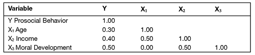
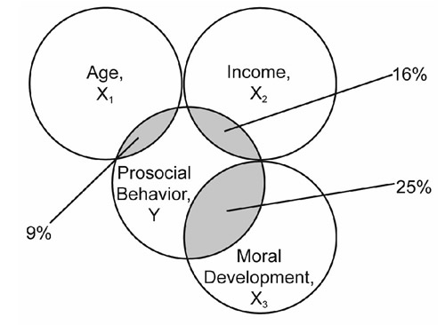
The X variables in Table 13.6 display the same correlations with Y as previously displayed in Table 13.5. However, in most cases this does not mean that the linear combination of the three X variables still accounts for the same total percentage of variance in Y. Remember that in Table 13.5 the X variables are not correlated with one another, whereas in Table 13.6 there is now a correlation between age and income, and between income and moral development. These correlations can decrease the total variance in Y accounted for by the X variables. The Venn diagram in Figure 13.5 illustrates these correlations.

In Figure 13.5, plain gray areas represent variance in income that is accounted for by age only and moral development only. The white area with cross-hatching represents variance in prosocial behavior accounted for by income only.

Notice that each X variable individually still accounts for the same percentage of variance in prosocial behavior—age still accounts for 9%, income accounts for 16%, and moral development accounts for 25%.

Figure 13.5: Venn Diagram of Variance Accounted for by Correlated Predictors

Figure 13.5 shows that some of the X variables are now correlated with one another. The area of overlap between age and income (gray and gray with crosshatching) shows that age and income now share about 25% of their variance (the correlation between these variables was 0.50, and 0.502 = 0.25). In the same way, the area of overlap between income and moral development (also gray and gray with crosshatching) represents the fact that these variables share slightly less than 25% of their variance in common.

When there is correlation between some of the X variables, a portion of the variance in Y accounted for by one X is now also accounted for by another X. For example, consider X2, which is the income variable. By itself, income accounted for 16% of the variance in prosocial behavior. But notice how the circle for age overlaps part of the variance in Y accounted for by income (area with gray crosshatch). This means that some of the variance in Y that is accounted for by income is also accounted for by age. That is, the amount of variance in Y uniquely accounted for by income has decreased because of correlation between age and income.

The same is true when you consider the correlation between income and moral development. The circle for moral development overlaps part of the variance in Y accounted for by income (gray with crosshatching). Some of the variance in Y that was accounted for by income is now also accounted for by moral development.

Because age and income are correlated, there is redundancy between them in the prediction of Y. There is also redundancy between income and moral development in the prediction of Y. The result of correlation between the predictor variables is a decrease in the total amount of variance in Y accounted for by the linear combination of X variables.

Compare the Venn diagram for the situation in which the X variables were uncorrelated (Figure 13.4) to the Venn diagram for the situation in which there was some correlation between the X variables (Figure 13.5). When the X variables were not correlated among themselves, they accounted for 50% of the variance in Y. Notice that the area in Y that overlaps with the X variables in Figure 13.5 is smaller, showing that the X variables account for less of the total variance in Y when they are correlated. The greater the correlation between the X variables, the smaller the amount of unique variance in Y accounted for by each individual X variable, and hence the smaller the total variance in Y that is accounted for by the combination of X variables.

The meaning of unique variance can be understood by looking at the crosshatched area in the Venn diagram in Figure 13.5. The two sections of the gray crosshatched area identify the variance in Y that is accounted for by income and age together, and by income and moral development together. The white crosshatched area shows the variance in Y that is uniquely accounted for by income. This area is quite small, which indicates that income accounts for very little variance in prosocial behavior that is not already accounted for by age and moral development.

One practical implication arising from this scenario is that the amount of variance accounted for in a response variable is larger to the extent that the following two conditions hold:

• the predictor variables shows strong correlations with the response variable
• the predictor variables demonstrate weak correlations with each other

These conditions hold true in general but they do not apply to the special case of a suppressor variable, which is discussed next.

A second implication is that there is generally a point of diminishing returns when adding new X variables to a multiple regression equation. Because so many predictor variables in social science research are correlated, only the first few predictors in a predictive equation are likely to account for meaningful amounts of unique variance in a response. Variables that are subsequently added tend to account for smaller and smaller percentages of unique variance. At some point, predictors added to the equation account for only negligible amounts of unique variance. For this reason, most multiple regression equations in social science research contain a relatively small number of variables, usually 2 to 10.

When Correlated Predictors Include a Suppressor Variable

The preceding section describes the results that you can usually expect to observe when regressing a response variable on multiple correlated predictor variables. However, suppressor variables are a special case in which the preceding generalizations do not hold. Although genuine suppressor variables are somewhat rare in the social sciences, it is important to understand the concept, so that you can recognize a suppressor variable.

A suppressor variable is a predictor variable that improves the predictive power of a multiple regression equation by controlling for unwanted variation that it shares with other predictors. Suppressor variables typically display these characteristics:

• zero or near-zero correlations with the response
• moderate-to-strong correlations with at least one other predictor variable

Suppressor variables are interesting because, even though they can display a bivariate correlation with the response variable of zero, adding them to a multiple regression equation can result in a meaningful increase in R2 for the model, which violates the generalizations given in the preceding section.

To understand how suppressor variables work, consider this fictitious example. Imagine that you want to identify variables that can be used to predict the success of firefighters. To do this, you conduct a study with a group of 100 firefighters. For each participant, you obtain a Firefighter Success Rating, which indicates how successful this person has been as a firefighter. These ratings are on a scale of 1 to 100, with higher ratings indicating greater success.

To identify variables that might be useful in predicting these success ratings, each firefighter completes a number of paper-and-pencil tests. One of these is a Firefighter Knowledge Test. High scores on this test indicate that the participant possesses the knowledge needed to operate a fire hydrant, enter a burning building safely, and perform other tasks related to firefighting. A second test is a Verbal Ability Test. This test has nothing to do with firefighting—high scores indicate that the participant has a good vocabulary and other verbal skills.

The three variables in this study could be represented with the following symbols:

Y = Firefighter Success Ratings (the response variable)

Xp = Firefighter Knowledge Test (the predictor variable of interest)

Xs = Verbal Ability Test (the suppressor variable)

Imagine that you perform some analyses to understand the nature of the relationship among these three variables. First, you compute the Pearson correlation coefficient between the Firefighter Knowledge Test and the Verbal Ability Test, and find that r = 0.40. This is a moderately strong correlation and makes sense because both firefighter knowledge and verbal ability are assessed by a paper-and-pencil testing method. To some extent, getting a high score on either of these tests requires that the participant be able to read instructions, read questions, read possible responses, and perform other verbal tasks. The results of the two tests are correlated because scores on both tests are influenced by the participant’s verbal ability.

Next, you perform a series of regressions, in which Firefighter Success Ratings (Y) is the response, to determine how much variance in this response is accounted for by various regression equations. This is what you learn:

• When the regression equation contains only the Verbal Ability Test, it accounts for 0% of the variance in Y.
• When the regression equation contains only the Firefighter Knowledge Test, it accounts for 20% of the variance in Y.
• When the regression equation contains both the Firefighter Knowledge Test and the Verbal Ability test, it accounts for 25% of the variance in Y.

Finding that the Verbal Ability Test accounts for none of the variance in Firefighter Success Ratings makes sense, because firefighting (presumably) does not require a good vocabulary or other verbal skills.

The second finding that the Firefighter Knowledge Test accounts for a respectable 20% of the variance in Firefighter Success Ratings also makes sense as it is reasonable to expect more knowledgeable firefighters to be rated as better firefighters.

However, you run into a difficulty when trying to make sense of finding that the equation with both the Verbal Ability Test and the Firefighter Knowledge Test accounts for 25% of the variance in Y. How is it possible that the combination of these two variables accounts for 25% of the variance in Y when one accounted for only 20% and the other accounted for 0%?

The answer is that, in this situation, the Verbal Ability Test is serving as a suppressor variable. It is suppressing irrelevant variance in scores on the Firefighter Knowledge Test, thus purifying the relationship between the Firefighter Knowledge Test and Y. Here is how it works. At least two factors influence scores on the Firefighter Knowledge Test—their actual knowledge about firefighting and their verbal ability (ability to read instructions). Obviously, the first of these two factors is relevant for predicting Y, whereas the second factor is not. Because scores on the Firefighter Knowledge Test are to some extent contaminated by the effects of the participant’s verbal ability, the actual correlation between the Firefighter Knowledge Test and Firefighter

Success Ratings is somewhat lower than it would be if you could somehow purify Knowledge Test scores of this unwanted verbal factor. That is exactly what a suppressor variable does.

In most cases, a suppressor variable is given a negative regression weight in a multiple regression equation. These weights are discussed in more detail later in this chapter. Partly because of the negative weight, including the suppressor variable in the equation adjusts each participant’s predicted score on Y so that it comes closer to that participant’s actual score on Y. In the present case, this means that a participant who scores above the mean on the Verbal Ability Test will have a predicted score on Y adjusted downward to penalize for scoring high on this irrelevant predictor. Alternatively, a participant who scores below the mean on the Verbal Ability Test has a predicted score on Y that is adjusted upward. Another way of thinking about this is to say that a person applying to be a firefighter who has a high score on the Firefighter’s Knowledge Test but a low score on the Verbal Ability Test would be preferred over an applicant with a high score on the Knowledge Test and a high score on the Verbal Test because the second candidate’s score on the Knowledge Test was probably inflated due to having good verbal skills.

The net effect of these corrections is improved accuracy in predicting Y. This is why you earlier found that R2 is 0.25 for the equation that contains the suppressor variable, but only 0.20 for the equation that does not contain it.

The possible existence of suppressor variables has implications for multiple regression analyses. For example, when attempting to identify variables that would make good predictors in a multiple regression equation, it is clear that you should not base the selection exclusively on the bivariate (Pearson) correlations between the variables. For example, even if two predictor variables are moderately or strongly correlated, it does not necessarily mean that they are always providing redundant information. If one of them is a suppressor variable, then the two variables are not entirely redundant. That noted, predictor variables that are highly correlated with other variables can cause problems with the analysis because of this collinearity. See the description of collinearity in the “Assumptions Underlying Multiple Regression” section in this chapter.

In the same way, a predictor variable should not be eliminated from consideration as a possible predictor just because it displays a low bivariate correlation with the response. This is because a suppressor variable may display a zero bivariate correlation with Y even though it could substantially increase R2 if added to a multiple regression equation. When starting with a set of possible predictor variables, it is generally safer to begin the analysis with a multiple regression equation that contains all predictors, on the chance that one of them serves as a suppressor variable. Choosing an optimal subset of predictor variables from a larger set is complex and beyond the scope of this book.

To provide a sense of perspective, true suppressor variables are somewhat rare in social science research. In most cases, you can expect your data to behave according to the generalizations made in the preceding section when there are no suppressors. In most cases, you will find that R2 is larger to the extent that the X variables are more strongly correlated with the Y variables, and are less strongly correlated with one another. To learn more about suppressor variables, see Pedhazur (1982).

The Uniqueness Index

A uniqueness index represents the percentage of variance in a response that is uniquely accounted for by a given predictor variable, above and beyond the variance accounted for by the other predictor variables in the equation. A uniqueness index is one measure of an X variable’s importance as a predictor—the greater the amount of unique variance accounted for by a predictor, the greater its usefulness.

The Venn diagram in Figure 13.6 illustrates the uniqueness index for the predictor variable income. It is identical to Figure 13.5 with respect to the correlations between income and prosocial behavior and the correlations between the three X variables. However, in Figure 13.6 only the area that represents the uniqueness index for income is shaded. You can see that this area is consistent with the previous definitions, which stated that the uniqueness index for a given variable represents the percentage of variance in the response (prosocial behavior) that is accounted for by the predictor variable (income) over and above the variance accounted for by the other predictors in the equation (age and moral development).

Figure 13.6: Venn Diagram: Uniqueness Index for Income

It is often useful to know the uniqueness index for each X variable in the multiple regression equation. These indices, along with other information, help explain the nature of the relationship between the response and the predictor variables. The Fit Model platform in JMP computes the uniqueness index and its significance level for each effect in the model.

Multiple Regression Coefficients

The b weights discussed earlier in this chapter referred to nonstandardized multiple regression coefficients. A multiple regression coefficient for a given X variable represents the average change in Y that is associated with a one-unit change in one X variable while holding constant the remaining X variables. Holding constant means that the multiple regression coefficient for a given predictor variable is an estimate of the average change in Y that would be associated with a one-unit change in that X variable if all participants had identical scores on the remaining X variables.

When conducting multiple regression analyses, researchers often want to determine which of the X variables are important predictors of the response. It is tempting to review the multiple regression coefficients estimated in the analysis and use these as indicators of importance. According to this logic, a regression coefficient represents the amount of weight that is given to a given X variable in the prediction of Y.

Nonstandardized Compared to Standardized Coefficients

However, caution must be exercised when using multiple regression coefficients in this way. Two types of multiple regression coefficients are produced in the course of an analysis—nonstandardized coefficients and standardized coefficients.

• Nonstandardized multiple regression coefficients (b weights) are the coefficients that are produced when the data analyzed are in raw score form. Raw score variables have not been standardized in any way. This means that different variables can have very different means and standard deviations. For example, the standard deviation for X1 might be 1.35, while the standard deviation for X2 might be 584.20.

In general, it is not appropriate to use the relative size of nonstandardized regression coefficients to assess the relative importance of predictor variables because the relative size of a nonstandardized coefficient for a given predictor variable is influenced by the size of that predictor’s standard deviation. Variables with larger standard deviations tend to have smaller nonstandardized regression coefficients while variables with smaller standard deviations tend to have larger regression coefficients. Therefore, the size of nonstandardized coefficients usually tells little about the importance of the predictor variables.

• Nonstandardized coefficients are often used to calculate participants’ predicted scores on Y. For example, an earlier section presented a multiple regression equation for the prediction of prosocial behavior in which X1 = age, X2 = income, and X3 = moral development. That equation is reproduced here.

= (0.10)X1 + (0.25)X2 + (1.10)X3 + (–3.25)

In this equation, the nonstandardized multiple regression coefficient for X1 is 0.10, the coefficient for X2 is 0.25, and so forth. If you have a participant’s raw scores on the three predictor variables, these values can be inserted in the preceding formula to compute that participant’s estimated score on Y. The resulting value is also in raw score form. It is an estimate of the number of prosocial acts you expect the participant to perform over a six-month period.

In summary, you should not refer to the nonstandardized regression coefficients to assess the relative importance of predictor variables. A better alternative (though still not perfect) is to refer to the standardized coefficients. Standardized multiple regression coefficients (called Beta weights in this book) are produced when the data are in a standard score form. Standard score form (or z score form) means that the variables have been standardized so that each has a mean of 0 and a standard deviation of 1. This is important because all variables (Y variables and X variables alike) now have the same standard deviation (a standard deviation of 1). This means they are now measured on the same scale of magnitude. Variables no longer will display large regression coefficients simply because they have small standard deviations. To some extent, the size of standardized regression coefficients does reflect the relative importance of the various predictor variables. These coefficients should be consulted to interpret the results of a multiple regression analysis.

For example, assume that the analysis of the prosocial behavior study produced the following multiple regression equation with standardized coefficients:

= (0.70)X1 + (0.20)X2 + (0.20)X3

In the preceding equation, X1 shows the largest standardized coefficient, which can be interpreted as evidence that it is a relatively important predictor variable, compared to X2 and X3.

You can see that the preceding equation, like all regression equations with standardized coefficients, does not contain an intercept constant. This is because the intercept is always equal to 0 in a standardized equation. If a researcher presents a multiple regression equation in a research article but does not indicate whether it is a standardized or a nonstandardized equation, look for the intercept constant. If there is an intercept in the equation, it is almost certainly a nonstandardized equation. If there is no intercept, it is probably a standardized equation. Also, remember that the lowercase letter b is often used to represent nonstandardized regression coefficients, while standardized coefficients are referred to as Beta weights (sometimes represented by the capital letter B or the Greek letter ).

Interpretability of Multiple Regression Coefficients

The preceding section noted that standardized coefficients reflect the importance of predictors only to some extent.

Regression coefficients can be difficult to interpret because when multiple regression using the same variables is performed on data from more than one sample, different estimates of the multiple regression coefficients are often obtained in the different samples. This is the case for standardized as well as nonstandardized coefficients.

For example, assume that you recruit a sample of 50 participants, measure the variables discussed in the preceding section (prosocial behavior, age, income, moral development), and compute a multiple regression equation in which prosocial behavior is the response and the remaining variables are predictors (assume that age, income, and moral development are X1, X2, and X3, respectively). With the analysis completed, it is possible that your output would reveal the following standardized regression coefficients for the three predictors:

= (0.70)X1 + (0.20)X2 + (0.20)X3

The relative size of the coefficients in the preceding equation suggests that X1 (with a Beta weight of 0.70) is the most important predictor of Y, while X2 and X3 (each with Beta weights of 0.20) are much less important.

However, if you replicate your study with a different group of 50 participants, you would compute different Beta weights for the X variables. For example, you might obtain:

= (0.30)X1 + (0.50)X2 + (0.10)X3

In the second equation, X2 has emerged as the most important predictor of Y, followed by X1 and X3.

When the same study is performed on different samples, researchers usually obtain coefficients of different sizes. This means that the interpretation of these coefficients must always be made with caution. Specifically, multiple regression coefficients become increasingly unstable as the analysis is based on smaller samples and as the X variables become more correlated with one another. Unfortunately, much of the research carried out in the social sciences involves the use of small samples and correlated X variables. For this reason, the standardized regression coefficients (Beta weights) are only a few of the pieces of information to review when assessing the relative importance of predictor variables. The use of these coefficients should be supplemented with a review of the simple bivariate correlations between the X variables and Y and the uniqueness indices for the standardized X variables. The following sections show how to do this.

Example: A Test of the Investment Model

Fictitious data from a correlational study based on the investment model (Rusbult, 1980a, 1980b) illustrates the statistical procedures in this chapter. Recall that the investment model data was used to illustrate a number of other statistical procedures in previous chapters.

The investment model identifies a number of variables believed to predict a person’s level of commitment to a romantic relationship (as well as to other types of relationships). Commitment refers to the individual’s intention to maintain the relationship and remain with a current partner. One version of the investment model asserts that commitment is affected by the following four variables:

• Rewards: the number of good things that the participant associates with the relationship—the positive aspects of the relationship
• Costs: the number of bad things or hardships associated with the relationship
• Investment Size: the amount of time and personal resources that the participant has put into the relationship
• Alternative Value: the attractiveness of the participant’s alternatives to the relationship—the attractiveness of alternative romantic partners

The illustration in Figure 13.7 shows the hypothesized relationship between commitment and these four predictor variables.

Figure 13.7: One Version of the Investment Model

If the four predictor variables in Figure 13.7 do have a causal effect on commitment, it is reasonable to assume that they should also be useful for predicting commitment in a simple correlational study. Therefore, the present study is correlational in nature and uses multiple regression procedures to assess the nature of the predictive relationship between these variables. If the model survives this test, you might then want to follow it up by performing a new study to test the proposed causal relationships between the variables—perhaps a true experiment. However, the present chapter focuses only on multiple regression procedures.

Overview of the Analysis

To better understand the nature of the relationship between the five variables presented in Figure 13.7, the data are analyzed using several JMP platforms.

First, The Multivariate platform computes Pearson correlations between variables. Simple bivariate statistics are useful for understanding the big picture.

Next, the Fit Model platform performs a multiple regression in which commitment is simultaneously regressed on the predictor variables. This provides a number of important pieces of information.

• First, you determine whether there is a significant relationship between commitment and the linear combination of predictors. You want to know if there is a significant relationship between commitment and the four variables taken as a group.
• You can also review the multiple regression coefficients for each of the predictors to determine which are statistically significant and which standardized coefficients are relatively large.
• Examine the uniqueness of each predictor to see which variables account for a significant amount of variation in the response when included in the regression equation.
• The Stepwise platform gives a multiple regression analysis for every possible combination of predictor variables. From these results you can determine the amount of variance in commitment accounted for any combination of predictor variables. These results are the difference in R2 values between the full model and the model that is reduced by one or more predictors. Stepwise gives statistical tests that determine which of the uniqueness indices are significantly different from zero.

Gathering Data

Assume that you conduct a study of 48 college students who are currently involved in romantic relationships. Each participant completes a 24-item questionnaire designed to assess the five investment model constructs—commitment, rewards, costs, investment size, and alternative value.

Each investment model construct is assessed with four questions. For example, the following four items assess the commitment construct:

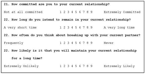
Notice that a higher response number (such as 8 or 9) indicates a higher level of commitment, whereas a lower response number (such as 1 or 2) indicates a lower level of commitment. The sum of these four items for a participant give a single score that reflects that participant’s overall level of commitment. This cumulative score serves as the commitment variable in your analyses. Scores on this variable can range from 4 to 36 with higher values indicating higher levels of commitment.

Each of the remaining investment model constructs are assessed the same way. The sum of four survey items creates a single overall measure of the construct. Scores can range from 4 to 36 and higher scores indicate higher levels of the construct being assessed.

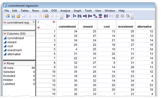
The JMP Data Table

The summarized (fictitious) data are in the JMP data table called commitment regression.jmp, which is shown in Figure 13.8. There are scores for variables commitment, reward, cost, investment, and alternative, for 48 participants.

Assume the scores in the Commitment Regression table were obtained as follows:

• Forty-eight participants completed a 24-item questionnaire designed to evaluate commitment to an existing relationship. In particular, five sets of four items assessed five commitment constructs. The score for a construct is the sum of its four items.
• The sum of the items for five of the constructs, commitment, reward, cost, investment, and alternative, are the scores in the commitment regression data table for each of the 48 participants.

Figure 13.8: Partial Listing of the Commitment Regression Data Table

Computing Simple Statistics and Correlations

It is often appropriate to begin a multiple regression analysis by computing simple univariate statistics on the study’s variables, and all possible bivariate correlations between them. A review of these statistics and correlations can help you understand the big picture concerning relationships between the response variable and the predictor variables and among the predictor variables themselves.

Univariate Statistics

Use the Distribution platform to look at univariate statistics on the study variables. Chapter 4, “Exploring Data with the Distribution Platform,” describes the Distribution platform in detail. To see simple statistics,

Choose Analyze > Distribution.

When the launch dialog appears, select all the variables in the variable selection list, and click Y, Columns in the dialog to see them in the analysis list.

Click OK in the launch dialog to see the Distribution results.

The platform results in Figure 13.9 show only the Quantiles and Moments tables. The Histograms and Outlier Box plots are not shown here, but offer a visual approach to identifying possible outliers in the data.

These distribution results are discussed in the “Review Simple Statistics and Correlation Results” section.

Figure 13.9: Univariate Statistics on Study Variables

Bivariate Correlations

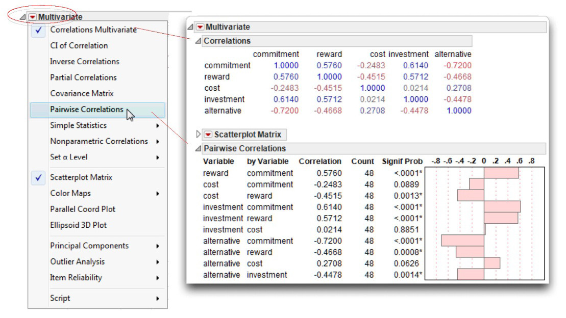
Chapter 5, “Measures of Bivariate Association,” discussed using the Multivariate platform to compute correlations. This analysis proceeds the same way. With the Commitment Regression table active (the front-most table),

Choose Analyze > Multivariate Methods > Multivariate.

When the launch dialog appears, select all the variables in the variable selection list, and click Y, Columns in the dialog to see them in the analysis list.

Click OK in the launch dialog to see the initial Multivariate results.

In the initial results window, close the Scatterplot Matrix, and choose Pairwise Correlations from the menu on the Multivariate title bar to see the results shown in Figure 13.10.

Figure 13.10: Bivariate Correlations and Simple Statistics for All Study Variables

Review Simple Statistics and Correlation Results

Step 1: Make sure everything looks reasonable. It is always important to review descriptive statistics to help verify that there are no obvious errors in the data table. The Distribution platform results in Figure 13.9 give tables of basic univariate statistics.

The Moments table gives means, standard deviations, and other descriptive statistics for the five study variables, and the Quantiles table lists values for common percentiles. It is easy to verify that all of the figures are reasonable. In particular, check the Minimum and Maximum values for evidence of problems. The lowest score that a participant could possibly receive on any variable was 4. If any variable displays a Minimum score below 4, an error must have been made when entering the data. Similarly, no valid score in the Maximum column should exceed 36.

Step 2: Determine the size of the sample producing the correlations. The N in the Moments table shows that all computations were completed for 48 observations. If any variable had a different number of observations associated with it (had missing values), then all simple statistics involving that variable are based on its reduced N value. Observations with missing values are not used for computations of any correlations in the Correlations table. These Pearson product-moment correlations are based only on observations that have values for all variables. If there are missing values, the Pairwise Correlations table shows correlations based on all nonmissing values for each pair of variables, and indicates the N for each pairwise correlation. Because there were no missing values in this example, the values in the Correlations table and in the Pairwise Correlations table are the same.

Step 3: Review the correlation coefficients. The correlations among the five variables appear in the 5 by 5 matrix at the top of the Multivariate results in Figure 13.10. In this matrix, where the row for one variable intersects with the column of a second variable, you find the cell that gives the correlation coefficient for these variables. The Pairwise Correlations table shows the probabilities associated with each correlation.

For example, the correlation between commitment (the response) and reward is 0.576. The p-value associated with this correlation, seen in the Pairwise Correlations table, is less than 0.0001, which means there is less than 1 chance in 10,000 of obtaining a coefficient this large by chance alone in another random sample of the same size. In other words, this correlation of 0.576 is statistically significant at the 0.0001 level.

Interpret the Correlations

The correlations in the commitment column of the Correlations table tell you about the pattern of bivariate correlations between commitment and the four predictors. Notice that commitment has a positive correlation with reward and investment. As you expect, participants who report higher levels of rewards and investment size also report higher levels of commitment. However, commitment has negative relationships with cost and alternative. This is also reasonable as participants who report higher levels of costs and alternative value report lower levels of commitment. Each of these correlations is in the direction predicted by the investment model (see Figure 13.7).

Notice that some predictors are more strongly related to commitment than others. Specifically, alternative displays the strongest correlation at –0.72, followed by investment (0.61) and reward (0.58). These correlations are statistically significant at the 0.0001 level.

The correlation between commitment and cost is lower at approximately –0.25 and is not statistically significant (p = 0.0889). Based on these results, you could not reject the null hypothesis that commitment and cost are uncorrelated in the population.

The correlations in Figure 13.10 also give important information about the correlations among the four predictor variables. When using multiple regression, an ideal predictive situation is one in which each predictor variable displays a relatively strong correlation with the response, while the predictor variables display relatively weak correlations among themselves as discussed earlier.

With this in mind, the correlations presented in Figure 13.10 indicate that the association among variables in the current data table is less than ideal. It is true that three of the predictors display relatively strong correlations with commitment, but it is also true that most of the predictors display relatively strong correlations with each other. Notice that r = –0.45 for reward and cost, r = 0.57, between reward and investment, and r = –0.47 for reward and alternative. These correlations are moderately large as is the correlation between investment and alternative. Moderate correlations sometimes result in nonsignificant multiple regression coefficients for at least some predictor variables as seen in the analyses reported in the following section.

Estimating the Full Multiple Regression Equation

The Fit Model platform in JMP can perform multiple regression analysis. This procedure estimates multiple regression coefficients for the various predictors, calculates R2, tests for significance, and shows additional information relevant to the analysis.

Using the Fit Model Platform

Chapters 8, 9, and 10 showed how to use the Fit Model platform for analysis of variance, analysis of factorial designs, and multivariate analysis of variance. The process is the same for doing multiple regression.

Select Analyze > Fit Model.

When the Fit Model dialog appears, select commitment as Y and the four predictors as effects as shown in Figure 13.11.

Click Run in the dialog to see the multiple regression analysis.

Note: It is important to remember that JMP uses the modeling type of the analysis variables to determine the correct analysis. When the response (Y) variable and all the predictors (X variables or effects) are continuous numeric variables, the Fit Model platform automatically selects a standard least squares multiple regression analysis unless you specify otherwise.

Figure 13.11: Fit Model Dialog for Multiple Regression

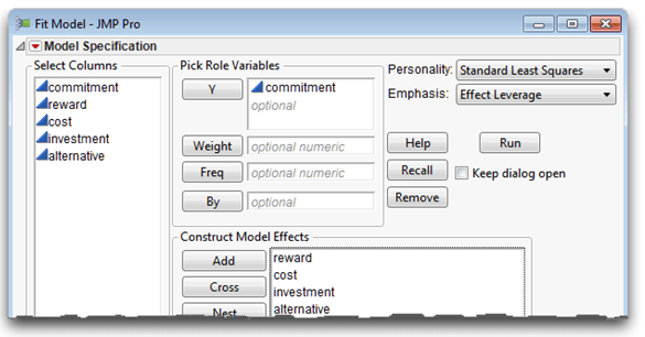
Review the Multiple Regression Results

When you click Run in the Fit Model dialog, you see the results shown in
Figure 13.12.

Figure 13.12: Multiple Regression Results

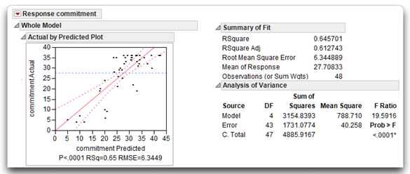
Use the following guidelines to review these results:

Step 1: Make sure that everything looks reasonable. The title bar of the results shows that the response variable is commitment. The value for Observations in the Summary of Fit table shows that there were 48 participants. In the Analysis of Variance table, the DF heading (degrees of freedom) shows that the C. total (corrected total) is 47, which is equal to N – 1, where N is the total number of participants who provided usable data for the analysis. There are four predictor variables so there should be 4 degrees of freedom for the model, as shown by the DF for Model in the Analysis of Variance table.

Step 2: Review the Whole Model results. Figure 13.12 shows the initial results of the multiple regression. The Actual by Predicted Plot and Analysis of Variance table tell you if the linear combination of predictor variables accounts for a significant amount of variation in the response, commitment.

Note that the Actual by Predicted leverage plot shows you at a glance that the multiple regression model is statistically significant. The horizontal reference line on the plot represents the condition that all effects are zero. The fitted line and its confidence lines cross the reference line (do not encompass the reference line), which indicates a significant regression model.

To test the null hypothesis that all effects are zero, look at the line labeled Model in the Analysis of Variance table. You see an F value (F Ratio) of 19.59 and its associated probability (Prob > F) is less than 0.0001. Remember that the p-value is the probability that you would obtain an F-value this large or larger if the null hypothesis were true. In this case, the p-value is very small (< 0.0001), so you reject the null hypothesis and conclude that the predictors, taken as a group, do account for a significant amount of variation in the response.

Step 3: Review the obtained value of R2. You see the R2 value in two places—the Actual by Predicted plot in Figure 13.12 lists Rsq = 0.65, and the Summary of Fit table give Rsquare as 0.645701. Recall that this R2 value indicates the percent of variance in the response variable accounted for by the linear combination of predictor variables. The R2 of 0.6457 indicates that the linear combination of reward, cost, investment, and alternative accounts for (explains) about 65% of the variance in commitment. The significance test for Model, discussed previously, also tests the hypothesis R2 = 0.

The regression analysis determines whether the linear combination of predictor variables accounts for a significant amount of variance in the response. You also want to determine whether the predictors account for a large enough amount of variance to be considered meaningful. How large must an R2 value be to be considered meaningful? That depends, in part, on what has been found in prior research concerning the response variable being investigated. If, for example, predictor variables in earlier investigations have routinely accounted for 50% of the variance in the response but the predictors in your study have accounted for only 10%, these new findings might not be viewed as being very important. On the other hand, if the predictors of earlier studies have routinely accounted for only 5% of the variance but the variables of your study have accounted for 10%, this might be considered a meaningful amount of variance.

This issue of statistical significance versus percentage of variance accounted for is important because it is possible to obtain an R2 value that is very small (say, 0.03), but is still statistically significant. This occurs when analyzing data from very large samples.

Therefore, when assessing the importance of your findings, always review both the statistical significance of the model equation, and the total amount of variance accounted for by the predictors.

Step 4: Review the adjusted value of R2. The Summary of Fit table also lists the adjusted R2, labeled Rsquare Adj. The adjusted R2 is a ratio of mean squares instead of a ratio of sums of squares, and therefore uses degrees of freedom in its calculations. For this reason it is more comparable over models with different numbers of parameters (different degrees of freedom). The adjusted R2 tends to favors more parsimonious solutions (models with fewer effects). Also, the value of R2 obtained with a given sample often overestimates the population value of R2, while the adjusted R2 corresponds more closely to the population value. For this reason, the adjusted R2 is usually smaller than the standard R2.

Step 5: Review the intercept and nonstandardized regression coefficients. The parameter estimates in the Parameter Estimates table shown here are the terms that constitute the multiple regression equation.

• The first column of information, called Term, lists the names of the terms in the regression equation—the intercept and the four predictor variables (reward, cost, investment, and alternative).
• The column called Estimate lists the intercept estimate and the nonstandardized multiple regression coefficients for the predictors. The Intercept is 20.038, the nonstandardized regression coefficient for Reward is 0.279, for Cost is –0.106, and so forth. You can write the multiple regression equation in this way:

= 0.279(reward) – 0.106(cost) + 0.523(investment) – 0.679(alternative) + 20.038

Remember that the multiple regression coefficient for a given predictor indicates the amount of change in Y associated with a one-unit change in that predictor while holding the remaining predictors constant. Nonstandardized coefficients represent the change observed when the variables are in raw score form (the different variables have different means and standard deviations). The nonstandardized regression equation is used to predict participants’ scores on commitment so that the resulting scores will be on the same scale of magnitude as observed with the raw data. However, the coefficients in this equation cannot be used to assess the relative importance of the predictor variables.

Step 6: Review the leverage plots for the regression coefficients. Researchers usually want to determine whether regression coefficients for the various predictor variables are significantly different from zero. A zero coefficient for a predictor variable indicates the variable has no effect on the response. A statistically significant coefficient suggests that the corresponding predictor variable is an important predictor of the response.

The Fit Model results include effect leverage plots, which tell you at a glance whether effects are significant. Figure 13.13 shows leverage plots for the four effects in the multiple regression analysis.

Figure 13.13: Leverage Plots for Four Effects in the Multiple Regression Analysis

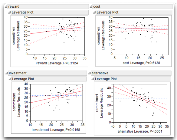
Leverage plots were discussed in Chapter 9, “Factorial ANOVA with Two Between-Subjects Factors.” The leverage plot shows the line of fit, its 95% confidence curves, and the horizontal mean reference line that represents the null hypothesis. If the 95% curves cross the horizontal mean reference line, then the model fits better than the simple mean fit. If the curves do not cross the mean line—if they include or encompass the mean line—the model line fits the data no better than the mean line itself. Note in Figure 13.13 that neither reward nor cost appears significant in the leverage plots, but investment and alternative are statistically significant.

Step 7: Examine the significance tests for the coefficients. The Parameter Estimates table gives details about the regression coefficients. The column called t Ratio lists a t test for the intercept and each predictor variable. These test the null hypothesis that the regression coefficient is equal to zero. The p-value corresponding to each t statistic is in the column Prob > |t|.

For example, the nonstandardized regression coefficient estimate for reward is 0.279, its t test value is 1.02, and the corresponding p-value is 0.3124. Because this p-value is greater than 0.05, you cannot reject the null hypothesis and conclude that the regression coefficient for reward is not significantly different from zero. However, investment has a nonstandardized regression coefficient of 0.523. The t-value for this coefficient is 2.49 with a corresponding p-value of 0.0168. Because this value is less than 0.05, you reject the null hypothesis and tentatively conclude that the coefficient for investment is significantly different from zero.

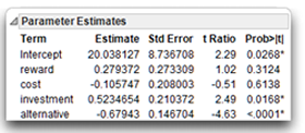
Recall that the statistical significance of a regression coefficient suggests that variable’s importance as a predictor. This statement includes a qualification to emphasize that caution must be used when interpreting statistical significance as evidence of a predictor’s importance. There are at least two reasons for this:

• First, multiple regression coefficients can be unstable and difficult to interpret when the sample size is small. Small sample sizes often produce inflated standard errors and correlation between predictor variables.
• Second, a multiple regression coefficient can be statistically significant even when the standardized coefficient is relatively small in absolute magnitude and has little predictive value. This is more likely to happen when sample sizes are very large.

For these reasons, the statistical significance of regression coefficients should be viewed as only one indicator of a variable’s importance and should always be combined with additional information such as the size of the standardized regression coefficients and uniqueness indices.

Step 8: Review the standardized regression coefficients (Beta weights). The values of nonstandardized regression coefficients often indicate little about the relative importance of predictor variables because the different predictors often have different scales of measurement. These differences affect the size of the nonstandardized coefficients. To avoid this difficulty, review the standardized multiple regression coefficients (Beta weights). Beta weights are the regression coefficients that result when all the variables are standardized to have mean of 0 and standard deviation of 1. It is appropriate to review the Beta weights when you want to compare the relative importance of predictor variables.

To include standardized regression coefficients (Beta weights) in the results, right-click anywhere in the Parameter Estimates table to see the menu shown in Figure 13.14. When you choose Std Beta from this menu, the standardized parameter estimates then appear in the Parameter Estimates table. Note that the intercept for this equation is 0—this is always the case with a standardized regression equation:

• the Beta weight for reward is 0.138
• the Beta weight for cost is –0.057
• the Beta weight for investment is 0.312
• the Beta weight for alternative is –0.500

Based on these findings, you can tentatively rank the predictors from most to least influential Y predictors as alternative, investment, reward, and cost.

Figure 13.14: Parameter Estimates Table with Standardized Beta

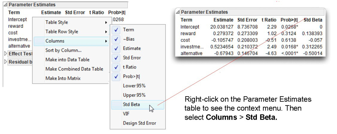
A more cautious approach to understanding the relative importance of predictor variables involves combining information from a variety of sources, including bivariate correlations, standardized regression coefficients, and the uniqueness indices.

The Parameter Estimates table (see Figure 13.14) does not report significance tests for the standardized regression coefficients because when the t test for the nonstandardized coefficient is significant, then the corresponding standardized coefficient for that variable is also significantly different from zero.

Uniqueness Indices for the Predictors

This section covers how to determine which predictors are most important in a multiple regression analysis.

The multiple regression analysis shown in the previous section also gives statistics that tell which effects are significant in the multiple regression equation. The Effect Tests table, which is shown in Figure 13.15, gives the F statistic for testing that each individual effect is zero. The F ratios, showing in the Effect Tests table, test the uniqueness index for each predictor.

The F-value is the ratio of the mean square for the effect and the mean square for error in the ANOVA. The effect’s mean square is its sum of squares divided by its degrees of freedom.

You can verify this by looking at the quantities in the tables shown in Figure 13.15. For example, the test for the alternative effect shows it is a significant predictor, with F = 21.4489 and p < 0.0001. That is,

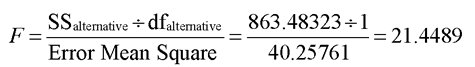
Note: To adjust the number of decimal places in any column of numbers showing in a report, double-click on the column of numbers and complete the Column Numeric Format dialog that appears.

This F ratio, showing in the Effect Tests table, tests the uniqueness index for alternative.

Figure 13.15: Effect Tests Table for Multiple Regression Analysis

Summarizing the Results

There are a number of different ways to summarize the results of a multiple regression analysis in a paper. The following summarized results use table formats that are fairly representative of those appearing in journals of the American Psychological Association (APA, 2003).

Correlation Results from the Multivariate Platform

It is usually desirable to present simple descriptive statistics, such as means and standard deviations, along with the correlation matrix. If reliability estimates (such as coefficient alpha estimates) are available for the predictors, they should be included in parentheses on the diagonal of the correlation matrix. The results for the present fictitious study are summarized in Table 13.8.

Table 13.8: Means, Standard Deviations, Correlations, and Alpha Reliability Estimates

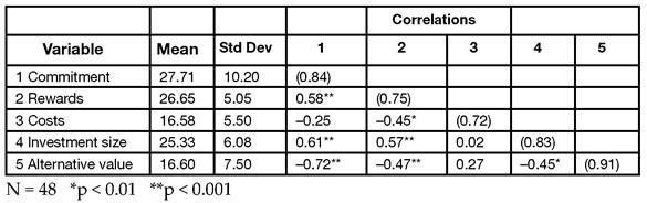
Regression Results from the Fit Model Platform

Depending on the nature of the research problem, it is sometimes feasible to report standardized regression coefficients (Beta weights, labeled Std Beta in the Parameter Estimates table) and the uniqueness indices in a single table as done in Table 13.9.

Table 13.9: Nonstandardized Estimates (b Weights), Beta Weights, and Uniqueness Indices from Multiple Regression Analyses

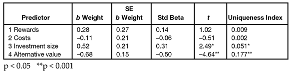
Note: R2 = 0.65, F(4, 43) = 19.59, p < 0.01 for predictor variables.

Getting the Big Picture

It is instructive to reflect on the big picture of your findings before you proceed to summarize them in text form. First, notice the bivariate correlations from Table 13.8. The correlations between commitment and rewards, between commitment and investment size, and between commitment and alternative value are all significant and in the predicted direction. Only the correlation between commitment and costs was nonsignificant. These findings provide partial support for the investment model.

A somewhat similar pattern of results can be seen in Table 13.9, which shows that the Beta weights and uniqueness indices for investment size and alternative value are both significant and in the predicted direction. However, unlike correlations, Table 13.9 shows that neither the Beta weight nor the uniqueness index for rewards is statistically significant. This might come as a surprise because the correlation between commitment and rewards was moderately strong at 0.58. With such a strong correlation, how could the multiple regression coefficient and uniqueness index for rewards be nonsignificant?

A possible answer may be found in the correlations of Table 13.8. Notice that the correlation between commitment and rewards is weaker than the correlation between commitment and either investment size or alternative value. In addition, the correlations between rewards and both investment size and alternative value are fairly substantial at r = 0.57 and r = –0.47, respectively. In short, amount of reward shares a great deal of variance in common with investment size and alternative value and is a poorer predictor of commitment. In this situation, it is unlikely that a multiple regression equation that already contains investment size and alternative value needs a variable like rewards to improve the accuracy of prediction. In other words, any variance in commitment that is accounted for by rewards has probably already been accounted for by investment size and alternative value. As a result, the rewards variable is redundant and so displays a nonsignificant Beta weight and uniqueness index.

Was this a real test of the investment model? It must be emphasized that the results of the investment model presented here are entirely fictitious and should not be viewed as legitimate tests of that conceptual framework. Most published studies of the investment model have been very supportive of its predictions. For representative examples of this research, interested readers are referred to Rusbult (1980a, 1980b), Rusbult and Farrell (1983), and Rusbult, Johnson, and Morrow (1986).

Formal Description of Results for a Paper

There are a number of ways to summarize the results of these analyses within the text of the paper. The amount of detail in the description should be dictated by the statistical sophistication of your audience. If the audience is likely to be familiar with the use of multiple regression, then less detail is needed.

The following format is fairly typical:

Results were analyzed using both bivariate correlation and multiple regression. Means, standard deviations, and Pearson correlations appear in Table 13.8. The bivariate correlations reveal three predictor variables that were significantly related to commitment: rewards (r = 0.58); investment size (r = 0.61); and alternative value (r = –0.72). All correlations are significant at p < 0.001, and all are in the expected direction. The correlation between costs and commitment is nonsignificant, at α = 0.05, with r = –0.25.
Using multiple regression, commitment scores were then regressed on the linear combination of rewards, costs, investment size, and alternative value. The equation containing these four variables accounted for 65% of observed variance in commitment,F(4, 43) = 19.60, p < 0.001, adjusted R2 = 0.61.
Beta weights (standardized multiple regression coefficients) and uniqueness indices were subsequently reviewed to assess the relative importance of the four variables in the prediction of commitment. The uniqueness index for a given predictor is the percentage of variance in the response accounted for by that predictor, beyond the variance accounted for by the other predictor variables. Beta weights and uniqueness indices are presented in Table 13.9.
Table 13.9 shows that only investment size and alternative value display significant Beta weights. Alternative value demonstrates a somewhat larger Beta weight at –0.50 (p < 0.001), while the Beta weight for investment size is 0.31 (p < 0.05). Both coefficients are in the predicted direction.
Findings regarding uniqueness indices correspond to those for Beta weights in that only investment size and alternative value display significant indices. Alternative value accounted for approximately 18% of the variance in commitment, beyond the variance accounted for by the other three predictors, F(1, 43) = 21.51, p < 0.001. In contrast, investment size accounts for only 5% of the unique variance in commitment, F(1, 43) = 6.20, p < 0.05.

Summary

This chapter provides an elementary introduction to multiple regression, one of the most flexible and powerful research tools in the social sciences. It discusses only the situation in which a response variable is being predicted from continuous predictor variables, all of which display a linear relationship with the response. At this time, you are ready to move on to a more comprehensive treatment of the topic that deals with curvilinear relationships, interactions between predictors, dummy coding, effect coding, and regression equations that contain both continuous and categorical predictor variables. Cohen, Cohen, West, and Aiken (2003), and Pedhazur (1982) provide authoritative treatments of these and other advanced topics in multiple regression. Also see Freund, Little, and Creighton (2003), and Sall, Lehman, Stephens, and Creighton (2012).

Appendix: Assumptions Underlying Multiple Regression

Level of measurement

For multiple regression, both the predictor variables and the response variable should be numeric continuous variables.

Random sampling

Each participant in the sample contributes one score on each predictor variable, and one score on the response variable. These sets of scores represent a random sample drawn from the population of interest.

Normal distribution of the response variable

For any combination of values on the predictor variables, the response variable should be normally distributed.

Homogeneity of variance

For any combination of values of the predictor variables, the response variable should demonstrate a constant variance.

Independent observations

A given observation should not be affected by (or related to) any other observation in the sample. For example, this assumption would be violated if the various observations represented repeated measurements taken from a single participant. It would also be violated if the study included multiple participants, some of whom contributed more than one observation to the data set (some participants contributed more than one set of scores on the response variable and predictor variables).

Linearity

The relationship between the response variable and each predictor variable should be linear. This means that the mean response scores at each value of a given predictor should fall on a straight line.

Errors of prediction

The errors of prediction should be normally distributed and the distribution of errors should be centered at zero. Errors of prediction associated with a given observation should not be correlated with those associated with the other observations. Errors of prediction should demonstrate a consistent variance. Errors of prediction should not be correlated with the predictor variables.

Absence of measurement error

The predictor variables should be measured without error. Pronounced violations of this assumption lead to underestimation of the regression coefficient for the corresponding predictor.

Absence of specification errors

The term specification error generally refers to situations in which the model represented by the regression equation is not theoretically tenable. In multiple regression, specification errors most frequently result from omitting relevant predictor variables from the equation or including irrelevant predictor variables in the equation. Specification errors also result when researchers posit a linear relationship between variables that are actually involved in a nonlinear relationship.

It is infrequent that all of these assumptions will be fully satisfied in applied research. Fortunately, regression analysis is generally robust against minor violations of most of these assumptions. However, it is less robust against violations of the assumptions involving independent observations, measurement error, or specification errors (Pedhazur, 1982).

In addition to considering the preceding assumptions, researchers are also advised to inspect their data for possible problems involving outliers or collinearity.

• An outlier is an unusual observation that does not fit the regression model well. Outliers are often the result of mistakes made when entering data, and can profoundly bias parameter estimates (such as regression coefficients). The Outlier analysis in the Multivariate platform could be used to detect possible outliers.
• As previously noted, collinearity exists when two or more predictor variables demonstrate a high degree of correlation, such as r > 0.90, with one another. Collinearity can cause regression coefficient estimates to fail to demonstrate statistical significance, be biased, or even demonstrate the incorrect sign. Cohen, Cohen, West, and Aiken (2003) discuss these problems, and show how to detect outliers, collinearity, and other problems sometimes encountered in regression analysis.

References

American Psychological Association. 2001. Publication Manual of the American Psychological Association, Fifth Edition. Washington, DC: American Psychological Association.

Cohen, J. 1992. “A Power Primer.” Psychological Bulletin, 112, 155–159.

Cohen, J., Cohen, P., West, S. G., and Aiken, L. S. 2003. Applied Multiple Regression/ Correlation Analysis for the Behavioral Sciences, Third Edition. Hillsdale, NJ: Lawrence Erlbaum.

Freund R., Little, R., and Creighton, L. 2003. Regression Using JMP. Cary, NC: SAS Institute Inc.

Hopkins, K. D., Glass, G. V., and Hopkins, B. R. 1987. Basic Statistics for the Behavioral Sciences. Englewood Cliffs, NJ: Prentice-Hall.

Pedhazur, E. J. 1982. Multiple Regression in Behavioral Research, Second Edition. New York: Holt, Rinehart, and Winston.

Rusbult, C. E. 1980a. “Commitment and Satisfaction in Romantic Associations: A Test of the Investment Model.” Journal of Experimental Social Psychology, 16, 172–186.

Rusbult, C. E. 1980b. “Satisfaction and Commitment in Friendships.” Representative Research in Social Psychology, 11, 96–105.

Rusbult, C. E., and Farrell, D. 1983. “A Longitudinal Test of the Investment Model: The Impact on Job Satisfaction, Job Commitment, and Turnover of Variations in Rewards, Costs, Alternatives, and Investments.” Journal of Applied Psychology, 68, 429–438.

Rusbult, C. E., Johnson, D. J., and Morrow, G. D. 1986. “Predicting Satisfaction and Commitment in Adult Romantic Involvements: An Assessment of the Generalizability of the Investment Model.” Social Psychology Quarterly, 49, 81–89.

Sall, J., Lehman, A., Stephens, M., and Creighton, L. 2012. JMP Start Statistics. Cary, NC: SAS Institute Inc.

SAS Institute Inc. 2012. Modeling and Multivariate Methods. Cary, NC: SAS Institute Inc.