
Let's plot a polynomial and its first-order derivative using the deriv() function with m as 1. We already did the first part in the previous Time for action section. We want two different line styles to discern what is what.
- Create and differentiate the polynomial:
func = np.poly1d(np.array([1, 2, 3, 4]).astype(float))
func1 = func.deriv(m=1)
x = np.linspace(-10, 10, 30)
y = func(x)
y1 = func1(x)
- Plot the polynomial and its derivative in two styles: red circles and green dashes. You cannot see the colors in a print copy of this book, so you will have to try the code out for yourself:
plt.plot(x, y, 'ro', x, y1, 'g--')
plt.xlabel('x')
plt.ylabel('y')
plt.show()
The graph with polynomial coefficients
1,2,3, and4is as follows: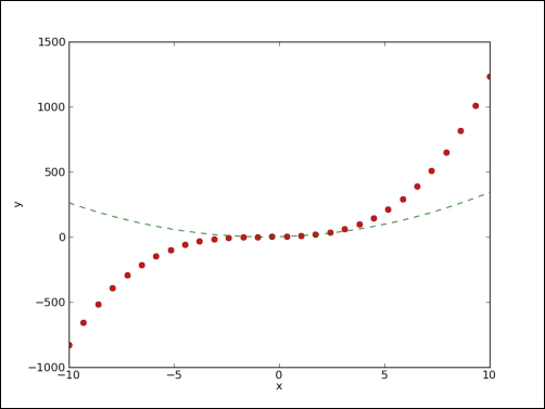
We plotted a polynomial and its derivative using two different line styles and one call of the plot() function (see polyplot2.py):
import numpy as np
import matplotlib.pyplot as plt

func = np.poly1d(np.array([1, 2, 3, 4]).astype(float))
func1 = func.deriv(m=1)
x = np.linspace(-10, 10, 30)
y = func(x)
y1 = func1(x)

plt.plot(x, y, 'ro', x, y1, 'g--')
plt.xlabel('x')
plt.ylabel('y')
plt.show()..................Content has been hidden....................
You can't read the all page of ebook, please click here login for view all page.