
Often we are more interested in the trend of a data sample than in detrending it. We can still get the trend back easily after detrending. Let's do that for one year of price data for QQQ.
- Write code that gets the close price and corresponding dates for QQQ:
today = date.today() start = (today.year - 1, today.month, today.day) quotes = quotes_historical_yahoo("QQQ", start, today) quotes = np.array(quotes) dates = quotes.T[0] qqq = quotes.T[4] - Detrend the signal:
y = signal.detrend(qqq)
- Create month and day locators for the dates:
alldays = DayLocator()
months = MonthLocator()
- Create a date formatter that creates a string of month name and year:
month_formatter = DateFormatter("%b %Y") - Create a figure and subplot:
fig = plt.figure()
ax = fig.add_subplot(111)
- Plot the data and underlying trend by subtracting the detrended signal:
plt.plot(dates, qqq, 'o', dates, qqq - y, '-')
- Set the locators and formatter:
ax.xaxis.set_minor_locator(alldays)
ax.xaxis.set_major_locator(months)
ax.xaxis.set_major_formatter(month_formatter)
- Format the x-axis labels as dates:
fig.autofmt_xdate()
plt.show()
The following figure shows the QQQ prices with a trend line:
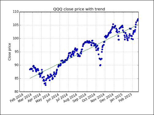
We plotted the closing price for QQQ with a trend line (see trend.py):
from matplotlib.finance import quotes_historical_yahoo
from datetime import date
import numpy as np
from scipy import signal
import matplotlib.pyplot as plt
from matplotlib.dates import DateFormatter
from matplotlib.dates import DayLocator
from matplotlib.dates import MonthLocator


today = date.today()
start = (today.year - 1, today.month, today.day)

quotes = quotes_historical_yahoo("QQQ", start, today)
quotes = np.array(quotes)

dates = quotes.T[0]
qqq = quotes.T[4]


y = signal.detrend(qqq)

alldays = DayLocator()
months = MonthLocator()
month_formatter = DateFormatter("%b %Y")

fig = plt.figure()
ax = fig.add_subplot(111)

plt.title('QQQ close price with trend')
plt.ylabel('Close price')
plt.plot(dates, qqq, 'o', dates, qqq - y, '-')
ax.xaxis.set_minor_locator(alldays)
ax.xaxis.set_major_locator(months)
ax.xaxis.set_major_formatter(month_formatter)
fig.autofmt_xdate()
plt.grid()
plt.show()..................Content has been hidden....................
You can't read the all page of ebook, please click here login for view all page.