
The moving average is easy enough to compute with a few loops and the mean() function, but NumPy has a better alternative—the convolve() function. The SMA is, after all, nothing more than a convolution with equal weights or, if you like, unweighted.
Note
Convolution is a mathematical operation on two functions defined as the integral of the product of the two functions after one of the functions is reversed and shifted.

Convolution is described on Wikipedia at https://en.wikipedia.org/wiki/Convolution. Khan Academy also has a tutorial on convolution at https://www.khanacademy.org/math/differential-equations/laplace-transform/convolution-integral/v/introduction-to-the-convolution.
Use the following steps to compute the SMA:
- Use the
ones()function to create an array of sizeNand elements initialized to1, and then, divide the array byNto give us the weights:N = 5 weights = np.ones(N) / N print("Weights", weights)For
N = 5, this gives us the following output:Weights [ 0.2 0.2 0.2 0.2 0.2] - Now, call the
convolve()function with these weights:c = np.loadtxt('data.csv', delimiter=',', usecols=(6,), unpack=True) sma = np.convolve(weights, c)[N-1:-N+1] - From the array returned by
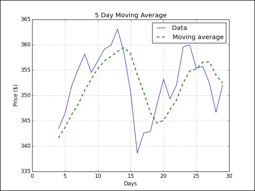
convolve(), we extracted the data in the center of sizeN. The following code makes an array of time values and plots withmatplotlibthat we will cover in a later chapter:c = np.loadtxt('data.csv', delimiter=',', usecols=(6,), unpack=True) sma = np.convolve(weights, c)[N-1:-N+1] t = np.arange(N - 1, len(c)) plt.plot(t, c[N-1:], lw=1.0, label="Data") plt.plot(t, sma, '--', lw=2.0, label="Moving average") plt.title("5 Day Moving Average") plt.xlabel("Days") plt.ylabel("Price ($)") plt.grid() plt.legend() plt.show()In the following chart, the smooth dashed line is the 5 day SMA and the jagged thin line is the close price:
We computed the SMA for the close stock price. It turns out that the SMA is just a signal processing technique—a convolution with weights 1/N, where N is the size of the moving average window. We learned that the ones() function can create an array with ones and the convolve() function calculates the convolution of a dataset with specified weights (see sma.py):
from __future__ import print_function
import numpy as np
import matplotlib.pyplot as plt

N = 5

weights = np.ones(N) / N
print("Weights", weights)

c = np.loadtxt('data.csv', delimiter=',', usecols=(6,), unpack=True)
sma = np.convolve(weights, c)[N-1:-N+1]
t = np.arange(N - 1, len(c))
plt.plot(t, c[N-1:], lw=1.0, label="Data")
plt.plot(t, sma, '--', lw=2.0, label="Moving average")
plt.title("5 Day Moving Average")
plt.xlabel("Days")
plt.ylabel("Price ($)")
plt.grid()
plt.legend()
plt.show()