
For this section, we will use two sample datasets, containing end-of-day price data. The first company is BHP Billiton (BHP), which is active in mining of petroleum, metals, and diamonds. The second is Vale (VALE), which is also a metals and mining company. So, there is some overlap of activity, albeit not 100 percent. For evaluating correlated pairs, follow these steps:
- First, load the data, specifically the close price of the two securities, from the CSV files in the example code directory of this chapter and calculate the returns. If you don't remember how to do it, look at the examples in Chapter 3, Getting Familiar with Commonly Used Functions.
- Covariance tells us how two variables vary together; which is nothing more than unnormalized correlation (see https://www.khanacademy.org/math/probability/regression/regression-correlation/v/covariance-and-the-regression-line):

Compute the covariance matrix from the returns with the
cov()function (it's not strictly necessary to do this, but it will allow us to demonstrate a few matrix operations):covariance = np.cov(bhp_returns, vale_returns) print("Covariance", covariance)The covariance matrix is as follows:
Covariance [[ 0.00028179 0.00019766] [ 0.00019766 0.00030123]]
- View the values on the diagonal with the
diagonal()method:print("Covariance diagonal", covariance.diagonal())The diagonal values of the covariance matrix are as follows:
Covariance diagonal [ 0.00028179 0.00030123]Notice that the values on the diagonal are not equal to each other. This is different from the correlation matrix.
- Compute the trace, the sum of the diagonal values, with the
trace()method:print("Covariance trace", covariance.trace())The trace values of the covariance matrix are as follows:
Covariance trace 0.00058302354992 - The correlation of two vectors is defined as the covariance, divided by the product of the respective standard deviations of the vectors. The equation for vectors
aandbis as follows:print(covariance/ (bhp_returns.std() * vale_returns.std()))
The correlation matrix is as follows:
[[ 1.00173366 0.70264666] [ 0.70264666 1.0708476 ]]
- We will measure the correlation of our pair with the correlation coefficient. The correlation coefficient takes values between
-1and1. The correlation of a set of values with itself is1by definition. This would be the ideal value; however, we will also be happy with a slightly lower value. Calculate the correlation coefficient (or, more accurately, the correlation matrix) with thecorrcoef()function:print("Correlation coefficient", np.corrcoef(bhp_returns, vale_returns))The coefficients are as follows:
[[ 1. 0.67841747] [ 0.67841747 1. ]]
The values on the diagonal are just the correlations of the BHP and VALE with themselves and are, therefore, equal to 1. In all likelihood, no real calculation takes place. The other two values are equal to each other since correlation is symmetrical, meaning that the correlation of BHP with VALE is equal to the correlation of VALE with BHP. It seems that here the correlation is not that strong.
- Another important point is whether the two stocks under consideration are in sync or not. Two stocks are considered out of sync if their difference is two standard deviations from the mean of the differences.
If they are out of sync, we could initiate a trade, hoping that they will eventually get back in sync again. Compute the difference between the close prices of the two securities to check the synchronization:
difference = bhp - vale
Check whether the last difference in price is out of sync; see the following code:
avg = np.mean(difference) dev = np.std(difference) print("Out of sync", np.abs(difference[-1] – avg) > 2 * dev)Unfortunately, we cannot trade yet:
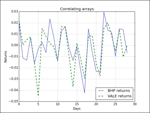
Out of sync False - Plotting requires
matplotlib; this will be discussed in Chapter 9, Plotting with matplotlib. Plotting can be done as follows:t = np.arange(len(bhp_returns)) plt.plot(t, bhp_returns, lw=1, label='BHP returns') plt.plot(t, vale_returns, '--', lw=2, label='VALE returns') plt.title('Correlating arrays') plt.xlabel('Days') plt.ylabel('Returns') plt.grid() plt.legend(loc='best') plt.show()The resulting plot is shown here:
We analyzed the relation of the closing stock prices of BHP and VALE. To be precise, we calculated the correlation of their stock returns. We achieved this with the corrcoef() function. Furthermore, we saw how to compute the covariance matrix from which the correlation can be derived. As a bonus, we demonstrated the diagonal() and trace() methods that give us the diagonal values and the trace of a matrix, respectively. For the source code, see the correlation.py file in this book's code bundle:
from __future__ import print_function
import numpy as np
import matplotlib.pyplot as plt
bhp = np.loadtxt('BHP.csv', delimiter=',', usecols=(6,), unpack=True)
bhp_returns = np.diff(bhp) / bhp[ : -1]
vale = np.loadtxt('VALE.csv', delimiter=',', usecols=(6,), unpack=True)
vale_returns = np.diff(vale) / vale[ : -1]
covariance = np.cov(bhp_returns, vale_returns)
print("Covariance", covariance)
print("Covariance diagonal", covariance.diagonal())
print("Covariance trace", covariance.trace())
print(covariance/ (bhp_returns.std() * vale_returns.std()))
print("Correlation coefficient", np.corrcoef(bhp_returns, vale_returns))
difference = bhp - vale
avg = np.mean(difference)
dev = np.std(difference)
print("Out of sync", np.abs(difference[-1] - avg) > 2 * dev)
t = np.arange(len(bhp_returns))
plt.plot(t, bhp_returns, lw=1, label='BHP returns')
plt.plot(t, vale_returns, '--', lw=2, label='VALE returns')
plt.title('Correlating arrays')

plt.xlabel('Days')
plt.ylabel('Returns')
plt.grid()
plt.legend(loc='best')
plt.show()