
CHAPTER 12
Capital Modeling
In this chapter, we explore the various methods for the calculation of operational risk capital and the challenges faced in adopting the Advanced Measurement Approach. New replacement methods are also considered, as these are scheduled for adoption in coming years. Different capital modeling methods are discussed and compared, and the use and importance of correlation and insurance offsets are considered. Finally, the disclosure requirements are introduced.
While banks are required to hold capital if they are subject to Basel II requirements, fintechs do not have this requirement. Fintechs rely on sponsor banks for the provision of much of their banking services, and those sponsor banks are subject to capital requirements in accordance with their national regulators.
OPERATIONAL RISK CAPITAL
Firms that are required to, or that choose to, calculate operational risk capital can select from several methods.
Basel II originally provided three main approaches to calculating operational risk capital: the Basic Indicator Approach, the Standardized Approach, and the Advanced Measurement Approach (AMA) (see Figure 12.1). These three methods will be considered first as they are still in place at the time of writing and were affirmed in 2019.1 However, future simplification of the calculation is scheduled for implementation soon and those new approaches are considered later in this chapter.
If an AMA is being used, then the calculation will draw on the underlying elements, as is illustrated in Figure 12.2. If a simpler approach is being used, then the underlying elements need not feed into the model.

FIGURE 12.1 The Three Basel II Operational Risk Capital Methods
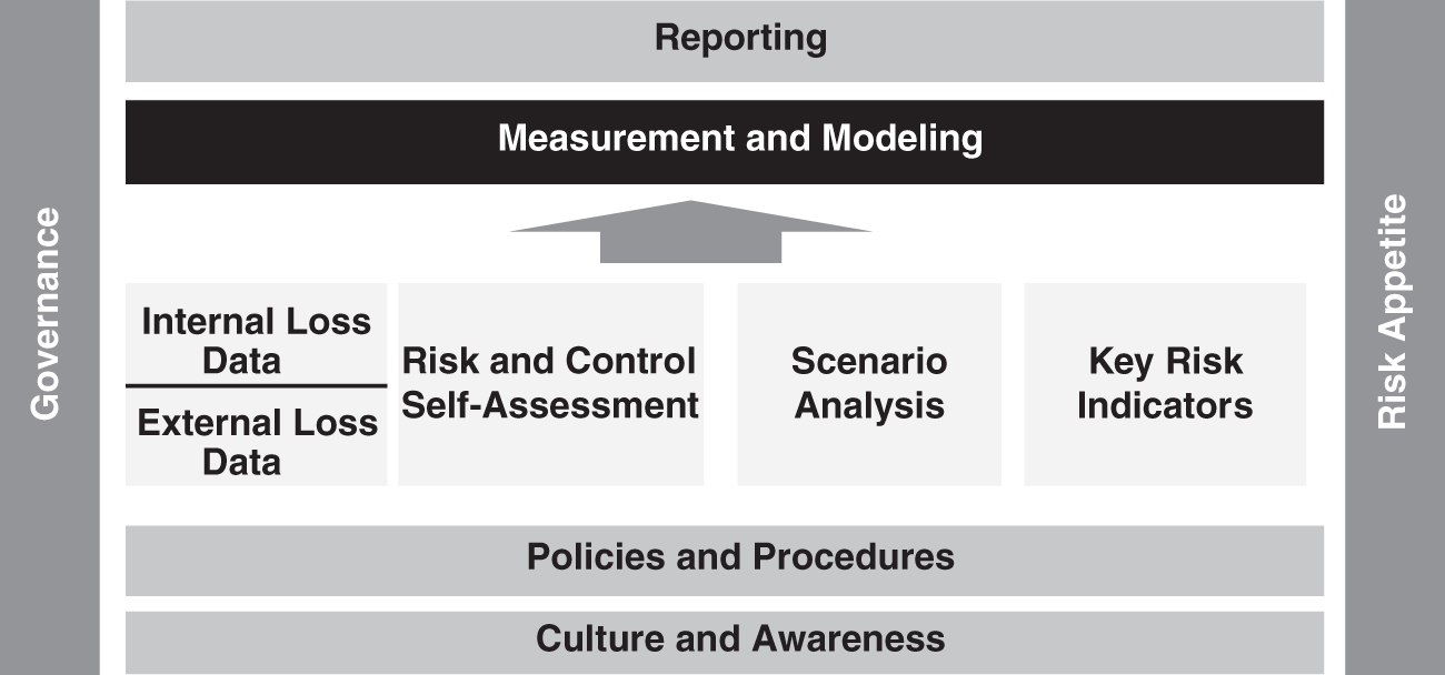
FIGURE 12.2 The Role of Capital Modeling in the Operational Risk Framework
Under the Basel II rules, banks are encouraged to move toward the more sophisticated approaches as they develop their operational risk management tools. Basel II expected international active banks to select either the Standardized or Advanced Measurement Approaches. Many national regulators also brought in mandatory requirements that forced large financial institutions to adopt the Advanced Measurement Approach for operational risk if they wished to be approved for Basel II overall.
Recent analysis of the effectiveness of the advanced methods has led to a change in direction, as is discussed later.
BASIC INDICATOR APPROACH
Under the Basic Indicator Approach (BIA), the capital calculation is arrived at through a simple calculation of the average gross revenue for the past three years, multiplied by 15 percent. The 2019 Bank of International Settlements (BIS) guidance outlines the approach as follows:
Banks using the Basic Indicator Approach must hold capital for operational risk equal to the average over the previous three years of a fixed percentage (denoted alpha) of positive annual gross income. Figures for any year in which annual gross income is negative or zero should be excluded from both the numerator and denominator when calculating the average. The charge may be expressed as follows:2
where:
| KBIA | = | the capital charge under the Basic Indicator Approach |
| GI | = | annual gross income, where positive, over the previous three years |
| N | = | the number of the previous three years for which gross income is positive |
| α | = | 15 percent, which is set by the Committee, relating the industry-wide level of required capital to the industry-wide level of the indicator |
| Gross income is defined as net interest income plus net noninterest income.3 | ||
Firms that used this approach were still encouraged to adopt all of the risk management elements that are outlined in the “Sound Practices”4 document. Therefore, even though loss data, RCSA, scenario analysis, and business environment internal control factors (BEICF) are not needed for the capital calculation, they are needed as part of the operational risk framework to ensure that the firm can adequately identify, assess, monitor, and mitigate operational risk as required in the “Sound Practices” document.
If a bank has negative or zero income for any of the three years, then BIA instructs them to remove those years from both the numerator and denominator when calculation the average revenue.
The Basic Indicator Approach to capital is certainly simple to adopt but does little to reflect the operational risk in a firm, as it uses only revenue as a driver. A firm that has very strong controls will have the same operational risk requirements as a firm with very poor controls if they have had the same average revenue over the past three years.
Furthermore, a firm will enjoy much lower operational risk capital requirements in years when it is producing lower revenue, even if its controls have not changed at all.
STANDARDIZED APPROACH
The Standardized Approach (TSA) originally provided under Basel II is similar to the Basic Indicator Approach, except that different business lines have different multipliers. The Standardized Approach attempts to capture operational risk factors that are missing in the Basic Indicator Approach by assuming that different types of business activities carry different levels of operational risk. Sales and trading is riskier than retail brokerage, for example. The 2019 BIS guidance puts it thus:
Within each business line, gross income is a broad indicator that serves as a proxy for the scale of business operations and thus the likely scale of operational risk exposure within each of these business lines.5
As a result, although the calculation method is the same, the multiplier used varies according to the business line. This will result in several separate calculations that are then brought together for the total operational risk capital.
The total capital requirement is calculated as the three-year average of the simple summation of the regulatory capital requirements across each of the business lines in each year. In any given year, negative capital charges (resulting from negative gross income) in any business line may offset positive capital charges in other business lines without limit.
However, where the aggregate capital charge across all business lines within a given year is negative, then the input to the numerator for that year will be zero. The total capital charge may be expressed as:

where:
| KTSA | = | the capital charge under the standardized approach |
| GI 1–8 | = | annual gross income in a given year, as defined above in the basic indicator approach, for each of the eight business lines |
| β 1–8 | = | a fixed percentage, set by the Committee, relating the level of required capital to the level of the gross income for each of the eight business lines. The values of the betas are detailed below.6 |
| Business Lines | Beta Factors |
|---|---|
| Corporate finance (β1) | 18% |
| Trading and sales (β2) | 18% |
| Retail banking (β3) | 12% |
| Commercial banking (β4) | 15% |
| Payment and settlement (β5) | 18% |
| Agency services (β6) | 15% |
| Asset management (β7) | 12% |
| Retail brokerage (β8) | 12% |
The TSA calculation of operational risk capital is no more difficult than the BIA, but it does have significantly more steps, as a calculation must be made for all business lines in order to produce the final capital result.
In the following example, Beta Bank has only three lines of business and is using the TSA calculation method for its operational risk capital.
If there is negative or zero income during one of the three prior years, TSA takes a different treatment approach than that used in the BIA. In the BIA, any years that have negative or zero income are removed from both the denominator and the numerator. However, under TSA:
In any given year, negative capital charges (resulting from negative gross income) in any business line may offset positive capital charges in other business lines without limit. However, where the aggregate capital charge across all business lines within a given year is negative, then the input to the numerator for that year will be zero.7
Note that the denominator in TSA is set at 3.
Alternative Standardized Approach
Basel II allowed a national regulator to permit a bank to use an Alternative Standardized Approach (ASA) provided “the bank is able to satisfy its supervisor that this alternative approach provides an improved basis by, for example, avoiding double counting of risks.”8
Under the ASA, the operational risk capital charge/methodology is the same as for the Standardized Approach except for two business lines—retail banking and commercial banking. For these business lines, loans and advances—multiplied by a fixed factor “m”—replaces gross income as the exposure indicator …
The ASA operational risk capital requirement for retail banking (with the same basic formula for commercial banking) can be expressed as:
where:
| KRB | = | the capital charge for the retail banking business line |
| β RB | = | the beta for the retail banking business line |
| LA RB | = | total outstanding retail loans and advances (non-risk-weighted and gross of provisions), averaged over the past three years |
| m | = | 0.035 |
| For the purposes of the ASA, total loans and advances in the retail banking business line consist of the total drawn amounts in the following credit portfolios: retail, SMEs treated as retail, and purchased retail receivables. For commercial banking, total loans and advances consist of the drawn amounts in the following credit portfolios: corporate, sovereign, bank, specialized lending, SMEs treated as corporate and purchased corporate receivables. The book value of securities held in the banking book should also be included. | ||
| Under the ASA, banks may aggregate retail and commercial banking (if they wish to) using a beta of 15 percent. | ||
| Similarly, those banks that are unable to disaggregate their gross income into the other six business lines can aggregate the total gross income for these six business lines using a beta of 18 percent, with negative gross income treated as described in paragraphs OPE25.3 and OPE25.4. | ||
| As under the Standardized Approach, the total capital requirement for the ASA is calculated as the simple summation of the regulatory capital charges across each of the eight business lines.9 | ||
Future of the Basic and Standardized Approaches
The BIA and TSA methodologies can produce an unanticipated result as is demonstrated in the following example.
This was likely not the intent of the Basel Committee, and they recognized that making allowances for negative income might produce an inappropriate result.
If negative gross income distorts a bank's Pillar 1 capital requirement … supervisors will consider appropriate supervisory action under Pillar 2.10
Therefore, if the use of negative income offsets produces an unpalatable or inappropriate result, then a bank may see its regulators adding on capital under the Pillar 2 requirements of Basel II. As discussed in Chapter 2, Pillar 2 provides a mechanism for additional capital requirements to cover any material risks that have not been effectively captured in Pillar 1.
The revised Standardized Approach that is discussed later in this chapter also addresses this issue.
ADVANCED MEASUREMENT APPROACH
The Advanced Measurement Approach (AMA) allowed a bank to design its own model for calculating operational risk capital. The Basel Committee recognized that they were allowing significant flexibility for the design of the AMA capital model and established prerequisites for its use as follows:
General Standards for Using the AMA
In order to qualify for use of the AMA a bank must satisfy its supervisor that, at a minimum:
Its board of directors and senior management, as appropriate, are actively involved in the oversight of the operational risk management framework;
It has an operational risk management system that is conceptually sound and is implemented with integrity; and
It has sufficient resources in the use of the approach in the major business lines as well as the control and audit areas.11
In addition, a bank's regulator must monitor the proposed AMA to ensure that it is appropriate before it can be relied upon for the calculation of capital:
A bank's AMA will be subject to a period of initial monitoring by its supervisor before it can be used for regulatory purposes. This period will allow the supervisor to determine whether the approach is credible and appropriate.12
The four elements of the framework—internal loss data, external loss data, scenario analysis, and business environment internal control factors—must be included in the model.
As discussed below, a bank's internal measurement system must reasonably estimate unexpected losses based on the combined use of internal and relevant external loss data, scenario analysis and bank-specific business environment and internal control factors.13
The final prerequisite is that there must be an appropriate method for allocating the capital to the businesses to incent good behavior.
The bank's measurement system must also be capable of supporting an allocation of economic capital for operational risk across business lines in a manner that creates incentives to improve business line operational risk management.14
Quantitative Requirements of an AMA Model
Once the prerequisites have been met, there are several quantitative requirements that must be adhered to for an AMA model.
One Year and 99.9 Percent
The first requirement is that the model must hold capital for a one-year horizon at 99.9 percent confidence level. In other words, the capital held must be sufficient to cover all operational risk losses in one year with a certainty of 99.9 percent.
This is the equivalent of asking for a bank to hold operational risk capital that will protect it from a 1-in-1,000-year fat-tail event.
Given the continuing evolution of analytical approaches for operational risk, the Committee is not specifying the approach or distributional assumptions used to generate the operational risk measure for regulatory capital purposes. However, a bank must be able to demonstrate that its approach captures potentially severe “tail” loss events. Whatever approach is used, a bank must demonstrate that its operational risk measure meets a soundness standard comparable to that of the internal ratings-based approach for credit risk (i.e., comparable to a one year holding period and a 99.9th percentile confidence interval).15
Model Governance
The second requirement is that the model must be subject to full model governance.
In the development of operational risk measurement and management systems, banks must have and maintain rigorous procedures for operational risk model development and independent model validation.16
Model Design
The third requirement concerns the design of the AMA model and several stipulations that must be met.
The first stipulation is that the model must represent the operational risk framework as outlined in Basel II and supporting guidance.
Any internal operational risk measurement system must be consistent with the scope of operational risk defined in OPE10.1 and the loss event types defined in Table 1.17
In effect, this means that calculations should be made for all seven risk categories. Some firms calculate capital at the top of the firm and then allocate operational risk capital down into the business lines. Others calculate capital at the business line. Table 12.1 shows a matrix for capital calculations using the Basel business lines. However, a firm might have different headings in the first column to better represent their own business line structure.
The second stipulation is that the model must capture all expected and unexpected losses and may only exclude expected losses under certain strict criteria.
Supervisors will require the bank to calculate its regulatory capital requirement as the sum of expected loss (EL) and unexpected loss (UL), unless the bank can demonstrate that it is adequately capturing EL in its internal business practices. That is, to base the minimum regulatory capital requirement on UL alone, the bank must be able to demonstrate to the satisfaction of its national supervisor that it has measured and accounted for its EL exposure.18
The third stipulation is that the model must provide sufficient detail and granularity to ensure that fat-tail events are captured.
TABLE 12.1 Example Capital Calculation Matrix
| Internal Fraud | External Fraud | Clients, Products, and Business Practices | Execution, Delivery, and Process Management | Employment Practices and Workplace Safety | Damage to Physical Assets | Business Disruption and System Failures | |
|---|---|---|---|---|---|---|---|
| Corporate Finance | |||||||
| Trading and Sales | |||||||
| Retail Banking | |||||||
| Commercial Banking | |||||||
| Payment and Settlement | |||||||
| Agency and Custody | |||||||
| Retail Brokerage | |||||||
| Asset Management |
A bank's risk measurement system must be sufficiently “granular” to capture the major drivers of operational risk affecting the shape of the tail of the loss estimates.19
The fourth stipulation is that the bank must sum all calculated cells or defend any correlation assumptions that are made in its AMA model.
Risk measures for different operational risk estimates must be added for purposes of calculating the regulatory minimum capital requirement. However, the bank may be permitted to use internally determined correlations in operational risk losses across individual operational risk estimates, provided it can demonstrate to the satisfaction of the national supervisor that its systems for determining correlations are sound, implemented with integrity, and take into account the uncertainty surrounding any such correlation estimates (particularly in periods of stress). The bank must validate its correlation assumptions using appropriate quantitative and qualitative techniques.20
The fifth stipulation simply reinforces the requirement that all four elements must be in the model.
Any operational risk measurement system must have certain key features to meet the supervisory soundness standard set out in this section. These elements must include the use of internal data, relevant external data, scenario analysis and factors reflecting the business environment and internal control systems.21
Finally, the bank must weight these four elements appropriately.
A bank needs to have a credible, transparent, well-documented and verifiable approach for weighting these fundamental elements in its overall operational risk measurement system.22
The Basel rules also provide many qualitative requirements that must be met in order for a bank to qualify for an AMA model for Basel II. Many of these have been discussed in prior chapters, for example the rules regarding the collection and use of loss data, the challenges of scenario analysis, and the use of BEICF from RCSA and KRI elements in the operational risk framework.
While the four elements must be considered in the capital calculation methodology, many banks use some of these elements to allocate capital, to stress-test their models, or to adjust their models rather than using them to provide direct inputs into the capital calculation. Regulators have accepted many different models for AMA and the modeling of operational risk capital is developing rapidly as different approaches are tried and tested by the banking industry.
Many firms, however, spent many years wrestling with building and receiving approval for their AMA models, and the most recent guidance has removed the AMA option. At the time of this writing, this sunsetting of the AMA model was to occur in 2023, but that date has been moved out several times.
As a result, the AMA is still currently a viable approach to calculating operational risk capital under existing Basel II rules and so we will consider some of the modeling options that are available below.
Loss Distribution Approach to Modeling Operational Risk Capital
A loss distribution approach (LDA) model relies on internal losses as the mainstay of its design. A simple LDA model uses only internal losses as direct inputs into the model and uses the remaining three elements for stressing or allocation purposes.
A bank must have at least three years of loss data to put into its AMA model, regardless of design, as the data may be rich enough to form the basis of a capital model.
Internally generated operational risk measures used for regulatory capital purposes must be based on a minimum five-year observation period of internal loss data, whether the internal loss data is used directly to build the loss measure or to validate it. When the bank first moves to the AMA, a three-year historical data window is acceptable.23
Despite this stipulation, regulators leaned toward requiring all available data to be included, even beyond the five-year requirement. In their 2011 AMA Guidelines, the Basel Committee noted:
The Basel II Framework requires banks to base their internally generated operational risk measures on a minimum historical observation period of five years (three years when an institution first moves to an AMA). For certain ORCs with low frequency of events, an observation period greater than five years may be necessary to collect sufficient data to generate reliable operational risk measures and ensure that all material losses are included in the calculation dataset.24
The advantage of a loss distribution approach is that the model is based on real historical data that is relevant to the firm.
The disadvantage of a loss distribution approach is that the period of data collection is likely to be relatively short, and so may not have captured the fat-tail events that the capital calculation is supposed to protect the firm from. It certainly will not contain 1,000 years of data, and yet the model is supposed to provide a 99.9 percent confidence level. Some firms also find that they have insufficient loss data on which to build a model even if they have more than five years of data.
In addition, historical data does not necessarily reflect the future. The firm may have changed its products, processes, and controls.
Although there is a wide range of AMA modeling practices, even within the LDA approach, there are some standard methods that are worthy of discussion.
Step 1: Modeling Frequency
In order to develop a model of expected operational risk losses, the first step is to determine the likely number of events per year. This is the frequency of events.
The most popular distribution selection for modeling frequency is the Poisson distribution. This allows for a fairly simple approach to modeling frequency. In a Poisson distribution, there is only a single parameter (λ), which represents the average number of events in a given year. Both the mean and the variance are represented by this single parameter in a Poisson distribution. In more complex cases, a negative binomial distribution may be used, which allows for different values for the mean and variance.
The Poisson distribution works well for a situation where there is a whole number of events and where the probability in one time period is the same as in another time period. The Poisson distribution is built from the use of the average number of events using the following formula.
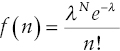
where:
| n | = | 0, 1, 2, … . |
| λ | = | average number of events in a year |
In an LDA model, λ can be obtained simply by observing the number of events per year in the internal loss data history and calculating the average.
The Poisson distribution that is derived from this approach represents the probability of a certain number of events occurring in a single year. As can be seen in Figure 12.3, lower lambdas produce more skewed and leptokurtic25 annual loss distributions than higher lambdas.
Step 2: Modeling Severity
The next step in modeling expected operational risk losses is to determine the likely size of an event given the fact that an event has occurred. This is the severity of an event.
Unlike frequency, severity need not be an integer but can fall anywhere along a continuum. When a loss occurs, it might be $1.50, or it might be $133,892.25 or any other value. The severity distribution establishes the probability of an event occurring over a wide range of values, from zero to very, very large losses.
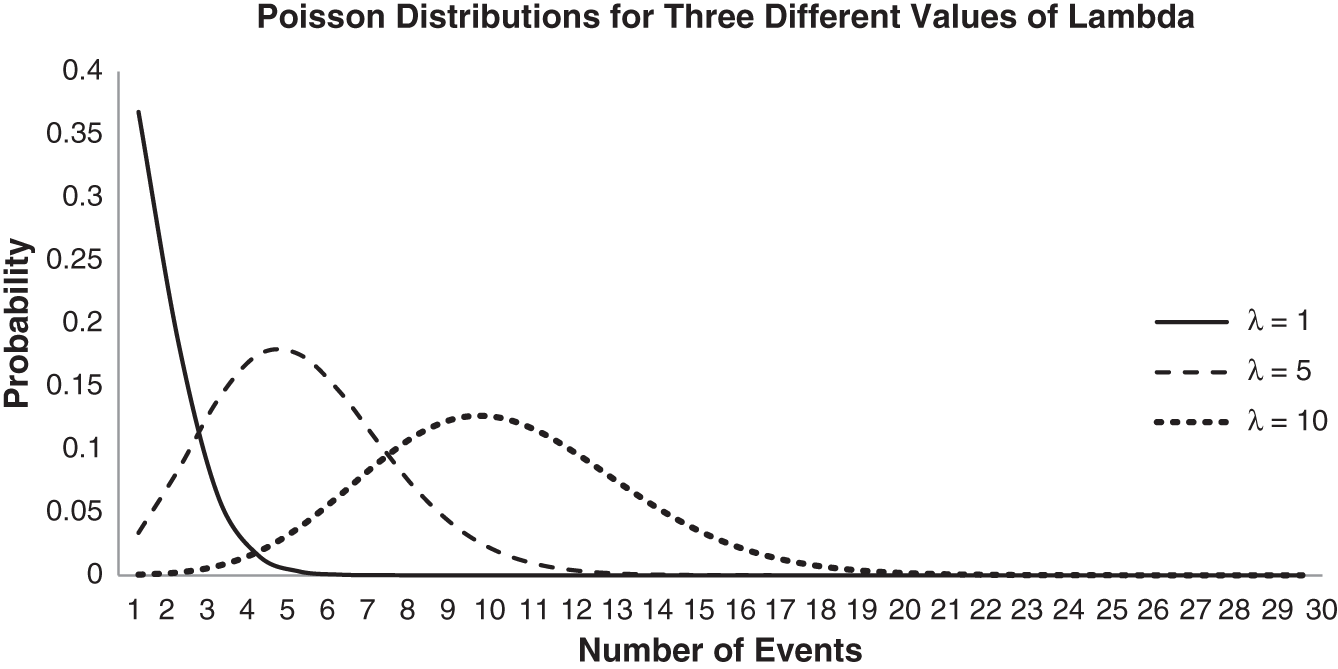
FIGURE 12.3 Comparing Three Different Poisson Distributions
The most common and least complex approach to modeling severity is to use a lognormal distribution, although low-frequency losses may fit better to other options such as Generalized Gamma, Transformed Beta, Generalized Pareto, or Weibull. Regulators take a keen interest in how well the selected distribution demonstrates “goodness of fit”—or in other words, how certain you are that the sample comes from the population with the claimed distribution. When selecting which approach to use, the AMA guidelines also provide the following guidance (emphasis added):
The selection of probability distributions should be consistent with all elements of the AMA model. In addition to statistical goodness of fit, Dutta and Perry (2007) have proposed the following criteria for assessing a model's suitability:
- realistic (e.g., it generates a loss distribution with a realistic capital requirements estimate, without the need to implement “corrective adjustments” such as caps),
- well specified (e.g., the characteristics of the fitted data are similar to the loss data and logically consistent),
- flexible (e.g., the method is able to reasonably accommodate a wide variety of empirical data) and
- simple (e.g., it is easy to implement and it is easy to generate random numbers for the purpose of loss simulation).
The process of selecting the probability distribution should be well-documented, verifiable and lead to a clear and consistent choice. To this end, a bank should generally adhere to the following:
- Exploratory Data Analysis (EDA) for each ORC to better understand the statistical profile of the data and select the most appropriate distribution;
- Appropriate techniques for the estimation of the distributional parameters; and
- Appropriate diagnostic tools for evaluating the quality of the fit of the distributions to the data, giving preference to those most sensitive to the tail.26
Whichever distribution is selected, the probability density function for severity will have a fat tail, that is, very large events (beyond three standard deviations of the mean) are more likely to occur than in a normal distribution. It will also be skewed to the right, as can be seen in the example in Figure 12.4.
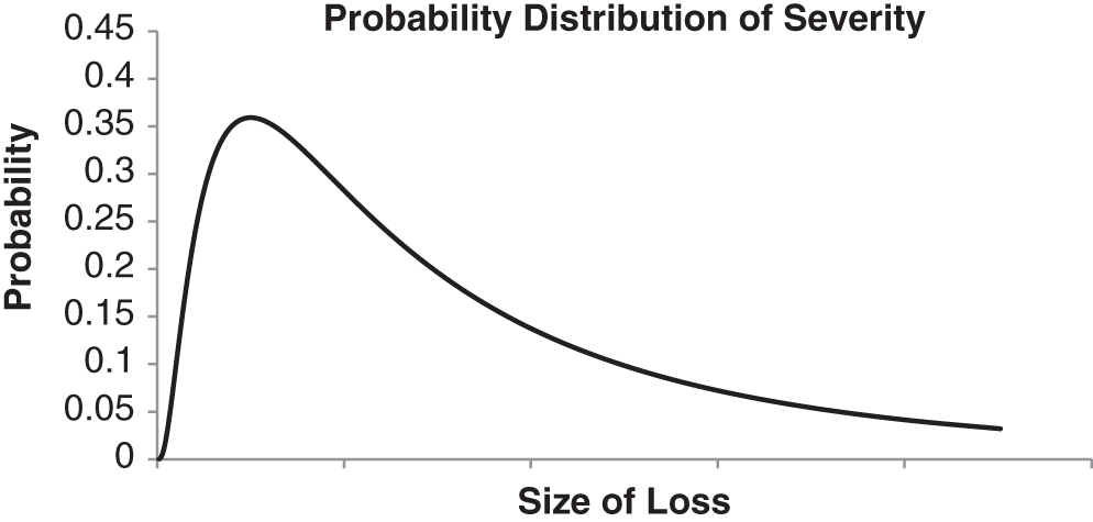
FIGURE 12.4 The Severity Probability Distribution
Step 3: Monte Carlo Simulation
Once the frequency and severity distributions have been established, the next step is to use these distributions to generate many more data points in order to better estimate the capital needed to ensure with 99.9 percent certainty that likely losses for the next year are covered by appropriate capital.
Monte Carlo simulation provides a method by which frequency and severity distributions can be combined to produce many more data points that have the same characteristics as the observed data points. Excel can handle this process using built-in functionality, but often much more powerful statistical modeling tools are used.
First, a data point is selected from the frequency distribution. This gives us the number of events that are predicted to occur in year one. Values nearer the mean of the frequency distribution will be selected more often than values far from the mean. In this example, let us say that the number 50 is selected. Therefore, in year one the model assumes there were 50 events.
Next, the size of each of those 50 events is selected from the severity distribution. Again, values with a higher probability in the severity distribution will be selected more often than values with a lower probability. This will produce 50 losses for year one.
The value of all 50 losses is then added together to give the total value of losses for year one.
This process is repeated for year two, and then over and over again, a million times, thus giving the modeler many additional years of representative data. The data is then placed in size order, the largest total year loss, to the smallest total year loss.

FIGURE 12.5 Using Monte Carlo Simulation
Finding the 99.9 percent confidence level is simply a case of selecting the one thousandth item in the ordered list. That value represents, with 99.9 percent certainty, the maximum loss that will be experienced in a single year.
This process is represented in Figure 12.5.
Correlation
Once all of the cells of the operational risk capital matrix have been populated, with a calculated capital amount for each risk category, and possibly also for every business line, then all of the cells must be simply added together to produce the total capital required. However, firms can take advantage of correlation assumptions between cells if these assumptions can be defended.
Risk measures for different operational risk estimates must be added for purposes of calculating the regulatory minimum capital requirement. However, the bank may be permitted to use internally determined correlations in operational risk losses across individual operational risk estimates, provided it can demonstrate to the satisfaction of the national supervisor that its systems for determining correlations are sound, implemented with integrity, and take into account the uncertainty surrounding any such correlation estimates (particularly in periods of stress). The bank must validate its correlation assumptions using appropriate quantitative and qualitative techniques.27
Some firms have found the ORX data useful for this purpose. ORX data contains loss data for all risk categories for all firms that are consortium members. If a correlation matrix can be established for that large pool of data it might be possible to use those same assumptions for the internal AMA model of a member firm. With no correlation assumptions, the additive nature of the model can produce very high capital results. As a result there is an enormous amount of work (internally and with consulting firms) currently under way in the industry, as firms attempt to better support correlation assumptions for use in operational risk capital modeling.
Scenario Analysis Approach to Modeling Operational Risk Capital
A pure scenario analysis approach to modeling uses only scenario analysis data in the model. The other three required elements are used for stress testing, validation, or allocation.
Scenario analysis data is designed to identify fat-tail events, and therefore may provide rich data for the calculation of appropriate operational risk capital.
One of the advantages of a scenario analysis approach is that the data reflects the future as it is captured in a process that is designed to consider “what if” scenarios. In contrast, an LDA approach is only considering the past.
One of the major disadvantages of a scenario analysis approach is that the data is highly subjective, as it has probably been gathered in an interview or workshop estimation exercise. Also, scenario analysis produces only a few data points and so complex techniques have to be applied to model the data into a full distribution.
While the same methods for frequency and severity distributions and Monte Carlo simulations might be used as in the LDA approach described earlier, the lack of data in scenario analysis output can make the fitting of distributions particularly troublesome. A small change in assumptions can lead to very different results, and therefore the defense of all assumptions must be particularly robust in a scenario analysis approach.
The data for use in the model may look similar to the output example in Chapter 11 and shown again in Table 12.2, or it might be a simple series of maximum loss amounts per risk category, or per scenario.
There are many possible outputs from the many different scenario approaches in use. Whatever scenario analysis method is used, there will likely be a paucity of data points, and so a pure scenario analysis approach can be difficult to defend. Indeed, although some scenario-based models may have been approved in Europe, they are generally frowned upon by the regulators in the United States.
Certainly, the more reliance there is on scenario analysis, the more robust the scenario analysis program must be.
TABLE 12.2 Sample Scenario Analysis Output
| Frequency/Severity Buckets | Total Annual Frequency | Max Single Loss | ||||||
|---|---|---|---|---|---|---|---|---|
| Risk Category | $1 to $5m | $5 to $10m | $10 to $20m | $20 to $50m | $50 to $100m | > $100m | ||
| Clients, Products, and Business Practices | 5.0(A) | 3.0 | 1.0 | 0.5 | 0.2 | 0.1(B) | 9.8(C) | $600m(D) |
| Execution, Delivery, and Process Management | 10.0 | 5.0 | 2.0 | 0.5 | 0.2 | 0.1 | 17.8 | $150m |
| External Fraud | 1.0 | 0.5 | 0.2 | 0.1 | – | – | 1.8 | $45m |
| Internal Fraud | 1.0 | 0.5 | 0.1 | 0.1 | 0.1 | 0.1 | 1.9 | $1,000m |
| Damage to Physical Assets | 3.0 | 1.0 | 1.0 | 0.5 | 0.2 | 0.1 | 5.8 | $100m |
| Employee Practices and Workplace Safety | 5.0 | 3.0 | 2.0 | 1.0 | 0.5 | – | 22.5 | $75m |
| Business Disruption and Systems Failures | 6.0 | 4.0 | 2.0 | 1.0 | – (E) | – | 13 | $40m |
There may well be cells in the model that rely on a pure scenario analysis model simply because there is little or no loss data available in that cell. It is acceptable to have different modeling techniques in different cells of the model as long as the differences are justified.
Hybrid Approach to Modeling Operational Risk Capital
Many firms have some version of a hybrid approach. In a hybrid approach, the loss data and scenario analysis output are both used to calculate appropriate operational risk capital.
Some firms combine the LDA and scenario analysis approaches by stitching together two distributions, for example, by using LDA for the left end of the distribution, or the expected losses, and scenario analysis for the right end of the distribution, or the fat-tail and unexpected losses. Some firms develop a LDA model and then use scenario analysis to stress the model to produce a more appropriate distribution. Some firms add their scenario analysis data points into their loss data and develop their frequency and severity distributions from the combined data pool.
In a hybrid approach, the advantages and disadvantages of both approaches are present.
INSURANCE
Businesses will often argue that they are not exposed to operational risk in certain risk categories or scenarios because they carry insurance against just such risks arising. However, insurance payments can be slow and contentious and therefore Basel II does not allow for insurance to be used to reduce the gross amount of the loss, except under very narrow circumstances.
Under the AMA, a bank will be allowed to recognize the risk-mitigating impact of insurance in the measures of operational risk used for regulatory minimum capital requirements, but only if specific, fairly onerous, criteria are met.
The recognition of insurance mitigation is limited to 20 percent of the total operational risk capital charge calculated under the AMA.
The qualifying criteria are as follows:
A bank's ability to take advantage of such risk mitigation will depend on compliance with the following criteria:
The insurance provider has a minimum claims paying ability rating of A (or equivalent).
- The insurance policy must have an initial term of no less than one year. For policies with a residual term of less than one year, the bank must make appropriate haircuts reflecting the declining residual term of the policy, up to a full 100% haircut for policies with a residual term of 90 days or less.
- The insurance policy has a minimum notice period for cancellation of 90 days.
- The insurance policy has no exclusions or limitations triggered by supervisory actions or, in the case of a failed bank, that preclude the bank, receiver or liquidator from recovering for damages suffered or expenses incurred by the bank, except in respect of events occurring after the initiation of receivership or liquidation proceedings in respect of the bank, provided that the insurance policy may exclude any fine, penalty, or punitive damages resulting from supervisory actions.
- The risk mitigation calculations must reflect the bank's insurance coverage in a manner that is transparent in its relationship to, and consistent with, the actual likelihood and impact of loss used in the bank's overall determination of its operational risk capital.
- The insurance is provided by a third-party entity. In the case of insurance through captives and affiliates, the exposure has to be laid off to an independent third-party entity, for example through re-insurance, that meets the eligibility criteria.
- The framework for recognizing insurance is well reasoned and documented.
- The bank discloses a description of its use of insurance for the purpose of mitigating operational risk.
A bank's methodology for recognizing insurance under the AMA also needs to capture the following elements through appropriate discounts or haircuts in the amount of insurance recognition:
- The residual term of a policy, where less than one year, as noted above;
- A policy's cancellation terms, where less than one year; and
- The uncertainty of payment as well as mismatches in coverage of insurance policies.28
Operational risk capital may run into many billions of dollars, so it is certainly worth pursuing a 20 percent reduction in that amount, and many firms have explored how best to take advantage of this opportunity. At the same time, many insurance companies are looking to produce insurance products that can meet the many criteria required. In the disclosure examples later in this chapter, firms have outlined their approach to the use of insurance to lower their operational risk capital requirements.
FUTURE OF CAPITAL REQUIREMENTS: BASEL III
Basel II regulators around the world have accepted all types of modeling approaches in AMA banks to date and the Basel Committee commented in their 2011 AMA Guidelines document on the wide range of practice that they had observed. In developing the Basel III capital requirements for operational risk, the Bank of International Settlements (BIS) noted that the AMA had not provided sufficient capital coverage for the economic crisis that occurred in 2008.
BIS's choice of values for alpha and beta in BIA and TSA were made with little supporting data, and the Basel Committee reviewed the assumptions that were made when those values were selected. This was always their intention and was clearly stated in Basel II.
The Committee intends to reconsider the calibration of the Basic Indicator and Standardized Approaches when more risk-sensitive data are available to carry out this recalibration. Any such recalibration would not be intended to affect significantly the overall calibration of the operational risk component of the Pillar 1 capital charge.29
This reconsideration occurred in 2011–2012, and it was generally expected that the alpha and beta values had not stood up to testing now that data was available on business line operational risk losses.
In addition to questions being raised about the alpha and beta values of the BIA and TSA, there have been concerns raised about the range of practice found in the implementation of AMA calculations. In Basel II, the Basel Committee stated:
Supervisors will review the capital requirement produced by the operational risk approach used by a bank (whether Basic Indicator Approach, Standardized Approach or AMA) for general credibility, especially in relation to a firm's peers. In the event that credibility is lacking, appropriate supervisory action under Pillar 2 will be considered.29
The review of the effectiveness of the operational risk capital approaches led eventually to the introduction of Basel III requirements for operational risk capital. This new approach was introduced in 2017 and required the sunsetting of the use of AMA, replacing it with a simplified Standardized Approach.
Therefore, while the industry continued to refine their AMA models, the rules have now changed and, at the time of this writing, the new approach must be adopted by January 2023.
Basel III Standardized Approach
In 2017, BCBS issued new guidance in “Finalizing Post-Crisis Reforms,” as follows:
The standardised approach for measuring minimum operational risk capital requirements replaces all existing approaches in the Basel II framework. That is, this standard replaces paragraphs 644 to 683 of the Basel II framework.
The standardised approach methodology is based on the following components:
- the Business Indicator (BI) which is a financial-statement-based proxy for operational risk;
- the Business Indicator Component (BIC), which is calculated by multiplying the BI by a set of regulatory determined marginal coefficients (αi); and
- the Internal Loss Multiplier (ILM), which is a scaling factor that is based on a bank's average historical losses and the BIC.30
The new Standardized Approach disallows the use of an internal model that is derived from the four elements that make up the AMA approach and instead relies only on the internal loss experience of the firm and its business lines. The use of the other elements—external loss data, scenario analysis, and business environment internal control factors—as direct inputs to the model is no longer permissible once the new requirements go into effect (2023 at the time of this writing). However, the guidance regarding the sound principles of operational risk management still stand and so those elements are still required for the purposes of demonstrating effective operational risk management.
The calculation of the new Standardized Approach is as follows:
where:
| OTC | = | operational risk capital |
| BIC | = | business indicator component |
| ILM | = | internal loss multiplier |
Banks that have a BI of €1 billion or less have a simplified requirement for capital and are required to hold capital that is equal to their business indicator component (BIC), with no adjustment for the internal loss multiplier (ILM). This allows smaller banks to avoid the strict requirements for internal loss data collection that are required for the inclusion of the ILM in the calculation.
The BIC is calculated from the business indicator.
The Business Indicator BI
The first building block of the new Standardized Approach is the business indicator (BI). As stated earlier, the BI is a financial-statement-based proxy for operational risk.
The BI comprises three components: the interest, leases, and dividend component (ILDC); the services component (SC); and the financial component (FC).
The BI is calculated as follows:
The three factors that make up the BI are derived as outlined below.
First, the ILDC is derived as follows:
where:
| II | = | Average interest income over the prior three years |
| IE | = | Average interest expense over the prior three years |
| IEA | = | Average interest-earning assets over the prior three years |
| DI | = | Average dividend interest over the prior three years |
Secondly, the services component (SC) is derived as follows:
where:
| OOI | = | Average other operating Income over the prior three years |
| OOE | = | Average other operating expense over the prior three years |
| FI | = | Average fee income over the prior three years |
| FE | = | Average fee expense over the prior three years |
Finally, the financial component (FC) is derived as follows:
where:
| Net PLTB | = | Average net P&L trading book over the prior three years |
| Net PLBB | = | Average net P&L banking book over the prior three years |
The definitions of what makes up each of these indicators is outlined in the annex of the latest Basel guidance, as shown in Table 12.3.
Business Indicator Component: BIC
The next step in the new Standardized Approach calculation is to derive the BIC from the BIs as follows:
To calculate the BIC, the BI is multiplied by the marginal coefficients (αi). The marginal coefficients increase with the size of the BI as shown in Table 1. For banks in the first bucket (i.e. with a BI less than or equal to €1bn) the BIC is equal to BI × 12%. The marginal increase in the BIC resulting from a one unit increase in the BI is 12% in bucket 1, 15% in bucket 2 and 18% in bucket 3. For example, given a BI = €35bn, the BIC = (1 × 12%) + (30 – 1) × 15% + (35 – 30) × 18% = €5.37bn.32
| Table 1 BI Ranges and Marginal Coefficients | ||
|---|---|---|
| Bucket | BI Range (in €bn) | BI Marginal Coefficients (αi) |
| 1 | ≤1 | 12% |
| 2 | 1 < BI ≤ 30 | 15% |
| 3 | > 30 | 18% |
TABLE 12.3 Definitions of the Business Indicator Component
| BI Component | P&L or Balance Sheet Items | Description | Typical Subitems |
|---|---|---|---|
| Interest, lease, and dividend | Interest income | Interest income from all financial assets and other interest income (includes interest income from financial and operating leases and profits from leased assets) |
|
| Interest expenses | Interest expenses from all financial liabilities and other interest expenses (includes interest expense from financial and operating leases, losses, depreciation, and impairment of operating leased assets) |
| |
| Interest-earning assets (balance sheet item) | Total gross outstanding loans, advances, interest bearing securities (including government bonds), and lease assets measured at the end of each financial year | ||
| Dividend income | Dividend income from investments in stocks and funds not consolidated in the bank's financial statements, including dividend income from nonconsolidated subsidiaries, associates and joint ventures. | ||
| Services | Fee and commission income | Income received from providing advice and services. Includes income received by the bank as an outsourcer of financial services. | Fee and commission income from:
|
| Fee and commission expenses | Services | Fee and commission expenses from:
| |
| Other operating income | Income from ordinary banking operations not included in other BI items but of similar nature (income from operating leases should be excluded) |
| |
| Other operating expenses | Expenses and losses from ordinary banking operations not included in other BI items but of similar nature and from operational loss events (expenses from operating leases should be excluded) |
| |
| Financial | Net profit (loss) on the trading book |
| |
| Net profit (loss) on the banking book |
| ||
Internal Loss Multiplier: ILM
The final step in calculating capital for operational risk using the new Standardized Approach is to derive the Internal Loss Multiplier (ILM). It is clear at this point that the only element of the operational risk framework that now has a direct input into the capital calculation is the operational loss experience of the bank itself.
In this way, the new approach removes the qualitative elements of scenario analysis and of business environment and internal control factors and simply asks: (1) What does your bank do (BIC)? and (2) How many losses have you experienced (ILM)?
The internal loss multiplier is derived as follows:

Where the loss component (LC) = 15 times average annual operational risk losses incurred over the previous 10 years.
The calculation of average losses in the Loss Component must be based on 10 years of high-quality annual loss data. The qualitative requirements for loss data collection are outlined in paragraphs 19 to 31. As part of the transition to the standardised approach, banks that do not have 10 years of high-quality loss data may use a minimum of five years of data to calculate the Loss Component. Banks that do not have five years of high-quality loss data must calculate the capital requirement based solely on the BI Component. Supervisors may however require a bank to calculate capital requirements using fewer than five years of losses if the ILM is greater than 1 and supervisors believe the losses are representative of the bank's operational risk exposure.33 [emphasis added]
This is a significant change from the original Basel requirements regarding the use of internal loss data in capital calculations, as the period of losses has been expanded from five years of experienced losses (three at the outset) to 10 years. The structure of the calculation ensures that a bank's loss experience directly influences its capital requirement.
The ILM is equal to one where the loss and business indicator components are equal. Where the LC is greater than the BIC, the ILM is greater than one. That is, a bank with losses that are high relative to its BIC is required to hold higher capital due to the incorporation of internal losses into the calculation methodology. Conversely, where the LC is lower than the BIC, the ILM is less than one. That is, a bank with losses that are low relative to its BIC is required to hold lower capital due to the incorporation of internal losses into the calculation methodology.34
This means that large events will have a long-term impact on the capital requirements of a bank, and in effect, they will be punished for their errors even long after they may have fixed the underlying control failures that led to those errors. Conversely, a bank that has a low level of losses will be able to benefit from lower capital regardless of whether its current control environment is flawed.
While this does not appear to directly incentivize banks to ensure that they have a strong control framework, the BCBS has determined that this is in fact a more consistent and measurable approach than the AMA has proven to be.
The new guidance also provides comprehensive requirements for the collection of internal loss data as discussed in Chapter 7. These are outlined fully in Sections 5 and 6 of the 2017 BCBS document “OPE 25 – Basel III: Finalizing post-crisis reforms.”
As a large event might have a high impact on capital long after the control weaknesses have been remediated, it is possible for a bank to petition for the removal of certain operational risk events under the new framework as follows:
Exclusion of losses from the Loss Component
- 27. Banking organisations may request supervisory approval to exclude certain operational loss events that are no longer relevant to the banking organisation's risk profile. The exclusion of internal loss events should be rare and supported by strong justification. In evaluating the relevance of operational loss events to the bank's risk profile, supervisors will consider whether the cause of the loss event could occur in other areas of the bank's operations. Taking settled legal exposures and divested businesses as examples, supervisors expect the organisation's analysis to demonstrate that there is no similar or residual legal exposure and that the excluded loss experience has no relevance to other continuing activities or products.
- 28. The total loss amount and number of exclusions must be disclosed under Pillar 3 with appropriate narratives, including total loss amount and number of exclusions.
- 29. A request for loss exclusions is subject to a materiality threshold to be set by the supervisor (for example, the excluded loss event should be greater than 5% of the bank's average losses). In addition, losses can only be excluded after being included in a bank's operational risk loss database for a minimum period (for example, three years), to be specified by the supervisor. Losses related to divested activities will not be subject to a minimum operational risk loss database retention period.35
As can be seen, such exclusions will be rare and will only be allowed after a period of inclusion in the capital calculation (e.g., three years) and with strong evidence that it is appropriate to now exclude the loss. If granted, the exclusion must be noted in the disclosures of that bank.
Disclosure
Pillar 3 of Basel II requires disclosure of capital calculation results and explanations of methodologies used.
Description of the AMA, if used by the bank, including a discussion of relevant internal and external factors considered in the bank's measurement approach.23
Under the new Standardized Approach, this disclosure requirement will be updated as follows:
All banks with a BI greater than €1bn, or which use internal loss data in the calculation of operational risk capital, are required to disclose their annual loss data for each of the ten years in the ILM calculation window. This includes banks in jurisdictions that have opted to set ILM equal to one. Loss data is required to be reported on both a gross basis and after recoveries and loss exclusions. All banks are required to disclose each of the BI sub-items for each of the three years of the BI component calculation window.36
The following extracts are from banks' annual reports describing their AMA methods and their operational risk capital amount. In the earlier days of Basel II, banks were more open to describing the inner workings of their AMA methods. More recent disclosures have been at a higher level. Credit Suisse provided some insight into their scenario-based approach in their 2010 Annual Report Disclosure as follows:
The economic capital/AMA methodology is based upon the identification of a number of key risk scenarios that describe the major operational risks that we face. Groups of senior staff review each scenario and discuss the likelihood of occurrence and the potential severity of loss. Internal and external loss data, along with certain business environment and internal control factors, such as self-assessment results and key risk indicators, are considered as part of this process.
Based on the output from these meetings, we enter the scenario parameters into an operational risk model that generates a loss distribution from which the level of capital required to cover operational risk is determined. Insurance mitigation is included in the capital assessment where appropriate, by considering the level of insurance coverage for each scenario and incorporating haircuts as appropriate . . .
Operational risk increased following the update of scenario parameters to recognize higher litigation risks.37
In its most recent annual report, the bank takes a much-higher-level approach to describing its current AMA methodology:
Operational risk RWA reflect the capital requirements for the risk of loss resulting from inadequate or failed internal processes, people and systems or from external events. For calculating the capital requirements related to operational risk, we received approval from FINMA to use the advanced measurement approach (AMA). Under the AMA for measuring operational risk, we have identified key scenarios that describe our major operational risks using an event model.38
Credit Suisse's risk-weighted assets for operational risk in 2011 was disclosed as CHF36,088 million and in 2020 had risen to CHF58,655 million.
In contrast to Credit Suisse's scenario analysis methodology, Deutsche Bank currently uses a loss data AMA methodology that has remained consistent for the past 10 years. Deutsche Bank's 2020 annual report describes its methodology as follows:
We calculate and measure the regulatory and economic capital requirements for operational risk using the Advanced Measurement Approach (AMA) methodology.
Our AMA capital calculation is based upon the loss distribution approach. Gross losses from historical internal and external loss data (Operational Risk data eXchange Association consortium data) and external scenarios from a public database (IBM OpData) complemented by internal scenario data are used to estimate the risk profile (i.e., a loss frequency and a loss severity distribution). Our loss distribution approach model includes conservatism by recognizing losses on events that arise over multiple years as single events in our historical loss profile. Within the loss distribution approach model, the frequency and severity distributions are combined in a Monte Carlo simulation to generate potential losses over a one year time horizon. Finally, the risk mitigating benefits of insurance are applied to each loss generated in the Monte Carlo simulation.
Correlation and diversification benefits are applied to the net losses in a manner compatible with regulatory requirements to arrive at a net loss distribution at Group level, covering expected and unexpected losses.
Capital is then allocated to each of the business divisions after considering qualitative adjustments and expected loss.
The regulatory and economic capital requirements for operational risk are derived from the 99.9% percentile; see the section “Internal Capital Adequacy” for details. Both regulatory and economic capital requirements are calculated for a time horizon of one year.39
Deutsche Bank's RWA for operational risk in 2011 was €4.8 billion and in 2020 had risen to €69 billion.
In 2011, JPMorgan Chase was not AMA approved but chose to disclose its methodology and operational risk capital amount. It had adopted a hybrid AMA model that used loss data and added additional data from scenarios:
Operational risk capital
Capital is allocated to the lines of business for operational risk using a risk-based capital allocation methodology which estimates operational risk on a bottom-up basis. The operational risk capital model is based on actual losses and potential scenario-based stress losses, with adjustments to the capital calculation to reflect changes in the quality of the control environment or the use of risk-transfer products. The Firm believes its model is consistent with the Basel II Framework.27
Their economic capital for operational risk in 2011 was $8.5 billion. In 2020 JP Morgan calculated their RWA for operational risk as $385 billion and provided the following guidance on how they believed their methodology met the AMA requirement:
The primary component of the operational risk capital estimate is the Loss Distribution Approach (“LDA”) statistical model, which simulates the frequency and severity of future operational risk loss projections based on historical data. The LDA model is used to estimate an aggregate operational risk loss over a one-year time horizon, at a 99.9% confidence level. The LDA model incorporates actual internal operational risk losses in the quarter following the period in which those losses were realized, and the calculation generally continues to reflect such losses even after the issues or business activities giving rise to the losses have been remediated or reduced. As required under the Basel III capital framework, the Firm's operational risk-based capital methodology, which uses the Advanced Measurement Approach (“AMA”), incorporates internal and external losses as well as management's view of tail risk captured through operational risk scenario analysis, and evaluation of key business environment and internal control metrics. The Firm does not reflect the impact of insurance in its AMA estimate of operational risk capital.40
Whatever approach is taken to modeling capital for operational risk, the model must be stress-tested and back-tested for validity, and it is expected that models will continue to evolve as experience develops. The validity and verification requirements discussed in Chapter 8 must be applied to all modeling activities and a special model validation team is usually established in order to meet those needs.
KEY POINTS
- Basel II provides three main approaches to calculating operational risk capital: the Basic Indicator Approach (BIA), the Standardized Approach (TSA), and the Advanced Measurement Approach (AMA).
- Basel III will require the adoption of a new Standardized Approach that does not allow for the use of an AMA method.
- Firms that are currently required to, or choose to, calculate operational risk capital using AMA can select from several methods. They may base their calculations on loss distribution approach (LDA), on scenario analysis, or on a combination of the two.
- Under AMA
- A model is generally built through the combination of a frequency distribution and a severity distribution using Monte Carlo simulation.
- A calculation must be done for each risk category.
- Capital must be allocated to the business lines appropriately.
- Correlation assumptions must be strongly defended.
- The model must be validated.
- The use of insurance to mitigate capital is limited.
- Capital amounts and the factors used must be disclosed under Pillar 3 of Basel II and Basel III.
REVIEW QUESTIONS
- Basel II provided what three main approaches to calculating operational risk capital?
- The Basic Indicator Approach
- The Standardized Approach
- The Advanced Measurement Approach
- The Loss Distribution Approach
- I, II, and III
- I, II, and IV
- II, III, and IV
- I, III, and IV
- Basel III allows which of the following approaches to calculating operational risk capital?
- A basic indicator approach
- A standardized approach
- An advanced measurement approach
- I, II, and III
- I and II
- III only
- II only
NOTES
- 1 Basel Committee on Banking Supervision, OPE Calculation of RWA for operational risk, OPE10, “Definitions and Application,” version effective as of December 15, 2019, https://www.bis.org/basel_framework/chapter/OPE/10.htm.
- 2 Basel Committee on Banking Supervision, OPE Calculation of RWA for operational risk, OPE20, “Basic Indicator Approach,” version effective as of December 15, 2019, sections 20.1–20.3, https://www.bis.org/basel_framework/chapter/OPE/20.htm.
- 3 Ibid., section 20.3 clarifies that this definition is intended to (1) be gross of any provisions (e.g., for unpaid interest); (2) be gross of operating expenses, including fees paid to outsourcing service providers; (3) exclude realized profits/losses from the sale of securities in the banking book; and (4) exclude extraordinary or irregular items as well as income derived from insurance.
- 4 Basel Committee on Banking Supervision, Risk Management Group, “Sound Practices for the Management and Supervision of Operational Risk,” 2011, https://www.bis.org/publ/bcbs195.pdf.
- 5 Basel Committee on Banking Supervision, OPE Calculation of RWA for operational risk, OPE25, “Standardised approach,” version effective as of December 15, 2019, section 25.2, https://www.bis.org/basel_framework/chapter/OPE/25.htm.
- 6 Ibid., sections 25.3–25.4.
- 7 Ibid., section 25.3.
- 8 Ibid., section 25.9.
- 9 Ibid., sections 25.9–25.15.
- 10 Footnoted in OPE20 and OPE25—see notes 2 and 5 above.
- 11 Basel Committee on Banking Supervision, OPE Calculation of RWA for operational risk, OPE30, “Advanced Measurement Approach,” version effective as of December 15, 2019, section 30.6, https://www.bis.org/basel_framework/chapter/OPE/30.htm.
- 12 Ibid., section 30.7.
- 13 Ibid.
- 14 Ibid.
- 15 Ibid., section 30.9.
- 16 Ibid., section 30.11.
- 17 Ibid., section 30.11 (1).
- 18 Ibid., section 30.11 (2).
- 19 Ibid., section 30.11 (3).
- 20 Ibid., section 30.11 (4).
- 21 Ibid., section 30.11 (5).
- 22 Ibid., section 30.11 (6).
- 23 Ibid., section 30.14.
- 24 “Operational Risk—Supervisory Guidelines for the Advanced Measurement Approaches,” 2011, www.bis.org/publ/bcbs196.pdf, section 180.
- 25 A leptokurtic distribution is more concentrated around the mean than would be observed in a normal curve.
- 26 See note 24, sections 195–196.
- 27 See note 11, section 30.11 (4).
- 28 Ibid., sections 30.20 and 30.21.
- 29 Bank for International Settlements, “International Convergence of Capital Measurement and Capital Standards: A Revised Framework,” 2004, sections 249–650, footnote 103.
- 30 Bank for International Settlements, Basel Committee on Banking Supervision, “Basel III—Finalizing Post Crisis Reforms,” December 2017, 128, https://www.bis.org/bcbs/publ/d424.htm.
- 31 Ibid.
- 32 Ibid., 129.
- 33 Ibid.
- 34 Ibid.
- 35 Ibid., 133.
- 36 Ibid., 134.
- 37 Credit Suisse Annual Report 2011, 99.
- 38 Credit Suisse Annual Report 2020, 129.
- 39 Deutsche Bank Annual Report 2020, 103.
- 40 JP Morgan Annual Report 2020, 145.