
8
Intrusion Detection with Neural Networks: A Tutorial
Alvise DE’ FAVERI TRON
Politecnico di Milano, Milan, Italy
8.1. Introduction
8.1.1. Intrusion detection systems
Intrusion Detection is a key concept in modern computer network security. Rather than protecting a network against known malware by preventing the connection needed to enter the network, like in Intrusion Prevention Systems (IPS), Intrusion Detection is aimed at analyzing the current state of a network in real-time and identifying potential anomalies that are happening in the system, reporting them as soon as they are identified. This enables the possibility of detecting previously unknown malware (Mukherjee et al. 1994).
Intrusion detection systems are generally classified according to the following categories (Lazarevic et al. 2003):
- – Anomaly detection versus misuse detection: in misuse detection, each instance in a dataset is labeled as “normal” or “intrusive” and a learning algorithm is trained over the labeled data. Anomaly detection approaches, on the other hand, build models of normal data and detect deviations from the normal model in observed data.
- – Network-based versus Host-based: network intrusion detection systems (NIDS) are placed at a strategic point or points within the network to monitor traffic to and from all devices on the network, while host intrusion detection systems (HIDS) run on individual hosts or devices on the network.
In this chapter, we will build an NIDS trained on labeled data which can recognize suspect behavior in a network and classify each connection as normal or anomalous.
8.1.2. Artificial neural networks
Artificial neural networks (ANN) are supervised machine learning algorithms inspired by the human brain. The main idea is to have many simple units, called neurons, organized in layers. In a feed-forward ANN, all neurons of a layer are connected to all the neurons of the following layer, and so on until the last layer, which contains the output of the neural network. This kind of network is a popular choice among Data Mining techniques today and has already been proven to be a valuable choice for Intrusion Detection (Reddy 2013; Subba et al. 2016).
Here we are building a feed-forward neural network trained on the NSL-KDD dataset to classify network connections as belonging to one of two possible categories: normal or anomalous. The goal of this work is to maximize the accuracy in recognizing new data samples, while also avoid overfitting, which happens when the algorithm is too attached to the data it learned and is not capable of correctly generalizing on previously unseen data.
8.1.3. The NSL-KDD dataset
The dataset used for training and validation of the neural network is the NSL-KDD dataset, which is an improved version of the KDD CUP ‘99 dataset (Dhanabal and Shantharajah 2015; Thomas and Pavithran 2018). This dataset is a well-known benchmark in the field of Network Intrusion Detection techniques, providing 42 features for each example and many anomalous examples. The dataset has been taken from the University of New Brunswick’s website1. A detailed analysis of the dataset is provided in the next section.
8.2. Dataset analysis
This section provides a complete analysis of the NSL-KDD dataset.
8.2.1. Dataset summary
The NSL-KDD dataset is provided in two forms: arff files, with binary labels, and csv files, with categorical labels for each instance. Since the object of this work is to build a binary classifier, we will focus only on the arff files. The provided arff files contain a total of about 148,500 entries.
The train and test set were generated merging the provided arff files and splitting them with an 80:20 ratio.
Table 8.1 contains a summary of the most important attributes of the dataset.
Table 8.1. Summary of the attributes of the NSL-KDD dataset
|
Dataset Summary | |
Total rows | 148,517 |
Columns | 42 |
Duplicates | 629 |
Null values | None |
8.2.2. Features
As for the features of this dataset, they can be broken down into four types (excluding the target column):
- – 6 categorical;
- – 5 binary;
- – 15 discrete;
- – 15 continuous.
Table 8.2 contains a list of all the features in the dataset, divided by their type. Note that this definition slightly differs from the one provided by Dhanabal and Shantharajah (2015), since here categorical and binary features are listed regardless of their format (text or numeric).
Table 8.2. Features of the NSL-KDD dataset, divided by type
Discrete | Continuous | Binary | Categorical |
Duration | serror_rate | Land | Protocol_type |
Src_bytes | srv_serror_rate | Logged_in | Service |
Dst_bytes | rerror_rate | Root_shell | Flag |
Hot | srv_rerror_rate | Is_host_login | Su_attempted |
Num_failed_logins | same_srv_rate | Is_guest_login | Wrong_fragment |
Num_compromised | diff_srv_rate | Urgent | |
Num_root | srv_diff_host_rate | ||
Num_file_creations | dst_host_same_srv_rate | ||
Num_shells | dst_host_diff_srv_rate | ||
Num_access_files | dst_host_same_src_port_rate | ||
Num_outbound_cmds | dst_host_srv_diff_host_rate | ||
Count | dst_host_serror_rate | ||
Srv_count | dst_host_srv_serror_rate | ||
Dst_host_count | dst_host_rerror_rate | ||
Dst_host_srv_count | dst_host_srv_rerror_rate |
The following sections will provide an in-depth analysis of this dataset, in order to get an intuitive understanding of the information described by each feature and the value distribution in both the train and test set.
At this stage, we are trying to get an insight on which are the important pieces of information that our NIDS will need in order to build precise and robust predictions.
8.2.3. Binary feature distribution
The binary features contained in this dataset are mainly related to characteristics of the network connection that is described in each row. Figures 8.1–8.5 show the number of “0”s and “1”s contained in the dataset for each of these features.
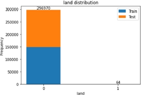
Figure 8.1. Land category distribution
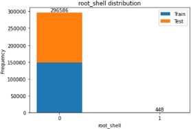

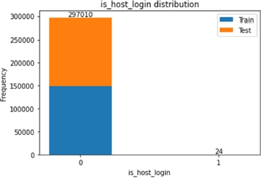

Figure 8.5. Is_guest_login category distribution
The target column (“class”) is also a binary feature, which indicates whether a connection was classified as “normal” or “anomalous”. Figures 8.6 and 8.7 show the number of normal and anomalous samples that were contained in the train and test sets. As we can see, the target variable (class) has a nearly even distribution of values throughout the dataset, meaning that there are a lot of anomalous examples that can be used for training.
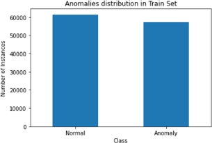
Figure 8.6. Distribution of the target column values in the train set
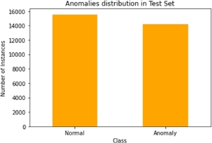
Figure 8.7. Distribution of the target column values in the test set
8.2.4. Categorical features distribution
The NSL-KDD dataset contains a few multi-class categorical features, which are used to label each connection with its protocol, service and other useful characteristics, for example, if the user tried to gain super-user access.
Figures 8.8 – 8.13 describe, for each categorical feature, how many occurrences of each label are present in both the train and the test set. Note that class, protocol type, service and flag features contain textual values, while all other categories are expressed by a number.

Figure 8.8. Protocol type value distribution
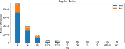
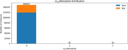

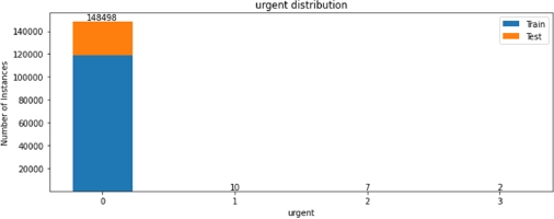
We can see that some of the categories are not evenly distributed, with more than 99% of the sample belonging to just one class, for example, only 84 among more than 148,000 connections have tried to gain root access. This kind of analysis will be useful during the feature selection step, when we will try to identify which categorical feature carries more information about anomalies.
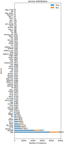
Figure 8.13. Service value distribution
8.2.5. Numerical data distribution
Numerical features have very different meanings in this dataset, and consequently different ranges. Continuous features are used for rates (e.g. error rates), which range from 0.0 to 1.0, and discrete features give information about the number of bytes in the packet, the connection duration, the number of reconnections and many other.
Figure 8.14 represents the normalized dataset: each column’s value has been normalized between 0 and 1 to visualize how the different values of each feature are distributed.
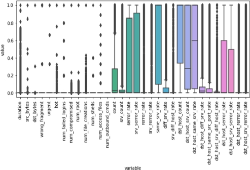
Figure 8.14. Distribution of discrete and continuous features inside the normalized dataset
Note that this normalization considers both the train and the test set, which is not a realistic scenario and is done only in this preliminary phase for data visualization purposes.
8.2.6. Correlation matrix
As a final step of the data analysis, we run a correlation analysis for all the features of the dataset. Figure 8.15 illustrates this correlation matrix.
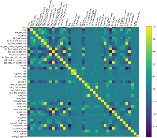
Figure 8.15. Correlation matrix of all the features of the dataset. A lighter color means higher correlation
Focusing on the class column, we can see how each feature is correlated with the target variable, either directly or inversely. This analysis can be extremely useful when performing feature selection to estimate how many important features are there in the dataset.
8.3. Data preparation
In this section, we will describe all the techniques used for cleaning and preparing the data for the learning phase.
8.3.1. Data cleaning
Since the NSL-KDD dataset is already an enhanced version of the older KDD ‘99 CUP dataset, little additional cleaning had to be performed: the set is already cleaned from redundant data and null values (Dhanabal and Shantharajah 2015).
The ratio between normal and anomalous entries is also good for machine learning purposes.
The only cleaning action that should be taken at this step, after loading the arff files and encoding strings in UTF-8, is to remove the num_outbound_commands column, which is filled with only “0”s.
8.3.2. Categorical columns encoding
After cleaning the dataset, the second step is to convert all categorical columns into one-hot encoded columns. This means that, for each distinct value of each categorical column, a new column is generated, containing “1” for the rows belonging to that category and “0” elsewhere.
This kind of encoding is the most popular choice when it comes to preparing data for ANN learning (Potdar et al. 2017). This is done to prevent the algorithm from interpreting categories as numbers, which can lead to problems such as the algorithm considering a category the mean of other two categories, which is clearly not what we want. The affected columns are:
- – service;
- – protocol type;
- – super-user attempted;
- – flag;
- – wrong fragment;
- – urgent.
The dataset resulting from this encoding contains 130 columns, of which one is the target columns.
Note that binary columns are not affected by the encoding. This is to avoid redundant columns, since binary features would have two corresponding encoded columns, in which one can be directly inferred by observing the other. Adding such columns would only increase the dataset noise and size, without adding useful information for the ANN.
8.3.3. Normalization
Having encoded the categorical columns, now the numerical columns must be treated.
Continuous features are already expressed with numbers from 0 to 1, so they all have the same scale. On the other side, discrete columns, which describe features such as the number of bytes exchanged and various counters, contain positive integers of different scales.
On this column we apply a normalization function, for two main reasons:
- – To reduce all features to the same scale: when analyzing a particular instance in a classification problem, we are not interested in the absolute value that is contained in a feature, but instead we want to know what this value means with respect to others. This avoids the possibility of the neural network giving more weight to bigger numbers.
- – To soften the impact of outliers: some of the recorded data in the dataset contain extreme values, for example, very long packets or very long connections. These extreme values represent exceptional cases, but, on the other hand, we want our ANN to be able to recognize primarily the most common cases.
For this reason, we decided to use scikit-learn’s Normalizer2, which rescales the vector for each sample to have unit norm, independently of the distribution of the samples. The normalization process has been accomplished as follows:
- – fit the model onto the train set;
- – transform the train set;
- – transform the test set (with the same normalization model).
Figure 8.16 shows the distribution of the numerical values in the train set after normalization, while Figure 8.17 illustrates the same transformation applied to the test set.
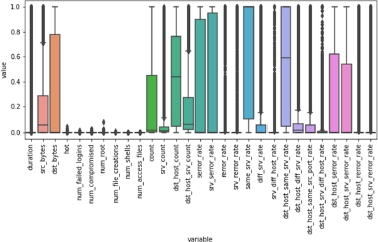
Figure 8.16. Distribution of the values of each numerical feature in the normalized train set
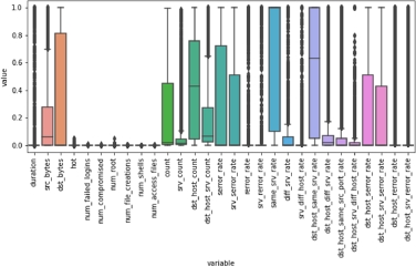
Figure 8.17. Distribution of the values of each numerical feature in the normalized test set
As an example of the behavior of this scaler, Figures 8.18–8.21 show the distribution of the values of two features before and after normalization.

Figure 8.18. Distribution of src_bytes before normalization
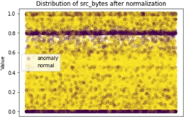
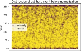
Figure 8.20. Distribution of dst_host_count before normalization
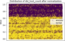
Figure 8.21. Distribution of dst_host_count after normalization
8.4. Feature selection
As a final step of our data preparation pipeline, we want to reduce the number of features over which the ANN should reason, that is perform feature selection. Feature selection in our case has two main purposes: reduce the problem complexity and reduce overfitting.
Since the one-hot encoding increased the number of features considerably, reducing the problem complexity can significantly impact speed and performance, especially during the ANN training phase.
By reducing the information on the train set, we also reduce the possibility of overfitting, since we are omitting specific information of the initial data while trying to concentrate only on the most useful features. However, if not correctly performed, feature selection can introduce some losses in terms of the accuracy of the final output.
Many algorithms are available today for performing feature selection (Huang 2015), each with different tradeoffs. For our IDS, we chose to try two commonly employed methods: univariate selection and tree-based selection.
8.4.1. Tree-based selection
Tree-based selection methods use decision trees to derive the impurity of each feature. This information can then be used to select important features in the dataset. In particular, a random forest of classification trees is built: the idea is to construct a great number of decision trees that see only a random extraction of the features of the initial dataset. Each tree will then construct its nodes, each of which will try to split the dataset into two sets of similar nodes. Calculating the impurity of the resulting sets for each feature, and averaging them out over the trees, we obtain the final importance of the variable.
To perform this kind of selection, we employ ExtraTreesClassifier, which is a classification algorithm provided by Python’s scikit-learn library3. Figure 8.22 shows the ranking of the best features obtained when running the classifier on the train set.

Figure 8.22. Top features ranked by importance found by the ExtraTrees Classifier
8.4.2. Univariate selection
Univariate feature selection is another common method for feature selection. It uses univariate statistical tests, such as chi-squared and F tests, from which we can obtain univariate scores and p-values. This method essentially differs from the tree-based method, since in the latter the forest is constructed randomly.
For our classification problem, the chi-squared statistical test is employed to measure the strength of the relationship of the feature with the target variable. The implementation used is provided by the scikit-learn collection4. Figure 8.23 shows the best 30 features found with univariate selection.
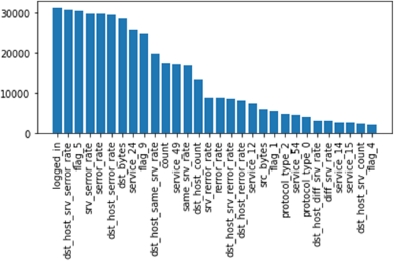
Figure 8.23. Top 30 features ranked by importance found by univariate selection
As we can see, the two methods have selected different sets of features. We will compare the results of these decisions in later sections.
8.5. Model design
8.5.1. Project environment
All results collected in this work have been generated building neural networks in Python 3.6. To build the ANN model, the Keras library has been employed, with TensorFlow as a backend. Therefore, many hyperparameters and specific implementations are provided by these frameworks.
8.5.2. Building the neural network
The approach for constructing the neural network for this work has been to try different combinations of layers and see how each model performs in terms of accuracy and loss, comparing these two metrics for the train and test set.
All neural networks have been implemented in Keras5 using the sequential (i.e. feed-forward) model and dense (i.e. fully interconnected) layers. Following the work of (Kim and Gofman 2018), the tested models consist of both shallow networks and deep networks with up to four hidden layers.
8.5.3. Learning hyperparameters
When designing a neural network there are many hyperparameters that have to be set apart from the number of layers and neurons in each layer. In particular, the following parameters were chosen after some initial tests:
- – Learning rate: In order to keep a good convergence without losing accuracy, this parameter has been set to 0.001. Other values tried were 0.01 and 0.0001.
- – Optimization algorithm: Adam6, one of the standard optimizers provided by Keras.
- – Loss function: Binary-crossentropy. This was chosen since we are building a binary classifier.
8.5.4. Epochs
Each model was trained with a fixed number of epochs, which were empirically chosen to be 150.
In future developments, fixed epochs could be substituted by early stopping to speed up the learning phase: in this way, the training would stop whenever the accuracy cannot be significantly improved, and this can happen much before the 150th epoch.
8.5.5. Batch size
Choosing the batch size implies a tradeoff between the speed of the learning phase and the accuracy of the model. A batch size of 1, sometimes called online learning, means that, for each epoch of the learning phase, the input data will be learned one entry at a time.
Having a batch size which is much smaller than the entire dataset but still greater than one, such as 16 or 32 (sometimes called mini-batch), means that more than one entry will be analyzed together in a single step of a learning epoch.
It has been shown in Keskar et al. (2016) that this solution might be preferable in general with respect to larger batches, so our choice has been to set the batch size to 16.
8.5.6. Dropout layers
Dropout regularization is a common and well-established method to prevent models from overfitting (Srivastava et al. 2014). This method consists of adding dropout layers to the neural network. These layers are interposed between the other layers of the network, and their effect is to inhibit the output of the previous layer with a certain probability. This is equivalent to randomly discarding some of the effects of the input during the training phase, which makes the model more robust and immune to overfitting.
The probabilities chosen are:
- – Input layer: 0.5. A high dropout probability in the input layers means that not all features will be used for all the data, which is the primary idea when trying to avoid overfitting.
- – Hidden layers: 0.2.
Other probabilities have been tried, such as 0.8 for the input layer and 0.5 for the hidden layers, but the results of the model were degraded. See section 8.6.4 for a more detailed analysis of the results.
8.5.7. Activation functions
For the hidden layers, different activation functions have been tried in the shallow versions of the network to verify their effect on the final classifier. The standard activation functions were tried: relu, tanh and sigmoid. Section 8.6.2 contains the results of the different experiments done with different activation functions.
The input and output layers were instead held at a fixed activation function: relu for the input and sigmoid for the output.
8.6. Results comparison
Different models have been tested to compare different solutions and find the best fit for this task. This section provides a comparison between the performances of each neural network model built.
Each model comes with a description of its shape (i.e. number of layers and units per layer), the training history (loss and accuracy in each epoch) and the results on the test set (confusion matrix).
For the learning and validation steps, the NSL-KDD dataset was divided into a train set containing 125,973 instances (≈85%) and test set containing 22,544 instances (≈15%). We also used 15% of the train set as dev set, in order to keep track and plot the accuracy and loss of each model during the training phase.
8.6.1. Evaluation metrics
The most common evaluation metrics for IDS, as reported by (Thomas and Pavithran 2018), are Attack Detection Rate (DR) and False Alarm Rate (FAR).
We can calculate these metrics from the confusion matrix, which is represented by the following terms:
- – True Positive (TP): the instance is correctly predicted as an attack.
- – True Negative (TN): correctly predicted as a non-attack or normal instance.
- – False Positive (FP): a normal instance is wrongly predicted as attacks.
- – False Negative (FN): an actual attack is wrongly predicted as a non-attack or normal instance.
False positives happen when a normal network activity is classified as an attack, and can waste the valuable time of security administrators.
False negatives, on the other hand, have the worst impact on organizations since an attack is not detected at all.
8.6.2. Preliminary models
As a preliminary step, three shallow networks consisting of just two layers (excluding the output node) were built with different activation functions. These neural networks have been trained with no dropout layers, no feature selection (all 128 features were used) and a smaller number of epochs (50). The idea is to look at the various results as well as learning curves and pick an activation function for later models. The results are reported in the following sections.
8.6.2.1. Shallow network with “relu” activation
As a first attempt, we built a shallow network with two hidden layers and “relu” as activation function for the hidden layers’ neurons. Figure 8.24 shows the learning curves of the model, plotted during the learning phase, while Table 8.3 contains information about the shape of the network and its results on the test set.
The results are already interesting, but we can see from the learning curves that the model starts overfitting fairly early.
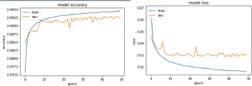
Figure 8.24. Learning curves (accuracy and loss) of the first model (all features, no dropout, relu activation function for hidden layers)
Table 8.3. Shape and results of the first model
Input Features | Input Dropout | Layer 1 | Layer 2 | Hidden Layers Dropout | DR | FAR |
128 | None | 30, relu | 10, relu | None | 99.20% | 0.93% |
8.6.2.2. Shallow network with “tanh” and “sigmoid” activation
For comparison purposes, we also tried the same network with “tanh” and “sigmoid” as activation function for the second layer. Figures 8.25 and 8.26 show the learning curves of these models, while Table 8.4 contains the results.
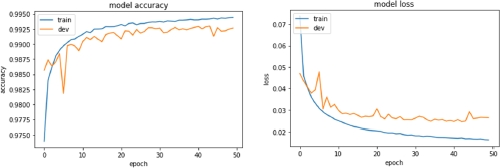
Figure 8.25. Learning curves (accuracy and loss) of the second model (all features, no dropout, tanh activation function for hidden layers)
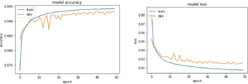
Figure 8.26. Learning curves (accuracy and loss) of the third model (all features, no dropout, sigmoid activation function for hidden layers)
Table 8.4. Shape and results of the second and third models
Input Features | Input Dropout | Layer 1 | Layer 2 | Hidden Layers Dropout | DR | FAR |
128 | None | 30, relu | 10, tanh | None | 99.44% | 1.05% |
128 | None | 30, relu | 10, sigmoid | None | 99.41% | 1.00% |
8.6.2.3. Conclusions
After this preliminary phase, we can conclude that the generated models have a very similar accuracy. We choose to base the other models on the best we found in this phase, that is, use tanh as activation function for the hidden layers.
8.6.3. Adding dropout
Having decided the activation function, it is now the moment to decide the dropout probability associated with the dropout layers. Fixing the dropout rate too low would give us little benefit in terms of avoiding overfitting. On the other hand, having a dropout rate that is too high might introduce performance degradation in to the model.
Here we tried out three possible pairs of rates:
- – aggressive dropout: input dropout 0.8, 0.5 for other layers;
- – intermediate dropout: input dropout 0.5, 0.2 for other layers;
- – low dropout: input dropout 0.3, 0.1 for other layers.
The results of these experiments are reported in Table 8.5.
Table 8.5. Shape and results of the dropout models
Input Features | Input Dropout | Layer 1 | Layer 2 | Hidden Layers Dropout | DR | FAR |
128 | 0.8 | 30, relu | 10, tanh | 0.5 | 99.12% | 4.54% |
128 | 0.5 | 30, relu | 10, tanh | 0.3 | 99.31% | 1.09% |
128 | 0.3 | 30, relu | 10, tanh | 0.1 | 99.17% | 0.88% |
Looking at the learning curves we can see that the model is effectively overfitting less on the training set. Figure 8.27 shows the learning curve for the low dropout model.
This is an important result, since we want our model to be able to recognize previously unknown or unidentified violations in our systems, hence we cannot expect the training set to contain all the possible attacks.
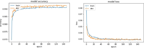
Figure 8.27. Learning curves (accuracy and loss) of the low dropout model
8.6.4. Adding more layers
Another typical choice that has to be made when designing a neural network is the number of layers and neurons in a layer.
Here we compare deeper models, that is, models with more layers, to the previously constructed ones, and we compare the results.
Table 8.6 shows the resulting accuracy and false alarm rate for the constructed models.
8.6.5. Adding feature selection
As a final step for our model design phase, we reduce our dataset using the techniques described in section 8.3.3 (ExtraTrees Classifier with a random forest and univariate selection using chi-squared statistical tests).
The resulting models are much lighter versions of the previous ones, which can be trained in less time.
Table 8.7 contains the results of the two selection algorithms in two different models: a shallow one and a deep one.
Table 8.7. Comparison between models trained on ExtraTrees Classifier selected features and on univariate selection selected features
Input Features | Selection | Input Dropout | Layer 1 | Layer 2 | Layer 3 | Hidden Dropout | DR | FAR |
31 | ExtraTrees | 0.3 | 30, relu | 10, tanh | None | 0.1 | 99% | 1.24% |
31 | ExtraTrees | 0.3 | 30, relu | 30, tanh | 10, tanh | 0.1 | 99.07% | 1.04% |
30 | Univariate | 0.3 | 30, relu | 10, tanh | None | 0.1 | 98.79% | 1.08% |
30 | Univariate | 0.3 | 30, relu | 30, tanh | 10, tanh | 0.1 | 98.61% | 1.02% |
8.7. Deployment in a network
This section describes which steps should be made to deploy one or more of the produced models in a real network environment.
8.7.1. Sensors
To deploy an IDS in a real network, the first components we need are sensors that can record traffic and produce the tuples that will be then fed into the model. Sensor placement is a key factor for an IDS to be able to protect the network from invasion. For this task, the network architecture should be studied in detail, to observe all possible points of entrance.
Depending on how large and complex our network is, we can choose to deploy the whole system in a single device, as suggested by Kim and Gofman (2018), or implement multiple sensors, as done in Chen et al. (2010). In both cases, the most sensitive points to place the sensors are typically before and after each router or DMZ of the network. Figure 8.28 describes this situation.
In general, IDS sensors have two network interfaces – one for monitoring traffic and one for management. The traffic monitoring interface is unbound from any protocol, which means that the interface has no IP address and other entities cannot communicate with it. This guarantees that no attack surface is exposed on the network by the sensor itself.
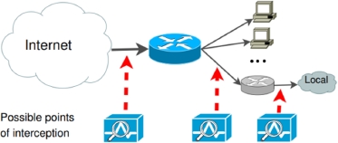
Figure 8.28. Possible points of interception for an NIDS
(source: Kim et al. (2012))
8.7.2. Model choice
After deploying the sensors, we must choose which model to deploy. The model choice can depend on evaluation metrics like detection rate or false alarm rate but should also consider the model complexity. A higher model complexity can imply a higher cost for data acquisition and greater delays for the system’s response.
This kind of analysis shall be done also taking into consideration the response time of each model, which is outside the scope of this work. For reducing the complexity, we can employ one of the feature selection methods previously described in this chapter.
8.7.3. Model deployment
Once the IDS is deployed in the network, we want it to work with streams of incoming data in a fully automated way. This implies several steps, which are described in Figure 8.29.
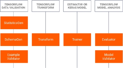
Figure 8.29. Possible steps of the IDS once deployed in a real system
There are many possible solutions to achieving this automation which range from fully personalized solutions to fully COTS products. One simple possibility, since the models of this work have been trained using TensorFlow, is to use TensorFlow Extend7, a collection of tools used for deploying ANN models in the wild. Figure 8.30 describes the components of the TFX framework, which range from data cleaning to Keras model validation.
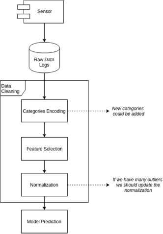
Figure 8.30. Components of the TFX framework as described in the official guide
On line deployment can be achieved by using TensorFlow Serving8, which is a framework built to enable fast TensorFlow models’ deployment over REST APIs. TF Serving also has the ability to deploy a model to a Docker image and use Kubernetes to manage a cluster of these images running together. This offers a good solution in terms of scalability of the IDS, which can easily keep up with a possible growth of the network that it is protecting.
8.7.4. Model adaptation
Once it is online, the model should then be trained and updated with real data coming from the network. This is a time-consuming task, which requires the network to be in a temporary “safe” state in which the model can learn what the normal behavior of the system is.
After the training time, the IDS is ready to be used in the network environment. To extend the training time, a human supervisor can be assigned to check the entries that are signaled as anomalous and re-labeling them if necessary. The same model can also be periodically retrained with a larger dataset or with only the latest entries.
8.8. Future work
This work represents only a preliminary analysis of how an NIDS can be modeled and deployed using ANN and TensorFlow. Many improvements can be made to the models to achieve better performances, such as implementing early stopping instead of a fixed number of epochs and adapting the Keras model to work with TPUs (Tensor Processing Units), which can significantly improve the training time needed.
An in-depth analysis of a target network should also be performed to deploy the IDS in a real network. Problems such as the efficiency, delay and the sample collection in the new network environment are specific to each network and must be considered if we want to carry out the IDS deployment.
8.9. References
Chen, H., Clark, J.A., Shaikh, S.A., Chivers, H., Nobles, P. (2010). Optimising IDS sensor placement. ARES ‘10 International Conference on Availability, Reliability and Security, IEEE, 315–320.
Dhanabal, L. and Shantharajah, S.P. (2015). A study on NSL-KDD dataset for intrusion detection system based on classification algorithms. International Journal of Advanced Research in Computer and Communication Engineering, 4(6), 446–452.
Huang, S.H. (2015). Supervised feature selection: A tutorial. Artificial Intelligence Research, 4(2), 22–37.
Keskar, N.S., Mudigere, D., Nocedal, J., Smelyanskiy, M., Tang, P.T.P. (2016). On large-batch training for deep learning: Generalization gap and sharp minima. CoRR [Online]. Available at: https://arxiv.org/abs/1609.04836.
Kim, S., Nwanze, N., Edmonds, W., Johnson, B., Field, P. (2012). On network intrusion detection for deployment in the wild. IEEE Network Operations and Management Symposium, 253–260.
Kim, D.E. and Gofman, M.I. (2018). Comparison of shallow and deep neural networks for network intrusion detection. 2018 IEEE 8th Annual Computing and Communication Workshop and Conference (CCWC), 204–208.
Lazarevic, A., Ertoz, L., Kumar, V., Ozgur, A., Srivastava, J. (2003). A comparative study of anomaly detection schemes in network intrusion detection. In Proceedings of the 2003 SIAM International Conference on Data Mining, Society for Industrial and Applied Mathematics, 25–36.
Mukherjee, B., Heberlein, L.T., Levitt, K.N. (1994). Network intrusion detection. IEEE Network, 8(3), 26–41.
Potdar, K., Pardawala, T., Pai, C. (2017). A comparative study of categorical variable encoding techniques for neural network classifiers. International Journal of Computer Applications, 175(4), 7–9.
Reddy, E.K. (2013). Neural networks for intrusion detection and its applications. Lecture Notes in Engineering and Computer Science: Proceedings of the World Congress on Engineering 2013, International Association of Engineers, 2(205), 1210–1214.
Srivastava, N., Hinton, G., Krizhevsky, A., Sutskever, I., Salakhutdinov, R. (2014). Dropout: A simple way to prevent neural networks from overfitting. Journal of Machine Learning Research, 15(56), 1929–1958.
Subba, B., Biswas, S., Karmakar, S. (2016). A neural network based system for intrusion detection and attack classification. Twenty Second National Conference on Communication (NCC), IEEE, 1–6.
Thomas, R. and Pavithran, D. (2018). A survey of intrusion detection models based on NSL-KDD data set. 2018 Fifth HCT Information Technology Trends (ITT), IEEE, 286–291.
- For a color version of all the figures in this chapter, see: www.iste.co.uk/chelouah/optimization.zip.
- 1 https://www.unb.ca/cic/datasets/nsl.html.
- 2 https://scikit-learn.org/stable/modules/generated/sklearn.preprocessing.Normalizer.html.
- 3 https://scikit-learn.org/stable/modules/generated/sklearn.ensemble.ExtraTreesClassifier.html.
- 4 https://scikit-learn.org/stable/modules/generated/sklearn.featureselection.SelectKBest.html#sklearn.feature_selection.SelectKBest.
- 5 https://keras.io.
- 6 https://www.tensorflow.org/apidocs/python/tf/keras/optimizers/Adam.
- 7 https://www.tensorflow.org/tfx.
- 8 https://www.tensorflow.org/tfx/guide/serving.