
3
Solving Feature Selection Problems Built on Population-based Metaheuristic Algorithms
Mohamed SASSI
PJGN IT Director, Gendarmerie Nationale, France
Machine learning classifiers require a large amount of data for the training, validation and testing phases. These data are generally high dimensional. However, the higher the dimension, the more the performance of the classifier deteriorates due to the huge quantity of irrelevant and correlated data and noise, without mentioning the curse of the dimension. The effect on machine learning algorithms is detrimental: overfitting, high complexity, high computational cost and poor accuracy. The corollary is that in order to obtain a better performance, an efficient feature selection process must be implemented. However, feature selection is also an optimization problem. Therefore, nature-inspired and population-based metaheuristics, such as the grey wolf optimization (GWO) algorithm, are one of the best solutions to this problem. This chapter allows us to demonstrate step by step, in a pedagogical way, the use of the GWO for the feature selection process applied on a KNN (k-nearest neighbor) classifier with very competitive results compared to the GA and PSO metaheuristics.
3.1. Introduction
The 21st century has seen an exponential increase in the amount of data, irrespective of the professional sectors: forensics, medicine, meteorology, finance, astrophysics, agronomy, etc. This huge mass of data results in errors within even the most sophisticated machine learning algorithms.
However this observation does not spell disaster, thanks to feature selection algorithms. These algorithms extract a subset of data containing the most meaningful information. Nevertheless, feature selection is an NP-difficult multi-objective optimization problem (Fong et al. 2014; Siarry 2014; Hodashinsky and Sarin 2019). Extensive research in this area has shown the superiority of metaheuristic algorithms in solving these problems compared to other optimization algorithms, such as deterministic methods (Sharma and Kaur 2021). Population-based swarm intelligence metaheuristics have been shown to be effective in this area.
Unfortunately we have found very few book chapters dedicated to the study of metaheuristics, and which actually describe the operation of metaheuristics for feature selection. Metaheuristics are powerful tools for these data processing steps.
In this chapter, we do not create a new metaheuristic. Our contribution is to explain, in an educational way, all the steps required to apply a modern metaheuristic in a continuous research space to feature selection. To do this, we rely on the work of Mirjalili and of Emary (Mirjalili et al. 2014; Emary et al. 2016).
This chapter is organized into eight sections as follows. Section 3.2 presents inspiration from the nature of the GWO algorithm. Section 3.3 develops a mathematical model of the GWO for optimization in a continuous search space. Section 3.4 allows us to assimilate the theoretical fundamentals of feature selection. Section 3.5 discusses the mathematical modeling of optimization in a binary discrete search space. Section 3.6 provides the binarization modules allowing continuous metaheuristics to be able to solve feature selection problems in a binary search space. Section 3.7 is the heart of this chapter because it uses the binarization modules of section 3.6 to create the binary metaheuristics bGWO. Section 3.8 will demonstrate, experimentally, the performance of bGWO in solving feature selection problems on 18 datasets from UCI reference datasets.
3.2. Algorithm inspiration
The grey wolf belongs to the Canis lupus (Canidae) family. Over the centuries, since their appearance about two million years ago, wolves have developed and perfected their hunting technique. Their existence on several continents is evidence that this hunting technique is optimal for finding the best prey; it thus inspired the GWO algorithm, which is based on the hierarchical organization of the pack as well as the four phases of the hunt.
3.2.1. Wolf pack hierarchy
The keystone of the grey wolf pack is its hierarchy, which is structured into four groups: Alpha, Beta, Delta and Omega (Figure 3.1).
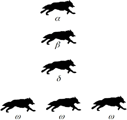
Figure 3.1. Wolf pack hierarchy
3.2.1.1. Alpha wolf
An Alpha male wolf pairs with an Alpha female wolf to form an Alpha pair. These Alpha wolves lead the pack, taking charge of hunting, meals, reproduction and defense. They therefore ensure the success of the pack.
3.2.1.2. Beta wolf
The Beta wolf assists the Alpha wolves. They will become the Alpha if the latter is no longer able to fulfill their role. On a daily basis, they assist the Alpha wolves in commanding and maintaining order in the pack.
3.2.1.3. Delta wolf
The Delta wolf is ranked lower than the Beta wolf. Much like the Beta, they help its Alpha and Beta superiors in day-to-day tasks and in maintaining discipline in the ranks.
3.2.1.4. Omega wolf
Omega wolves are at the bottom of the pack hierarchy. They obey and follow the Alpha, Beta and Delta and bear the brunt of any suffering within the pack. Aside from the Alpha, Beta and Delta, the rest of the wolves in the pack are all Omega.
The Alpha, Beta, Delta and Omega hierarchy is thus an expression of the methodical rigor of grey wolf pack life. Applying this methodical rigor is most crucial when the pack executes its hunting technique.
3.2.2. The four phases of pack hunting
The grey wolf pack hunts their prey by progressing through four phases, as illustrated in Figure 3.2:
- 1) search;
- 2) pursue;
- 3) surround and harass the prey until trapped or exhausted;
- 4) attack the prey.
The hierarchy of the pack and the four phases of its hunting technique constitute the two pillars of the GWO metaheuristic. These are modeled mathematically in the next section.
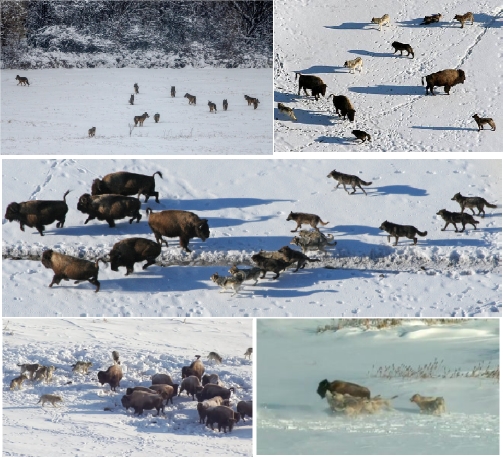
Figure 3.2. Search, pursue, surround-harass and attack the prey
(source: https://phys.org (ecologists larger group)). For a color version of this figure, see www.iste.co.uk/chelouah/optimization.zip
3.3. Mathematical modeling
3.3.1. Pack hierarchy
Wolf agents Alpha, Beta and Delta (Figure 3.3) are the most important wolves in the pack and assume prime position when surrounding prey during hunting (Figure 3.4). They will therefore be respectively the first, second and third best solutions to the optimization problem. The Omega wolves alter their position based on the positions of the Alpha, Beta and Delta.
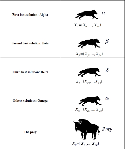
Figure 3.3. Pack hierarchy modeling

Figure 3.4. Alpha, Beta, Delta and Omega Wolf positions around prey
(source: https://phys.org (ecologists larger group)). For a color version of this figure, see www.iste.co.uk/chelouah/optimization.zip
3.3.2. Four phases of hunt modeling
3.3.2.1. Search and pursue
This phase involves searching for and then pursuit of the most promising areas in which to hunt for prey. It is the GWO exploration phase. As a result of these phases, the three best solutions will create the hierarchy of the pack: Alpha, Beta and Delta. They will lead the encirclement and harassment phases.
3.3.2.2. Encirclement and harassment
The encirclement and harassment of prey by wolf agents are modeled by equations [3.1]–[3.5].
- – t indicates the current iteration;
- –
 (t) is the Omega wolf position at iteration t ;
 - – (t+1) is the Omega wolf position at the next iteration t + 1
- –
 is the prey position;
 - –
 ,
,  and
and  are vectors defined by equations [3.3], [3.5] and [3.1];
 - – a is a coefficient that decreases linearly from 2 to 0 in terms of until maximum iteration itMax.
Vectors ![]() ,
, ![]() and
and ![]() are calculated as follows:
are calculated as follows:
Based on equations [3.1] and [3.2] in a search area of size N, wolf agents evolve in a hypercube around the prey (the best solution). Figures 3.5 and 3.6 graphically illustrate the hypercube created by a wolf around the prey before the attack with equations [3.1] and [3.2] for N = 2 and N = 3, respectively. In the attack equations [3.6]–[3.12], the position of the prey is represented by the three best solutions at the iteration t: Alpha, Beta and Delta. Therefore, three hypercubes will be created for each of them.
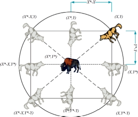
Figure 3.5. Position of the wolf agent and its prey in a square with N = 2 (Mirjalili et al. 2014). For a color version of this figure, see www.iste.co.uk/chelouah/optimization.zip
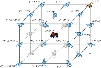
Figure 3.6. Position of the wolf agent and its prey in a cube with N = 3 (Mirjalili et al. 2014) . For a color version of this figure, see www.iste.co.uk/chelouah/optimization.zip
3.3.2.3. Attack
According to the social order established by the hierarchy of the pack, the Alpha, Beta and Delta wolf agents guide the attack. The postulate of the pack is based on the principle that the hierarchy has a better perception of the position of prey. Therefore, the Omega will update their position ![]() from the encirclement areas around the prey, created by the positions of the Alpha, Beta and Delta:
from the encirclement areas around the prey, created by the positions of the Alpha, Beta and Delta: ![]() .
.
To do this, equations [3.1] and [3.2] are used with positions ![]() ,
, ![]() and
and ![]() to obtain
to obtain ![]() ,
, ![]() ,
, ![]() in the encirclement areas of the Alpha, Beta and Delta.
in the encirclement areas of the Alpha, Beta and Delta. ![]() ,
, ![]() ,
, ![]() are provided by equations [3.6], [3.9] and [3.11]. The wolf agents will update their position
are provided by equations [3.6], [3.9] and [3.11]. The wolf agents will update their position ![]() on the mean of
on the mean of ![]() ,
, ![]() and
and ![]() with equation [3.12]. This update allows the pack to approach the best solutions.
with equation [3.12]. This update allows the pack to approach the best solutions.
The vectors ![]() and
and ![]() are strategic random vectors for the GWO algorithm. Indeed, their stochastic nature supports the exploration phase.
are strategic random vectors for the GWO algorithm. Indeed, their stochastic nature supports the exploration phase. ![]() is the vector that leads the exploration and exploitation phases.
is the vector that leads the exploration and exploitation phases. ![]() stochastically models the obstacles between the wolf and the prey.
stochastically models the obstacles between the wolf and the prey. ![]() also plays a fundamental role in the exploration and exploitation phases. The closer |
also plays a fundamental role in the exploration and exploitation phases. The closer |![]() | is to 2, the more complex it will be to attack the prey and therefore the more the wolf will have to explore other areas around the prey in order to access it. On the other hand, the closer |
| is to 2, the more complex it will be to attack the prey and therefore the more the wolf will have to explore other areas around the prey in order to access it. On the other hand, the closer |![]() | is to 0, the closer the wolf is getting to the area around the prey that favors exploitation.
| is to 0, the closer the wolf is getting to the area around the prey that favors exploitation.
For example, if N = 2, the equations [3.6] and [3.7] are calculated as follows:
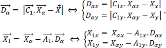
By doing the same for ![]() the next agent position is:
the next agent position is: 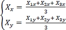
3.3.3. Research phase – exploration
The search for prey requires wolves to occupy the search area by spreading out. When |A| ≥ 1, the wolf agents are in the exploration phase which involves a random search for promising areas. The wolf agents change positions by dispersing and are therefore better placed to find new promising zones around prey.
|C| is stochastic and randomly evolves from 0 to 2. If |C| ≥ 1, it removes the wolf agents from the prey and promotes exploration.
3.3.4. Attack phase – exploitation
Attacking prey is the exploitation phase of the hunt when 1 > |A| ≥ 0. Indeed, in this interval, the wolf agents will progress toward the prey by getting closer to one another.
If |C| < 1, the wolf agents are brought closer to the prey after overcoming obstacles and this promotes exploitation.
Figure 3.7 graphically illustrates the evolution of A between exploration and exploitation phases and Figure 3.8 shows the position of the wolf in relation to the prey in the exploration and exploitation phase.
It can be noted that the first half of the iterations, when ![]() , promotes the exploration with 2 ≥ a ≥ 1 , and the second half, when
, promotes the exploration with 2 ≥ a ≥ 1 , and the second half, when ![]() , promotes the exploitation with 1 > a ≥ 0.
, promotes the exploitation with 1 > a ≥ 0.
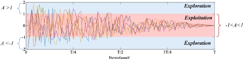
Figure 3.7. Steering of exploration and exploitation phases with vector A during iterations (Faris et al. 2017) . For a color version of this figure, see www.iste.co.uk/chelouah/optimization.zip
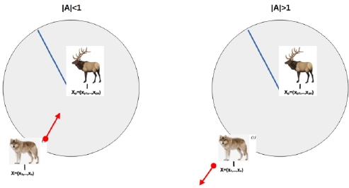
Figure 3.8. Search exploration phase |A|≥1 and attack exploitation phase 1>|A|≥0. For a color version of this figure, see www.iste.co.uk/chelouah/optimization.zip
3.3.5. Grey wolf optimization algorithm pseudocode
We now have all the elements allowing us to understand the mathematical modeling of the GWO algorithm. The understanding and mastery of the key points of this algorithm is an imperative for the remainder of this chapter. In the following section, we are going to approach the main topic of this chapter: feature selection. We must first know the theoretical fundamentals of feature selection and optimization in a binary discrete search space.
3.4. Theoretical fundamentals of feature selection
Machine learning classification algorithms are a component of artificial intelligence that require maximum reactivity to the data mass they need to process. They must therefore be reactive, accurate, adaptive and as light as possible. To do this, we must provide the algorithm with only the data necessary for its decision-making so as not to swamp it with redundant or irrelevant data. This is the purpose of feature selection. This section will provide the theoretical fundamentals of feature selection as well as the main advantages of feature selection for the machine learning classifiers.
3.4.1. Feature selection definition
Feature selection is the problem of how to choose the fewest features in the original dataset that are often high-dimensional (Almomani et al. 2019). It is therefore an extraction process that eliminates irrelevant and redundant features for a better understanding of datasets (Sharma and Kaur 2021). In practice, feature selection consists of exploiting ad hoc algorithms for processing a dataset with N features as the input and providing at the output a subset of p feature data with p < N. Figure 3.9 illustrates this process. But what are the methods to achieve it?
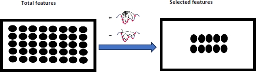
Figure 3.9. Feature selection process. For a color version of this figure, see www.iste.co.uk/chelouah/optimization.zip
3.4.2. Feature selection methods
There are two main feature selection algorithm families: chaotic and binary (Sharma and Kaur 2021). The binary feature selection is the most used in the literature thanks to its good performance and a better theoretical and practical control. It is therefore the binary selection that we will implement in this chapter.
The binary feature selection family has two predominant types of feature selection methods: the filter method and the wrapper method (Chandrashekar and Sahin 2014; Almomani et al. 2019; Sakr et al. 2019; Sharma and Kaur 2021).
3.4.3. Filter method
The filter method is independent of the optimization problem and classifier; its key advantage. It uses statistical algorithms that make it possible to calculate a weight for each feature by analyzing any attributes specific to the data. The weights will be compared to a threshold that will provide a feature classification. This ranking will make it possible to delete the feature superior to the threshold. However, this method provides much less precision than selection of the wrapper method. The most used filter methods in the literature are (Sakr et al. 2019):
- – information gain;
- – principal component analysis;
- – characteristics correlation selection.
3.4.4. Wrapper method
The wrapper method uses the machine learning classifier to guide the metaheuristic to lead the feature selection process. This method is therefore adherent to the classifier. In addition, the wrapper method requires more calculation and processing time than the filtering method. However, its main advantage is that it provides better precision and thus better results in solving the feature selection problem. The literature confirms that wrapper methods outperform the filtering methods (Siarry 2014; Sakr et al. 2019; Sharma and Kaur 2021).
In addition, the use of population-based multiple solution metaheuristics provides better results than single solution metaheuristics (Sakr et al. 2019; Sharma and Kaur 2021). The GWO algorithm is therefore suitable for solving the feature selection problem.
Therefore, in this chapter, GWO will be integrated with the wrapper binary feature selection method (Emary et al. 2016). The binary feature selection can be done either by forward selection or by backward elimination.
3.4.5. Binary feature selection movement
The wrapper method allows two feature selection “moves”: forward selection and backward elimination. The selection of forward or backward will depend mainly on the binary vector initialization method chosen.
3.4.5.1. Forward selection
Forward selection consists of starting with a minimum of features and then inserting the features one after another during the selection process until an acceptable error rate is obtained.
3.4.5.2. Backward elimination
Unlike forward selection, the backward elimination process starts with the maximum of features at the start and eliminates them one after another during the selection process, until an acceptable error rate is obtained.
The experimental results explained in section 3.8 demonstrate the qualities of these two selection movements.
3.4.6. Benefits of feature selection for machine learning classification algorithms
The benefits of feature selection on machine learning classification algorithms are multiple. We list the most important here:
- – removal of redundant and irrelevant data;
- – noise reduction;
- – extraction from the curse of the dimension;
- – decrease in classifier complexity;
- – improvement in the quality of supervised learning;
- – increased classification accuracy;
- – decreased classifier response time;
- – material resources saving when running the classifier: memory, CPU, GPU processors and energy.
In view of the benefits listed above, feature selection is a vital step in data processing before the learning phase of a classifier. Being a powerful algorithm for solving NP-hard multi-objective optimization problems, metaheuristics GWO has become one of the keystones in the process of creating a successful classifier. Indeed, feature selection is an NP-hard multi-objective optimization problem in a binary search space. So a modern and powerful metaheuristic like GWO is able to solve this problem. But before developing the binary GWO metaheuristics, we must first know the mathematical modeling of the problem of optimizing feature selection in a binary search space.
3.5. Mathematical modeling of the feature selection optimization problem
In this section, we detail the mathematical environment of the multi-objective feature selection optimization problem: binary discrete search space and objective functions to be minimized. Binary GWO metaheuristics will provide an acceptable solution to this problem within a reasonable time.
3.5.1. Optimization problem definition
Patrick Siarry (Collette and Siarry 2002) defines optimization as “the search for the minimum or the maximum of a given function”. It is therefore a matter of searching in the search space for a data vector which minimizes or maximizes the objective function. The search space of interest to us is the discrete binary search space.
3.5.2. Binary discrete search space
The binary discrete search space is a search space whose vector components can only take the discrete values 0 or 1.
The mathematical representation of a binary vector in the binary search space ![]() N with N features is
N with N features is ![]() .
.
The binary search space ![]() N is represented by a hypercube with 2N vertices. The 2N binary vectors of the search space
N is represented by a hypercube with 2N vertices. The 2N binary vectors of the search space ![]() N are positioned on the vertices. For example, for N=3,
N are positioned on the vertices. For example, for N=3, ![]() 3 is a cube with eight binary vectors positioned on the eight vertices as illustrated in Figure 3.10.
3 is a cube with eight binary vectors positioned on the eight vertices as illustrated in Figure 3.10.
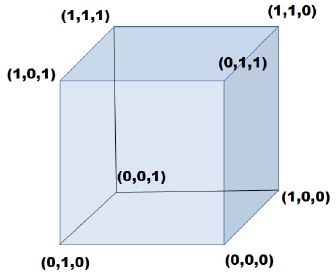
Figure 3.10. Binary search space with N=3
Therefore, there are 2N – 1 solutions for a problem of feature selection with N features. The null vector is ignored because it means to select no features.
Thus, the space research ![]() N exponentially increases with the size of N features. But why would metaheuristics be more appropriate than other algorithms to solve the problem of feature selection? The reason is simple: it is not possible, unless you devote several hours or even several days, to use a deterministic method to solve the problem of feature selection (Zita et al. 2010; Sharma and Kaur 2021). What we need is an acceptable solution within a reasonable wait time. However, the literature abounds with articles demonstrating the effectiveness of population-based metaheuristics, such as GWO.
N exponentially increases with the size of N features. But why would metaheuristics be more appropriate than other algorithms to solve the problem of feature selection? The reason is simple: it is not possible, unless you devote several hours or even several days, to use a deterministic method to solve the problem of feature selection (Zita et al. 2010; Sharma and Kaur 2021). What we need is an acceptable solution within a reasonable wait time. However, the literature abounds with articles demonstrating the effectiveness of population-based metaheuristics, such as GWO.
Before moving on to the next section, we need to understand how to translate a binary vector into a feature selection problem. To do this, let us take the example of a dataset with N = 6. The space research ![]() 6 consists of binary vectors
6 consists of binary vectors ![]() . There are therefore 63 possible solutions. Translating each vector into a feature selection solution in this search space is extremely simple: 0 means that the feature is not selected and 1 means the opposite. Take one of the vertices of the hypercube:
. There are therefore 63 possible solutions. Translating each vector into a feature selection solution in this search space is extremely simple: 0 means that the feature is not selected and 1 means the opposite. Take one of the vertices of the hypercube: ![]() p = (0,1,0,0,1,0) . This vector selects the two features D2 and D5 as illustrated in Figure 3.11.
p = (0,1,0,0,1,0) . This vector selects the two features D2 and D5 as illustrated in Figure 3.11.
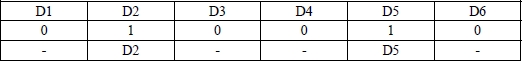
Figure 3.11. Selection vector of features D2 and D5
These binary vectors will be produced by the GWO metaheuristic as input to the objective functions of the feature selection problem.
3.5.3. Objective functions for the feature selection
We have previously stated that a feature selection problem is a multi-objective problem, to be precise a bi-objective problem. Indeed, we must maximize the accuracy of the classifier and minimize the number of selected features. But before setting the two mathematical functions to be optimized, it is necessary to define the vocabulary making it possible to measure the quality of a classifier.
3.5.3.1. Accuracy
Accuracy measures the rate of good classifications. So the higher this rate is, the more the classifier will be able to give us a good answer.
3.5.3.2. Error rate
The error rate is the complement of accuracy. It measures the rate of bad classifications.
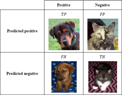
The accuracy and error rate are calculated from the number of true positive TP, true negative TN, false positive FP and false negative FN. Their mathematical definition is respectively provided by the equations [3.13] and [3.17].
To define TP, TN, FP let us take the concrete example of a CNN (convolutional neural network) classifier to detect dogs in pictures.
3.5.3.3. True positive (TP)
This is the number of pictures correctly classified containing a dog.
3.5.3.4. True negative (TN)
This is the number of pictures correctly classified without a dog.
3.5.3.5. False positive (FP)
This is the number of pictures without a dog but classified as containing a dog.
3.5.3.6. False negative (FN)
This is the number of images containing a dog but classified as not containing a dog.
The confusion matrix below illustrates the result of the CNN classification (source image: https://www.kaggle.com/).
Let us now set the two mathematical functions to be optimized.
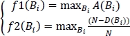
The function A(Bi) is the classifier accuracy depending on the binary vector ![]() and the function D(Bi) is the number of selected features by the binary Bi and N is the feature size. The feature selection problem is defined by equations [3.13]. [3.14] and [3.15]:
and the function D(Bi) is the number of selected features by the binary Bi and N is the feature size. The feature selection problem is defined by equations [3.13]. [3.14] and [3.15]:
The two objective functions f1 and f2 of the feature selection problem are provided by [3.15]. It is about maximizing these two functions.
Being a two-objective optimization problem, it will be necessary to find the dominant solutions; the optimal solutions in the Pareto are on the Pareto border as illustrated in Figure 3.12.

Figure 3.12. Border of optimal dominant solutions with the Pareto meaning
To solve this problem of feature selection, a uniobjective function is more suitable for GWO metaheuristics. To do this, it suffices to aggregate the two equations into one linked by a weighting coefficient: θ ϵ [0,1]
The coefficient θ is used to assign a weight to each function in order to distribute the importance of the desired objective: do we want to promote the performance of the classifier or decrease the number of features? This coefficient is therefore not trivial to determine.
In addition, since the inherent nature of GWO is to minimize, it would be more expedient to take into account the error rate ℰ(Bi) [3.17] instead of the accuracy A(Bi) [3.13]. In the same way, instead of the removed feature rate ![]() we take the selected feature rate
we take the selected feature rate ![]() . This provides the new objective function [3.18]:
. This provides the new objective function [3.18]:
We now have the new uniobjective function to be minimized for our optimization problem. This uniobjective optimization problem is easier to implement in the wrapper feature selection method. We will detail in the next part how to adapt a metaheuristic, designed for optimization on a continuous search space, to a metaheuristic for optimization on a discrete binary search space.
3.6. Adaptation of metaheuristics for optimization in a binary search space
The literature provides several methods of binarizing a continuous metaheuristic (Crawford et al. 2017). There are mainly two groups:
- – the two-step binarization allowing us to keep the strategy and the operators of a metaheuristic;
- – binarization by transformation of continuous operators into binary operators.
The second group has been applied successfully to swarm intelligence metaheuristics such as Particle Swarm Optimization (PSO) (Afshinmanesh et al. 2005). However, this method cannot be generalized to other metaheuristics of the same family.
Our aim in this chapter is to maintain the excellent hunting strategy of the GWO with its main operators by integrating two new mathematic modules M1 and M2. These two modules will allow the GWO to adapt to optimization problems in a discrete binary search space.
The first module M1 with transfer functions carries out the transition from the continuous search space ℝN to an intermediate probability space [0,1]N. And the second module M2 with Boolean rules will make the final transition from intermediate space [0,1]N to binary space ![]() N.
N.
If we name T the transfer function used in the module M1 and R the logic rule used in the module M2, the transition from ℝN to the two spaces [0,1]N and ![]() N can be summarized by the mathematical expression [3.19]:
N can be summarized by the mathematical expression [3.19]:

3.6.1. Module M1
This step is similar to the process of normalizing continuous variables which allow, for each feature, the transition from ℝ to [0,1]. This process uses S or V transfer functions. The most commonly used functions in the literature are listed in Table 3.1 and graphically represented by Figure 3.13.
Transfer functions are used to assess the probability that a component ![]() of a binary vector Bi changes from 0 to 1 or vice versa. The transfer functions are defined mathematically by [3.20]:
of a binary vector Bi changes from 0 to 1 or vice versa. The transfer functions are defined mathematically by [3.20]:
Table 3.1. Most commonly used S and V transfer functions for feature section (Mirjalili and Lewis 2013; Mafarja et al. 2017)
| S function transfer | V function transfer |
 | |
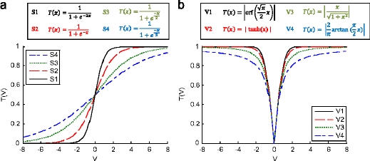
Figure 3.13. S and V transfer function (Mirjalili and Lewis 2013). For a color version of this figure, see www.iste.co.uk/chelouah/optimization.zip
We now know the transfer functions S and V allowing the first module to make the transition from space ℝN to [0,1]N. Now let us move on to the binarization module M2 allowing transition from [0,1]N to BN.
3.6.2. Module M2
The first module transforms a vector ![]() in
in ![]() to a vector
to a vector ![]() in [0,1]N. The second module applies logical rules R on the vector
in [0,1]N. The second module applies logical rules R on the vector ![]() The result creates a binary vector Bi =
The result creates a binary vector Bi = ![]() . The rules R are mathematically defined by [3.21]:
. The rules R are mathematically defined by [3.21]:
In the literature, binary metaheuristics applied to the feature selection (Crawford et al. 2017) mainly use the following rules:
- – the change rate rule R1;
- – the standard rule R2;
- – the 1’s complement rule R3;
- – the statistical rule R4.
3.6.2.1. Change rate rule R1
The rule R1 is the simplest but is somewhat risky because it requires us to define by ourselves. in metaheuristics. a threshold probability or rate of modification TM. Unlike the standard rule R2 which is based on dynamic thresholds defined by T, the rule R1 is static.
For each component ![]() of the binary vector
of the binary vector ![]() will take the value 1 only if the modification rate TM is greater than rand with rand a random value between 0 and 1. The rule R1 is defined by equation [3.22].
will take the value 1 only if the modification rate TM is greater than rand with rand a random value between 0 and 1. The rule R1 is defined by equation [3.22].
This rule has been used in the bABC metaheuristics (Schiezaro and Pedrini 2013) with mixed results. As we specified above, this rule is too “simplistic” because it does not take into account the feedback between the metaheuristics, the objective function and the updating of the positions of the agents in the search space as the standard rule R2 does.
3.6.2.2. Standard rule
The standard rule R2 exploits the dynamism of the S transfer function to provide the value ![]() , making it possible to measure the probability of
, making it possible to measure the probability of ![]() to be 0 or 1.
to be 0 or 1.
This rule will be applied to each bit ![]() of the binary vector Bi =
of the binary vector Bi = ![]() The obtained probability values will be compared to a random value rand ∈ [0,1]. The rule R2 is defined by equations [3.23]:
The obtained probability values will be compared to a random value rand ∈ [0,1]. The rule R2 is defined by equations [3.23]:
This rule has been used in the bDA metaheuristics (Mafarja et al. 2018) and has provided very good results.
The rule R3 that we will see below is a variant of R2.
3.6.2.3. 1’s complement rule R3
The 1’s complement rule R3 is similar to the standard rule R2. There are two differences:
- – the rule R3 is used with V transfer functions while R2 is used with S transfer functions;
- – R3 uses the 1’s complement to calculate the value
 (t) of the binary vector
  .
.
The rule R3 is defined by equation [3.24]:
The rule R3 has been used in the bPSO metaheuristic (Collette and Siarry 2002) by demonstrating the performances of V transfer functions compared to S transfer functions.
The three rules R1, R2 and R3 provide a binary value ![]() from a logical condition. The statistic rule R4 will make it possible to make a choice between three binary values depending on the probability value
from a logical condition. The statistic rule R4 will make it possible to make a choice between three binary values depending on the probability value ![]() and a real value θ.
and a real value θ.
3.6.2.4. Statistic rule R4
As explained above, the statistical rule R4 uses the probability value ![]() and ? to generate three logical conditions. These three logical conditions form a stochastic crossover operation between the values
and ? to generate three logical conditions. These three logical conditions form a stochastic crossover operation between the values ![]() ,
, ![]() and
and ![]() . At the end of this operation,
. At the end of this operation, ![]() will take one of the values
will take one of the values ![]() ,
, ![]() or
or ![]() . The rule R4 is defined by equation [3.25]:
. The rule R4 is defined by equation [3.25]:
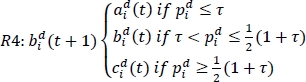
This rule will be used in the bGWO metaheuristic (Emary et al. 2016) below.
We now have all theoretical knowledge and mathematical tools to adapt the GWO to optimization in a binary research space. This adaptation will lead to the bGWO metaheuristic that will provide an acceptable solution in a reasonable time to the problem of feature selection.
3.7. Adaptation of the grey wolf algorithm to feature selection in a binary search space
In this section, we build on the work of Emary et al. on the grey wolf binary optimization approaches for feature selection (Emary et al. 2016). These works propose two binarization algorithms of the GWO algorithm.
The first algorithm will have the same steps as the continuous version GWO until the pack hierarchy update ![]() ,
, ![]() and
and ![]() .
.
On the other hand, the stages of calculating the vectors ![]() ,
, ![]() and
and ![]() will be binarized with the modules M1 and M2. And to get the next grey wolf bit position update
will be binarized with the modules M1 and M2. And to get the next grey wolf bit position update ![]() (t + 1), a statistical logic rule will be used.
(t + 1), a statistical logic rule will be used.
The second algorithm makes it possible to keep almost all steps of the continuous version GWO. Only the update operation of ![]() (t+1) will be binarized with M1 and M2.
(t+1) will be binarized with M1 and M2.
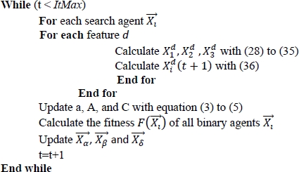
3.7.1. First algorithm bGWO1
In this approach, each bit ![]() (t) of the binary vectors
(t) of the binary vectors ![]() ,
, ![]() and
and ![]() is calculated respectively using equations [3.27]–[3.29], [3.30]–[3.32] and [3.33]–[3.35].
is calculated respectively using equations [3.27]–[3.29], [3.30]–[3.32] and [3.33]–[3.35].
In this approach, the module M1 will use the following S transfer function [3.26]:
The module M2 uses the standard rule R2 and the statistical rule R4 to calculate the next bit position of the grey wolves.
In the following we will implement the modules Ml and M2 on the vector ![]() . The process is the same for vectors
. The process is the same for vectors ![]() and
and ![]() .
.
3.7.1.1. Module M1
In the continuous version GWO version ![]()
![]()
The module M1 uses the value ![]() to measure the remoteness from the position of the prey. Let x =
to measure the remoteness from the position of the prey. Let x = ![]() in the S transfer function [3.27]. The result
in the S transfer function [3.27]. The result ![]() measures the probability of having the value 1 or 0.
measures the probability of having the value 1 or 0.
3.7.1.2. Module M2
The module M2 uses the standard rule [3.28] to obtain the binary value ![]() , and the logic rule [3.29] to obtain the binary value
, and the logic rule [3.29] to obtain the binary value ![]() knowing that
knowing that ![]() is a binary value.
is a binary value.
Vector ![]()
Equations [3.30]–[3.32] and [3.33]–[3.35] apply the modules M1 and M2 in the same way in order to calculate the vectors ![]() and
and ![]() .
.
Vector ![]() 2
2
Vector ![]()
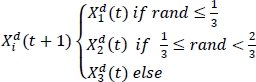
The module M2 ends by calculating the next binary position ![]() with the statistical rule [3.36] by performing a stochastic crossing of
with the statistical rule [3.36] by performing a stochastic crossing of ![]()
![]() with
with ![]() .
.
The first algorithm bGWO1 makes it possible to search for the best binary position of a wolf agent to solve the optimization problem in a binary search space ![]() N with N features. The quality of bGWOI is that it retains the same optimization strategy as GWO while binarizing it thanks to modules M1 and M2. Indeed, these two modules are implemented to calculate the binary positions
N with N features. The quality of bGWOI is that it retains the same optimization strategy as GWO while binarizing it thanks to modules M1 and M2. Indeed, these two modules are implemented to calculate the binary positions ![]() ,
, ![]() and
and ![]() in the surrounding areas created by the hierarchy of the pack and then to calculate the new binary position of the wolf agents of the pack.
in the surrounding areas created by the hierarchy of the pack and then to calculate the new binary position of the wolf agents of the pack.
In the second algorithm, bGWO2 reduces the binarization phases. Only the calculation for updating the positions of wolf agents is binarized.
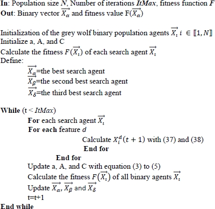
3.7.2. Second algorithm bGWO2
In this second approach, as in the first approach, the module M1 uses the transfer function [3.26] and the standard rule R2 in the module M2.
As we have just explained, in bGWO2, only the update phase of the bit positions is binarized. To do this, each component ![]() will be calculated using the average of
will be calculated using the average of ![]() from the positions
from the positions ![]()
![]() and
and ![]() . Therefore,
. Therefore, ![]() in function tranfers [3.26].
in function tranfers [3.26].
Thus, the module M1 calculates ![]() in [3.37] which makes it possible to evaluate the probability that
in [3.37] which makes it possible to evaluate the probability that ![]() takes the value 1 or 0.
takes the value 1 or 0.
The module M2 calculates the next value of ![]() by using the standard rule R2 in [3.38].
by using the standard rule R2 in [3.38].
The bGWO2 algorithm is more attractive than bGWO1 because only the step of updating the pack positions is binarized. Everything else in the bGWO2 algorithm is identical to GWO.
The pseudocodes of bGWO1 and bGWO2, respectively, provided by Algorithm 2 and Algorithm 3 allow them to be compared to the GWO algorithm and to confirm the consistency of the hunting strategy used in the GWO.
3.7.3. Algorithm 2: first approach of the binary GWO
In: Population size N, Number of iterations ItMax, fitness function F
Out: Binary vector ![]() and fitness value F(
and fitness value F(![]() )
)
Initialization of the grey wolf binary population agents ![]() Initialize a, A, and C
Initialize a, A, and C
Calculate the fitness F(![]() i) of each search agent
i) of each search agent ![]() i
i
Define:
 = the first best search agent
 = the second best search agent
 = the third best search agent
3.7.4. Algorithm 3: second approach of the binary GWO
3.8. Experimental implementation of bGWO1 and bGWO2 and discussion
The wrapper feature selection method was used in Emary et al. (2016) to select the features of 18 datasets from the UCI reference system (Frank and Asuncion 2010). They are compared to known metaheuristics in the literature: genetic algorithm (GA) and PSO.
The wrapper consists of bGWO1 and bGWO2 metaheuristics and the KNN classification algorithm.
Each dataset is divided into three portions: training data, validation data and test data. Only training and validation data are used for feature selection. The test data will be used to test the final classifier with the selected features.
The objective function is composed of the error rate ℰ provided by the validation phase and the number of features D calculated by the sum of the bits equal to 1 in the binary vectors. θ is set at 0.99. Therefore, this is the minimization of the error rate ℰ which is favored.
In order to confirm the repeatability of the experimental results and to test the stability and robustness of the metaheuristics, it is necessary to perform several runs of bGWO1 and bGWO2 on the datasets. NE is the number of runs.
In Emary (2016), the parameters of the experiment are provided by Table 3.2.
Table 3.2. Wrapper parameters
|
Parameters |
Values |
|
Number of wolf agents |
8 |
|
Number of iterations |
70 |
|
NE |
20 |
|
θ |
0.99 |
|
K |
5 |
The complete experimental results are provided by Emary (2016). We described in Table 3.3 the main experimental performance metrics which make it possible to validate the feature selection of the 18 UCI datasets with the bGWO-KNN wrapper.
Table 3.3. Wrapper performance metrics
|
Performance metrics |
Description |
|
The average error rate of the KNN classifier |
Sum of error rates divided by NE. This is an indicator of the quality of the classifier on the selected data subset |
|
Best solution found |
This is the solution that provided the best results on NE runs |
|
Worst solution found |
This is the solution that provided the worst results on NE runs |
|
The average of the solutions over the NE runs of the algorithm |
Sum of the solutions on the NE executions divided by NE. It is a performance indicator of the algorithm. |
|
Standard deviation of the solutions found on the NE runs of the algorithm |
Measures the average variation of the solutions found on the runs. This is an indicator of the stability and robustness of the algorithm |
|
The average size rate of the selected features divided by the feature size N of the data on the number NE of runs of the algorithm |
Sum of features selected D divided by Nx NE during NE runs |
|
The mean Fisher score of the selected data subset |
The Fisher score measures the separability of data by measuring the inter-class and intra-class distances of the selected data subset. The inter-class distances must be as large as possible and the intra-class distances as small as possible |
By analyzing the results provided by Emary et al. (2016) we can see that globally the metaheuristics bGWO1 and bGWO2 are more competitive and efficient than GA and PSO.
3.9. Conclusion
This chapter has revealed another usefulness of population-based metaheuristics in data processing for the benefit of machine learning algorithms. Indeed, metaheuristics are able to solve with very good results the optimization problems of feature selection. Feature selection provides strategic advantages in the training of classifiers by increasing their performance while reducing their complexity.
In addition, we learned to adapt a continuous population-based metaheuristic to optimization in a binary search space. To this end, we have chosen a recent metaheuristic to explain the binarization methods: the grey wolf metaheuristics GWO.
The binarization methods are composed of two modules and they made it possible to create two new metaheuristics for feature selection: bGWO1 and bGWO2.
The experimental results, on 18 datasets from the UCI reference system, demonstrated the superiority of bGWO1 and bGWO2 compared to the bGA and bPSO algorithms.
The performance of bGWO has attracted the attention of several researchers and has led to improvements through hybridization techniques such as bPSOGWO (Al-Tashi et al. 2017). This shows that the room for maneuver for improvements in metaheuristic GWO is extensive.
3.10. References
Afshinmanesh, F., Marandi, A., Rahimi-Kian, A. (2005). A novel binary particle swarm optimization method using artificial immune system. EUROCON 2005 – The International Conference on Computer as a Tool. IEEE, Belgrade.
Al-Tashi, Q., Abdulkadir, S.J., Rais, H.M., Mirjalili, S., Alhussian, H. (2017). Binary optimization using hybrid grey wolf optimization for feature selection. IEEE Access, 7, 39496–39508.
Almomani, A., Alweshah, M., Al Khalayleh, S., Al-Refai, M., Qashi, R. (2019). Metaheuristic algorithms-based feature selection approach for intrusion detection. Machine Learning for Computer and Cyber Security: Principles, Algorithms and Practices, Gupta, B.B., Sheng, Q.Z. (eds). CRC Press, Boca Raton, FL.
Chandrashekar, G. and Sahin, F. (2014). A survey on feature selection methods. Computers & Electrical Engineering, 40(1), 16–28.
Collette, Y. and Siarry, P. (2002). Optimisation Multiobjectif. Eyrolles, Paris.
Crawford, B., Soto, R., Astorga, G., García, J., Castro, C., Paredes, F. (2017). Putting continuous metaheuristics to work in binary search spaces. Hindawi, 2017, 8404231.
Emary, E., Zawbaab, H.M., Hassanien, A.E. (2016). Binary grey wolf optimization approaches for feature selection. Distributed Learning Algorithms for Swarm Robotics, 172, 371–381.
Faris, H., Aljarah, I., Al-Betar, M.A., Mirjalili, S. (2017). Grey wolf optimizer: A review of recent variants and applications. Neural Computing and Applications, 30, 413–435.
Fong, S., Deb, S., Yang, X.S., Li, J. (2014). Feature selection in life science classification: Metaheuristic swarm search. IEEE, IT Professional, 16(4), 24–29.
Frank, A. and Asuncion, A. (2010). UCI Machine Learning Repository [Online]. Available at: http://archive.ics.uci.edu/ml/index.php.
Hodashinsky, I.A. and Sarin, K.S. (2019). Feature selection: Comparative analysis of binary metaheuristics and population based algorithm with adaptive memory. Programming and Computer Software, 45(5), 221–227.
Mafarja, M., Eleyan, D., Abdullah, S., Mirjalili, S. (2017). S-shaped vs. V-shaped transfer functions for ant lion optimization algorithm in feature selection problem. Proceedings of the International Conference on Future Networks and Distributed Systems (ICFNDS ‘17). Association for Computing Machinery, New York.
Mafarja, M., Aljarah, I., Heidari, A.H., Faris, H., Fournier-Viger, P., Li, X., Mirjalili, S. (2018). Binary dragonfly optimization for feature selection using time-varying transfer functions. Knowledge-Based Systems, 161, 185–204.
Mirjalili, S. and Lewis, A. (2013). S-shaped versus V-shaped transfer functions for binary particle swarm optimization. Swarm and Evolutionary Computation, 9, 1–14.
Mirjalili, S., Mirjalili, S.M., Lewis, A. (2014). Grey wolf optimizer. Advances in Engineering Software, 69, 46–61.
Sakr, M.M., Tawfeeq, M.A., El-Sisi, A.B. (2019). Filter versus wrapper feature selection for network intrusion detection system. Ninth International Conference on Intelligent Computing and Information Systems (ICICIS), IEEE, Cairo.
Schiezaro, M. and Pedrini, H. (2013). Data feature selection based on artificial bee colony algorithm. Journal on Image and Video Processing, 2013, 47.
Sharma, M. and Kaur, P. (2021). A comprehensive analysis of nature-inspired meta-heuristic techniques for feature selection problem. Archives of Computational Methods in Engineering, 28, 1103–1127.
Siarry, P. (2014). Métaheuristiques. Eyrolles, Paris.
Vale, Z.A., Ramos, C., Faria, P., Soares, J.P., Canizes, B., Teixeira, J., Khodr, H.M. (2010). Comparison between deterministic and metaheuristic methods applied to ancillary services dispatch. International Conference on Industrial, Engineering and Other Applications of Applied Intelligent Systems. Springer, Córdoba.