
![]()
This chapter details database features that impact the performance of storing and retrieving data within a table. Table performance is partially determined by database characteristics implemented prior to creating tables. For example, the physical storage features implemented when first creating a database and associated tablespaces subsequently influence the performance of tables. Similarly, performance is also impacted by your choice of initial physical features such as table types and data types. Therefore implementing practical database, tablespace, and table creation standards (with performance in mind) forms the foundation for optimizing data availability and scalability.
An Oracle database is comprised of the physical structures used to store, manage, secure, and retrieve data. When first building a database, there are several performance-related features that you can implement at the time of database creation. For example, the initial layout of the datafiles and the type of tablespace management are specified upon creation. Architectural decisions taken at this point often have long-lasting implications.
![]() Tip An Oracle instance is defined to be the memory structures and background processes. Whereas an Oracle database consists of physical files—namely, data files, control files, and online redo log files.
Tip An Oracle instance is defined to be the memory structures and background processes. Whereas an Oracle database consists of physical files—namely, data files, control files, and online redo log files.
As depicted in Figure 1-1, a tablespace is the logical structure that allows you to manage a group of datafiles. Datafiles are the physical datafiles on disk. When configuring tablespaces, there are several features to be aware of that can have far-reaching performance implications, namely locally managed tablespaces and automatic segment storage managed (ASSM) tablespaces. When you reasonably implement these features, you maximize your ability to obtain acceptable future table performance.
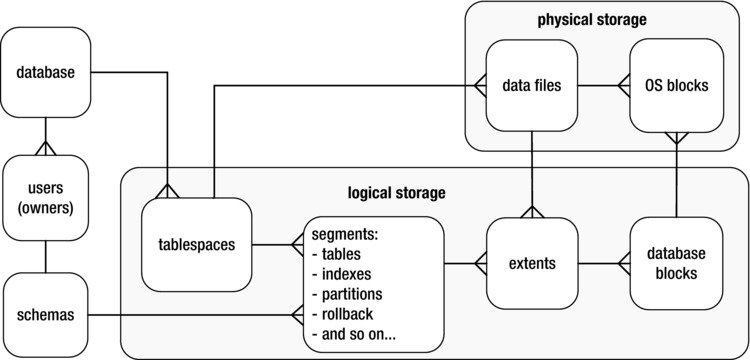
Figure 1-1. Relationships of logical and physical storage
The table is the object that stores data in a database. One measure of database performance is the speed at which an application is able to insert, update, delete, and select data. Therefore it’s appropriate that we begin this book with recipes that provide solutions regarding problems related to table performance.
We start by describing aspects of database and tablespace creation that impact table performance. We next move on to topics such as choosing table types and data types that meet performance-related business requirements. Later topics include managing the physical implementation of tablespace usage. We detail issues such as detecting table fragmentation, dealing with free space under the high-water mark, row migration/chaining, and compressing data. Also described is the Oracle Segment Advisor. This handy tool helps you with automating the detection and resolution of table fragmentation and unused space.
1-1. Building a Database That Maximizes Performance
Problem
You realize when initially creating a database that some features (when enabled) have long-lasting implications for table performance and availability. Specifically, when creating the database, you want to do the following:
- Enforce that every tablespace ever created in the database must be locally managed. Locally managed tablespaces deliver better performance than the obsolete dictionary-managed technology.
- Ensure users are automatically assigned a default permanent tablespace. This guarantees that when users are created they are assigned a default tablespace other than SYSTEM. With the deferred segment feature (more on this later), if a user has the CREATE TABLE privilege, then it is possible for that user to create objects in the SYSTEM tablespace even without having a space quota on the SYSTEM tablespace. This is undesirable. It’s true they won’t be able to insert data into tables without appropriate space quotas, but they can create objects, and thus inadvertently clutter up the SYSTEM tablespace.
- Ensure users are automatically assigned a default temporary tablespace. This guarantees that when users are created they are assigned the correct temporary tablespace when no default is explicitly provided.
Solution
There are two different tools that you can use to create an Oracle database:
- SQL*Plus using the CREATE DATABASE statement
- Database Configuration Assistant (dbca)
These techniques are described in the following subsections.
SQL*Plus
Use a script such as the following to create a database that adheres to reasonable standards that set the foundation for a well-performing database:
CREATE DATABASE O12C
   MAXLOGFILES 16
   MAXLOGMEMBERS 4
   MAXDATAFILES 1024
   MAXINSTANCES 1
   MAXLOGHISTORY 680
   CHARACTER SET AL32UTF8
DATAFILE
'/u01/dbfile/O12C/system01.dbf'
   SIZE 500M REUSE
   EXTENT MANAGEMENT LOCAL
UNDO TABLESPACE undotbs1 DATAFILE
'/u02/dbfile/O12C/undotbs01.dbf'
   SIZE 800M
SYSAUX DATAFILE
'/u01/dbfile/O12C/sysaux01.dbf'
   SIZE 500M
DEFAULT TEMPORARY TABLESPACE TEMP TEMPFILE
'/u02/dbfile/O12C/temp01.dbf'
   SIZE 500M
DEFAULT TABLESPACE USERS DATAFILE
'/u01/dbfile/O12C/users01.dbf'
   SIZE 50M
LOGFILE GROUP 1
        ('/u01/oraredo/O12C/redo01a.rdo',
         '/u02/oraredo/O12C/redo01b.rdo') SIZE 200M,
        GROUP 2
        ('/u01/oraredo/O12C/redo02a.rdo',
         '/u02/oraredo/O12C/redo02b.rdo') SIZE 200M,
        GROUP 3
        ('/u01/oraredo/O12C/redo03a.rdo',
         '/u02/oraredo/O12C/redo03b.rdo') SIZE 200M
USER sys    IDENTIFIED BY f0obar
USER system IDENTIFIED BY f0obar;
The prior CREATE DATABASE script helps establish a good foundation for performance by enabling features such as the following:
- Defines the SYSTEM tablespace as locally managed via the EXTENT MANAGEMENT LOCAL clause; this ensures that all tablespaces ever created in database are locally managed. Starting with Oracle Database 12c, the SYSTEM tablespace is always created as locally managed.
- Defines a default tablespace named USERS for any user created without an explicitly defined default tablespace; this helps prevent users from being assigned the SYSTEM tablespace as the default.
- Defines a default temporary tablespace named TEMP for all users; this helps prevent users from being assigned the SYSTEM tablespace as the default temporary tablespace. Users created with a default temporary tablespace of SYSTEM can have an adverse impact on performance, as this will cause contention for resources in the SYSTEM tablespace.
Solid performance starts with a correctly configured database. The prior recommendations help you create a reliable infrastructure for your table data.
dbca
Oracle’s dbca utility has a graphical interface and a command line mode from which you can configure and create databases. The visual tool is easy to use and has a very intuitive interface. In Linux/Unix environments to use the dbca in graphical mode, ensure you have the proper X software installed, then issue the xhost + command, and make certain your DISPLAY variable is set; for example:
$ xhost +
$ echo $DISPLAY
:0.0

$ xhost +
$ echo $DISPLAY
:0.0
The dbca is invoked from the operating system as follows:
$ dbca
You’ll be presented with a series of screens that allow you to make choices on the configuration. You can choose the “Advanced Mode” option which gives you more control on aspects such as file placement and multiplexing of the online redo logs.
By default, the dbca creates a database with the following characteristics:
- Defines the SYSTEM tablespace as locally managed.
- Defines a default tablespace named USERS for any user created without an explicitly defined default tablespace.
- Defines a default temporary tablespace named TEMP for all users.
Like the SQL*Plus approach, these are all desirable features that provide a good foundation to build applications on.
The dbca utility also allows you to create a database in silent mode, without the graphical component. Using dbca in silent mode with a response file is an efficient way to create databases in a consistent and repeatable manner. This approach also works well when you’re installing on remote servers, which could have a slow network connection or not have the appropriate X software installed.
You can also run the dbca in silent mode with a response file. In some situations, using dbca in graphical mode isn’t feasible. This may be due to slow networks or the unavailability of X software. To create a database, using dbca in silent mode, perform the following steps:
- Locate the dbca.rsp file.
- Make a copy of the dbca.rsp file.
- Modify the copy of the dbca.rsp file for your environment.
- Run the dbca utility in silent mode.
First, navigate to the location in which you copied the Oracle database installation software, and use the find command to locate dbca.rsp:
$ find . -name dbca.rsp
./12.1.0.1/database/response/dbca.rsp
Copy the file so that you’re not modifying the original (in this way, you’ll always have a good, original file):
$ cp dbca.rsp mydb.rsp
Now, edit the mydb.rsp file. Minimally, you need to modify the following parameters: GDBNAME, SID, SYSPASSWORD, SYSTEMPASSWORD, SYSMANPASSWORD, DBSNMPPASSWORD, DATAFILEDESTINATION, STORAGETYPE, CHARACTERSET, and NATIONALCHARACTERSET. Following is an example of modified values in the mydb.rsp file:
[CREATEDATABASE]
GDBNAME = "O12C"
SID = "O12C"
TEMPLATENAME = "General_Purpose.dbc"
SYSPASSWORD = "f00bar"
SYSTEMPASSWORD = "f00bar"
SYSMANPASSWORD = "f00bar"
DBSNMPPASSWORD = "f00bar"
DATAFILEDESTINATION ="/u01/dbfile"
STORAGETYPE="FS"
CHARACTERSET = "AL32UTF8"
NATIONALCHARACTERSET= "UTF8"
Next, run the dbca utility in silent mode, using a response file:
$ dbca -silent -responseFile /home/oracle/orainst/mydb.rsp
You should see output such as
Copying database files
1% complete
...
Creating and starting Oracle instance
...
62% complete
Completing Database Creation
...
100% complete
Look at the log file ... for further details.
If you look in the log files, note that the dbca utility uses the rman utility to restore the data files used for the database. Then, it creates the instance and performs post-installation steps. On a Linux server you should also have an entry in the /etc/oratab file for your new database.
Many DBAs launch dbca and configure databases in the graphical mode, but a few exploit the options available to them using the response file. With effective utilization of the response file, you can consistently automate the database creation process. You can modify the response file to build databases on ASM and even create RAC databases. In addition, you can control just about every aspect of the response file, similar to launching the dbca in graphical mode.
![]() Tip You can view all options of the dbca via the help parameter: dbca -help
Tip You can view all options of the dbca via the help parameter: dbca -help
How It Works
A properly configured and created database will help ensure that your database performs well. It is true that you can modify features after the database is created. However, often a poorly crafted CREATE DATABASE script leads to a permanent handicap on performance. In production database environments, it’s sometimes difficult to get the downtime that might be required to reconfigure an improperly configured database. If possible, think about performance at every step in creating an environment, starting with how you create the database.
When creating a database, you should also consider features that affect maintainability. A sustainable database results in more uptime, which is part of the overall performance equation. The CREATE DATABASE statement in the “Solution” section also factors in the following sustainability features:
- Creates an automatic UNDO tablespace (automatic undo management is enabled by setting the UNDO_MANAGEMENT and UNDO_TABLESPACE initialization parameters); this allows Oracle to automatically manage the rollback segments. This relieves you of having to regularly monitor and tweak.
- Places datafiles in directories that follow standards for the environment; this helps with maintenance and manageability, which results in better long-term availability and thus better performance.
- Sets passwords to non-default values for DBA-related users; this ensures the database is more secure, which in the long run can also affect performance (e.g., if a malcontent hacks into the database and deletes data, then performance will suffer).
- Establishes three groups of online redo logs, with two members each, sized appropriately for the transaction load; the size of the redo log directly affects the rate at which they switch. When redo logs switch too often, this can degrade performance. Keep in mind that when you create a new database that you may not know the appropriate size and will have to adjust this later.
You should take the time to ensure that each database you build adheres to commonly accepted standards that help ensure you start on a firm performance foundation.
If you’ve inherited a database and want to verify the default permanent tablespace setting, use a query such as this:
SELECT *
FROM database_properties
WHERE property_name = 'DEFAULT_PERMANENT_TABLESPACE';
If you need to modify the default permanent tablespace, do so as follows:
SQL> alter database default tablespace users;
To verify the setting of the default temporary tablespace, use this query:
SELECT *
FROM database_properties
WHERE property_name = 'DEFAULT_TEMP_TABLESPACE';
To change the setting of the temporary tablespace, you can do so as follows:
SQL> alter database default temporary tablespace temp;
You can verify the UNDO tablespace settings via this query:
SELECT name, value
FROM v$parameter
WHERE name IN ('undo_management','undo_tablespace'),
If you need to change the undo tablespace, first create a new undo tablespace and then use the ALTER SYSTEM SET UNDO_TABLESPACE statement.
1-2. Creating Tablespaces to Maximize Performance
Problem
You realize that tablespaces are the logical containers for database objects such as tables and indexes. Furthermore, you’re aware that if you don’t specify storage attributes when creating objects, then the tables and indexes automatically inherit the storage characteristics of the tablespaces (that the tables and indexes are created within). Therefore you want to create tablespaces in a manner that maximizes table performance and maintainability.
Solution
We recommend that you create your tablespaces with the locally managed and automatic segment space management features (ASSM) enabled. This is the default behavior starting with Oracle Database 12c:
create tablespace tools
datafile '/u01/dbfile/O12C/tools01.dbf' size 100m;
You can verify that the tablespace was created locally managed and is using ASSM via this query:
select tablespace_name, extent_management, segment_space_management
from dba_tablespaces
where tablespace_name='TOOLS';
Here is some sample output:
TABLESPACE_NAME  EXTENT_MANAGEMENT       SEGMENT_SPACE_MANAGEMENT
---------------- ----------------------- -------------------------
TOOLS            LOCAL                   AUTO
How It Works
To be clear, this recipe discusses two separate desirable tablespace features:
Starting with Oracle Database 12c, all tablespaces are created as locally managed. In prior versions of Oracle you had the choice of either locally managed or dictionary managed. Going forward you should always use locally managed tablespaces.
The tablespace segment space management feature can be set to either AUTO (the default) or MANUAL. Oracle strongly recommends that you use AUTO (referred to as ASSM). This allows Oracle to automatically manage many physical space characteristics that the DBA had to previously manually adjust. In most scenarios, an ASSM managed tablespace will process transactions more efficiently than a MANUAL segment space management enabled tablespace. There are a few corner cases where this may not be true. We recommend that you use ASSM unless you have a proven test case where MANUAL is better.
![]() Note You cannot create the SYSTEM tablespace with the ASSM feature. Also, the ASSM feature is valid only for permanent, locally managed tablespaces.
Note You cannot create the SYSTEM tablespace with the ASSM feature. Also, the ASSM feature is valid only for permanent, locally managed tablespaces.
When creating a tablespace, if you don’t specify a uniform extent size, then Oracle will automatically allocate extents is sizes of 64 KB, 1 MB, 8 MB, and 64 MB. Use the auto-allocation behavior if the objects in the tablespace typically are of varying size. You can explicitly tell Oracle to automatically determine the extent size via the EXTENT MANAGEMENT LOCAL AUTOALLOCATE clause.
You can choose to have the extent size be consistently the same for every extent within the tablespace via the UNIFORM SIZE clause. This example uses a uniform extent size of 128k:
create tablespace tools
  datafile '/u01/dbfile/O12C/tools01.dbf' size 100m
  extent management local uniform size 128k;
If you have a good reason to set the extent size to a uniform size, then by all means do that. However, if you don’t have justification, take the default of AUTOALLOCATE.
You can also specify that a datafile automatically grow when it becomes full. This is set through the AUTOEXTEND ON clause. If you use this feature, we recommend that you set an overall maximum size for the datafile. This will prevent runaway or erroneous SQL from accidentally consuming all available disk space (think about what could happen with a cloud service that automatically adds disk space as required for a database). Here’s an example:
create tablespace tools
  datafile '/u01/dbfile/O12C/tools01.dbf' size 100m
  autoextend on maxsize 10G;
1-3. Matching Table Types to Business Requirements
Problem
You’re new to Oracle and have read about the various table types available. For example, you can choose between heap-organized tables, index-organized tables, and so forth. You want to build a database application and need to decide which table type to use.
Solution
Oracle provides a wide variety of table types. The default table type is heap-organized. For most applications, a heap-organized table is an effective structure for storing and retrieving data. However, there are other table types that you should be aware of, and you should know the situations under which each table type should be implemented. Table 1-1 describes each table type and its appropriate use.
Table 1-1. Oracle Table Types and Typical Uses
Table Type/Feature |
Description |
Benefit/Use |
|---|---|---|
The default Oracle table type and the most commonly used. |
Use this table type unless you have a specific reason to use a different type. |
|
Session private data, stored for the duration of a session or transaction; space is allocated in temporary segments. |
Program needs a temporary table structure to store and modify data. Table data isn’t required after the session terminates. |
|
Index-organized (IOT) |
Data stored in a B-tree index structure sorted by primary key. |
Table is queried mainly on primary key columns; good for range scans, provides fast random access. |
A logical table that consists of separate physical segments. |
Type used with large tables with tens of millions of rows; dramatically affects performance scalability of large tables and indexes. |
|
Tables that use data stored in operating system files outside of the database. |
This type lets you efficiently access data in a file outside of the database (like a CSV or text file). External tables also provide an efficient mechanism for transporting data between databases. |
|
A table that stores the output of a SQL query; periodically refreshed when you want the MV table updated with a current snapshot of the SQL result set. |
Aggregating data for faster reporting or replicating data to offload performance to a reporting database. |
|
A group of tables that share the same data blocks. |
Type used to reduce I/O for tables that are often joined on the same columns. Rarely used. |
|
A table with a column with a data type that is another table. |
Seldom used. |
|
A table with a column with a data type that is an object type. |
Seldom used. |
How It Works
In most scenarios, a heap-organized table is sufficient to meet your requirements. This Oracle table type is a proven structure used in a wide variety of database environments. If you properly design your database (normalized structure) and combine that with the appropriate indexes and constraints, the result should be a well-performing and maintainable system.
Normally most of your tables will be heap-organized. However, if you need to take advantage of a non-heap feature (and are certain of its benefits), then certainly do so. For example, Oracle partitioning is a scalable way to build very large tables and indexes. Materialized views are a solid feature for aggregating and replicating data. Index-organized tables are efficient structures when most of the columns are part of the primary key (like an intersection table in a many-to-many relationship). And so forth.
![]() Caution You shouldn’t choose a table type simply because you think it’s a cool feature that you recently heard about. Sometimes folks read about a feature and decide to implement it without first knowing what the performance benefits or maintenance costs will be. You should first be able to test and prove that a feature has solid performance benefits.
Caution You shouldn’t choose a table type simply because you think it’s a cool feature that you recently heard about. Sometimes folks read about a feature and decide to implement it without first knowing what the performance benefits or maintenance costs will be. You should first be able to test and prove that a feature has solid performance benefits.
1-4. Choosing Table Features for Performance
Problem
When creating tables, you want to implement the appropriate table features that maximize performance, scalability, and maintainability.
Solution
There are several performance and sustainability issues that you should consider when creating tables. Table 1-2 describes features specific to table performance.
Table 1-2. Table Features That Impact Performance
Recommendation |
Reasoning |
|---|---|
Consider setting the physical attribute PCTFREE to a value higher than the default of 10% if the table initially has rows inserted with null values that are later updated with large values. If there are never any updates, considering setting PCTFREE to a lower value. |
As Oracle inserts records into a block, PCTFREE specifies what percentage of the block should be reserved (kept free) for future updates. Appropriately set, can help prevent row migration/chaining, which can impact I/O performance if a large percent of rows in a table are migrated/chained. |
All tables should be created with a primary key (with possibly the exception of tables that store information like logs). |
Enforces a business rule and allows you to uniquely identify each row; ensures that an index is created on primary key column(s), which allows for efficient access to primary key values. |
Consider creating a numeric surrogate key to be the primary key for a table when the real-life primary key is a large character column or multiple columns. |
Makes joins easier (only one column to join) and one single numeric key results in faster joins than large character-based columns or composites. |
Consider using auto-incrementing columns (12c) to populate PK columns. |
Saves having to manually write code and/or maintain triggers and sequences to populate PK and FK columns. However, one possible downside is potential contention with concurrent inserts. |
Create a unique key for the logical business key—a recognizable combination of columns that makes a row unique. |
Enforces a business rule and keeps the data cleaner; allows for efficient retrieval of the logical key columns that may be frequently used in WHERE clauses. If the PK is a surrogate key, there will usually be at least one unique key that identifies the logical business key. |
Define foreign keys where appropriate. |
Enforces a business rule and keeps the data cleaner; helps optimizer choose efficient paths to data. |
Consider creating indexes on foreign key columns. |
Can speed up queries that often join on FK and PK columns and also helps prevent certain locking issues. |
Consider special features such as virtual columns, invisible columns (12c), read-only, parallel, compression, no logging, and so on. |
Features such as parallel DML, compression, or no logging can have a performance impact on reading and writing of data. |
How It Works
The “Solution” section describes aspects of tables that relate to performance. When creating a table, you should also consider features that enhance scalability and availability. Often DBAs and developers don’t think of these features as methods for improving performance. However, building a stable and supportable database goes hand in hand with good performance. Table 1-3 describes best practices features that promote ease of table management.
Table 1-3. Table Features That Impact Scalability and Maintainability
Recommendation |
Reasoning |
|---|---|
Use standards when naming tables, columns, views, constraints, triggers, indexes, and so on. |
Helps document the application and simplifies maintenance. |
Specify a separate tablespace for different schemas. |
Provides some flexibility for different backup and availability requirements. |
Let tables and indexes inherit storage attributes from the tablespaces (especially if you use ASSM created tablespaces). |
Simplifies administration and maintenance. |
Create primary-key constraints out of line (as a table constraint). |
Allows you more flexibility when creating the primary key, especially if you have a situation where the primary key consists of multiple columns. |
Use check constraints where appropriate. |
Enforces a business rule and keeps the data cleaner; use this to enforce fairly small and static lists of values. |
If a column should always have a value, then enforce it with a NOT NULL constraint. |
Enforces a business rule and keeps the data cleaner. |
Create comments for the tables and columns. |
Helps document the application and eases maintenance. |
If you use LOBs in Oracle Database 11g or higher, use the new SecureFiles architecture. |
SecureFiles is the recommended LOB architecture; provides access to features such as compression, encryption, and deduplication. |
1-5. Selecting Data Types Appropriately
Problem
When creating tables, you want to implement appropriate data types so as to maximize performance, scalability, and maintainability.
Solution
There are several performance and sustainability issues that you should consider when determining which data types to use in tables. Table 1-4 describes features specific to performance.
Table 1-4. Data Type Features That Impact Performance
Recommendation |
Reasoning |
|---|---|
If a column always contains numeric data and can be used in numeric computations, then make it a number data type. Keep in mind you may not want to make some columns that only contain digits as numbers (such as U.S. zip code or SSN). |
Enforces a business rule and allows for the greatest flexibility, performance, and consistent results when using Oracle SQL math functions (which may behave differently for a “01” character vs. a 1 number); correct data types prevent unnecessary conversion of data types. |
If you have a business rule that defines the length and precision of a number field, then enforce it—for example, NUMBER(7,2). If you don’t have a business rule, make it NUMBER. |
Enforces a business rule and keeps the data cleaner; numbers with a precision defined won’t unnecessarily store digits beyond the required precision. This can affect the row length, which in turn can have an impact on I/O performance. |
For most character data (even fixed length) use VARCHAR2 (and not CHAR). |
The VARCHAR2 data type is more flexible and space efficient than CHAR. Having said that, you may want to use a fixed length CHAR for some data, such as a country iso-code. |
If you have a business rule that specifies the maximum length of a column, then use that length, as opposed to making all columns VARCHAR2(4000). |
Enforces a business rule and keeps the data cleaner. |
Appropriately use date/time-related data types such as DATE, TIMESTAMP, and INTERVAL. |
Enforces a business rule, ensures that the data is of the appropriate format, and allows for the greatest flexibility and performance when using SQL date functions and date arithmetic. |
Avoid large object (LOB) data types if possible. |
Prevents maintenance issues associated with LOB columns, like unexpected growth, performance issues when copying, and so on. |
![]() Note Prior to Oracle Database 12c the maximum length for a VARCHAR2 and NVARCHAR2 was 4,000, and the maximum length of a RAW column was 2,000. Starting with Oracle Database 12c, these data types have been extended to accommodate a length of 32,767.
Note Prior to Oracle Database 12c the maximum length for a VARCHAR2 and NVARCHAR2 was 4,000, and the maximum length of a RAW column was 2,000. Starting with Oracle Database 12c, these data types have been extended to accommodate a length of 32,767.
How It Works
When creating a table, you must specify the columns names and corresponding data types. As a developer or a DBA, you should understand the appropriate use of each data type. We’ve seen many application issues (performance and accuracy of data) caused by the wrong choice of data type. For instance, if a character string is used when a date data type should have been used, this causes needless conversions and headaches when attempting to do date math and reporting. Compounding the problem, after an incorrect data type is implemented in a production environment, it can be very difficult to modify data types, as this introduces a change that might possibly break existing code. Once you go wrong, it’s extremely tough to recant and backtrack and choose the right course. It’s more likely you will end up with hack upon hack as you attempt to find ways to force the ill-chosen data type to do the job it was never intended to do.
Having said that, Oracle supports the following groups of data types:
- Character
- Numeric
- Date/Time
- RAW
- ROWID
- LOB
![]() Tip The LONG and LONG RAW data types are deprecated and should not be used.
Tip The LONG and LONG RAW data types are deprecated and should not be used.
The data types in the prior bulleted list are briefly discussed in the following subsections.
Character
There are four character data types available in Oracle: VARCHAR2, CHAR, NVARCHAR2, and NCHAR.The VARCHAR2 data type is what you should use in most scenarios to hold character/string data. A VARCHAR2 only allocates space based on the number of characters in the string. If you insert a one-character string into a column defined to be VARCHAR2(30), Oracle will only consume space for the one character.
When you define a VARCHAR2 column, you must specify a length. There are two ways to do this: BYTE and CHAR. BYTE specifies the maximum length of the string in bytes, whereas CHAR specifies the maximum number of characters. For example, to specify a string that contains at the most 30 bytes, you define it as follows:
varchar2(30 byte)
To specify a character string that can contain at most 30 characters, you define it as follows:
varchar2(30 char)
In almost all situations you’re safer specifying the length using CHAR. When working with multibyte character sets, if you specified the length to be VARCHAR2(30 byte), you may not get predictable results, because some characters require more than 1 byte of storage. In contrast, if you specify VARCHAR2(30 char), you can always store 30 characters in the string, regardless of whether some characters require more than 1 byte.
The NVARCHAR2 and NCHAR data types are useful if you have a database that was originally created with a single-byte, fixed-width character set, but sometime later you need to store multibyte character set data in the same database.
![]() Tip Oracle does have another data type named VARCHAR. Oracle currently defines VARCHAR as synonymous with VARCHAR2. Oracle strongly recommends that you use VARCHAR2 (and not VARCHAR), as Oracle’s documentation states that VARCHAR might serve a different purpose in the future.
Tip Oracle does have another data type named VARCHAR. Oracle currently defines VARCHAR as synonymous with VARCHAR2. Oracle strongly recommends that you use VARCHAR2 (and not VARCHAR), as Oracle’s documentation states that VARCHAR might serve a different purpose in the future.
Numeric
Use a numeric data typeto store data that you’ll potentially need to use with mathematic functions, such as SUM, AVG, MAX, and MIN. Never store numeric information in a character data type. When you use a VARCHAR2 to store data that are inherently numeric, you’re introducing future failures into your system. Eventually, you’ll want to report or run calculations on numeric data, and if they’re not a numeric data type, you’ll get unpredictable and often wrong results.
Oracle supports three numeric data types:
- NUMBER
- BINARY_DOUBLE
- BINARY_FLOAT
For most situations, you’ll use the NUMBER data type for any type of number data. Its syntax is
NUMBER(scale, precision)
where scale is the total number of digits, and precision is the number of digits to the right of the decimal point. So, with a number defined as NUMBER(5, 2) you can store values +/–999.99. That’s a total of five digits, with two used for precision to the right of the decimal point.
![]() Tip Oracle allows a maximum of 38 digits for a NUMBER data type. This is almost always sufficient for any type of numeric application.
Tip Oracle allows a maximum of 38 digits for a NUMBER data type. This is almost always sufficient for any type of numeric application.
What sometimes confuses developers and DBAs is that you can create a table with columns defined as INT, INTEGER, REAL, DECIMAL, and so on. These data types are all implemented by Oracle with a NUMBER data type. For example, a column specified as INTEGER is implemented as a NUMBER(38).
The BINARY_DOUBLE and BINARY_FLOAT data types are used for scientific calculations. These map to the DOUBLE and FLOAT Java data types. Unless your application is performing rocket science calculations, then use the NUMBER data type for all your numeric requirements.
![]() Note The BINARY data types can lead to rounding errors that you won't have with NUMBER and also the behavior may vary depending on the operating system and hardware.
Note The BINARY data types can lead to rounding errors that you won't have with NUMBER and also the behavior may vary depending on the operating system and hardware.
Date/Time
When capturing and reporting on date-related information, you should always use a DATE or TIMESTAMP data type (and not VARCHAR2 or NUMBER). Using the correct date-related data type allows you to perform accurate Oracle date calculations and aggregations and dependable sorting for reporting. If you use a VARCHAR2 for a field that contains date information, you are guaranteeing future reporting inconsistencies and needless conversion functions (such as TO_DATE and TO_CHAR).
The DATE data type contains a date component as well as a time component that is granular to the second. If you don’t specify a time component when inserting data, then the time value defaults to midnight (0 hour at the 0 second). If you need to track time at a more granular level than the second, then use TIMESTAMP; otherwise, feel free to use DATE.
The TIMESTAMP data type contains a date component and a time component that is granular to fractions of a second. When you define a TIMESTAMP, you can specify the fractional second precision component. For instance, if you wanted five digits of fractional precision to the right of the decimal point, you would specify that as:
TIMESTAMP(5)
The maximum fractional precision is 9; the default is 6. If you specify 0 fractional precision, then you have the equivalent of the DATE data type.
RAW
The RAW data typeallows you to store binary data in a column. This type of data is sometimes used for storing globally unique identifiers or small amounts of encrypted data. If you need to store large amounts (over 2000 bytes) of binary data then use a BLOB instead.
If you select data from a RAW column, SQL*Plus implicitly applies the built-in RAWTOHEX function to the data retrieved. The data are displayed in hexadecimal format, using characters 0–9 and A–F. When inserting data into a RAW column, the built-in HEXTORAW is implicitly applied.
This is important because if you create an index on a RAW column, the optimizer may ignore the index, as SQL*Plus is implicitly applying functions where the RAW column is referenced in the SQL. A normal index may be of no use, whereas a function-based index using RAWTOHEX may result in a substantial performance improvement.
ROWID
Sometimes when developers/DBAs hear the word ROWID (row identifier), they often think of a pseudocolumn provided with every table row that contains the physical location of the row on disk; that is correct. However, many people do not realize that Oracle supports an actual ROWID data type, meaning that you can create a table with a column defined as the type ROWID.
There are a few practical uses for the ROWID data type. One valid application would be if you’re having problems when trying to enable a referential integrity constraint and want to capture the ROWID of rows that violate a constraint. In this scenario, you could create a table with a column of the type ROWID and store in it the ROWIDs of offending records within the table. This affords you an efficient way to capture and resolve issues with the offending data.
Never be tempted to use a ROWID data type and the associated ROWID of a row within the table for the primary key value. This is because the ROWID of a row in a table can change. For example, an ALTER TABLE...MOVE command will potentially change every ROWID within a table. Normally, the primary key values of rows within a table should never change. For this reason, instead of using ROWID for a primary key value, use a sequence-generated non-meaningful number (or in 12c, use an auto-incrementing column to populate a primary key column).
LOB
Oracle supports storing large amounts of data in a column via a LOB data type. Oracle supports the following types of LOBs:
- CLOB
- NCLOB
- BLOB
- BFILE
If you have textual data that don’t fit within the confines of a VARCHAR2, then you should use a CLOB to store these data. A CLOB is useful for storing large amounts of character data, such as text from articles (blog entries) and log files. An NCLOB is similar to a CLOB but allows for information encoded in the national character set of the database.
BLOBs store large amounts of binary data that usually aren’t meant to be human readable. Typical BLOB data include images, audio, word processing documents, pdf, spread sheets, and video files.
CLOBs, NCLOBs, and BLOBs are known as internal LOBs. This is because they are stored inside the Oracle database. These data types reside within data files associated with the database.
BFILEs are known as external LOBs. BFILE columns store a pointer to a file on the OS that is outside the database. When it’s not feasible to store a large binary file within the database, then use a BFILE. BFILEs don’t participate in database transactions and aren’t covered by Oracle security or backup and recovery. If you need those features, then use a BLOB and not a BFILE.
1-6. Avoiding Extent Allocation Delays When Creating Tables
Problem
You’re installing an application that has thousands of tables and indexes. Each table and index are configured to initially allocate an initial extent of 10 MB. When deploying the installation DDL to your production environment, you want install the database objects as fast as possible. You realize it will take some time to deploy the DDL if each object allocates 10 MB of disk space as it is created. You wonder if you can somehow instruct Oracle to defer the initial extent allocation for each object until data is actually inserted into a table.
Solution
The only way to defer the initial segment generation is to use the Enterprise Edition of Oracle Database 11g R2 or higher. With the Enterprise Edition of Oracle, by default the physical allocation of the extent for a table (and associated indexes) is deferred until a record is first inserted into the table. A small example will help illustrate this concept. First a table is created:
create table emp(
 emp_id number
,first_name varchar2(30)
,last_name varchar2(30));
Now query USER_SEGMENTS and USER_EXTENTS to verify that no physical space has been allocated:
SQL> select count(*) from user_segments where segment_name='EMP';
  COUNT(*)
----------
         0

SQL> select count(*) from user_extents where segment_name='EMP';
  COUNT(*)
----------
         0
Next a record is inserted, and the prior queries are run again:
SQL> insert into emp values(1,'John','Smith'),

1 row created.

SQL> select count(*) from user_segments where segment_name='EMP';
 COUNT(*)
----------
         1

SQL> select count(*) from user_extents where segment_name='EMP';
  COUNT(*)
----------
         1
The prior behavior is quite different from previous versions of Oracle. In prior versions, as soon as you create an object, the segment and associated extent are allocated.
![]() Note Deferred segment creation also applies to partitioned tables and indexes. An extent will not be allocated until the initial record is inserted into a given segment.
Note Deferred segment creation also applies to partitioned tables and indexes. An extent will not be allocated until the initial record is inserted into a given segment.
How It Works
Starting with the Enterprise Edition of Oracle Database 11g R2 (and not any other editions, like the Standard Edition), with non-partitioned heap-organized tables created in locally managed tablespaces, the initial segment creation is deferred until a record is inserted into the table. You need to be aware of Oracle’s deferred segment creation feature for several reasons:
- Allows for a faster installation of applications that have a large number of tables and indexes; this improves installation speed, especially when you have thousands of objects.
- As a DBA, your space usage reports may initially confuse you when you notice that there is no space allocated for objects.
- The creation of the first row will take a slightly longer time than in previous versions (because now Oracle allocates the first extent based on the creation of the first row). For most applications, this performance degradation is not noticeable.
- There may be unforeseen side effects from using this feature (more on this in a few paragraphs).
We realize that to take advantage of this feature the only “solution” is to upgrade to Oracle Database 11g R2 (Enterprise Edition), which is often not an option. However, we felt it was important to discuss this feature because you’ll eventually encounter the aforementioned characteristics.
You can disable the deferred segment creation feature by setting the database initialization parameter DEFERRED_SEGMENT_CREATION to FALSE. The default for this parameter is TRUE.
You can also control the deferred segment creation behavior when you create the table. The CREATE TABLE statement has two clauses: SEGMENT CREATION IMMEDIATE and SEGMENT CREATION DEFERRED—for example:
create table emp(
 emp_id number
,first_name varchar2(30)
,last_name varchar2(30))
segment creation immediate;
It should be noted that there are some potential unforeseen side effects of the deferred segment creation. For example, MOS note 1050193.1 describes the potential for sequences that have been defined to start with the number 1, to actually start with the number 2.
Also, since the deferred segment creation feature is supported only in the Enterprise Edition of Oracle, if you attempt to export objects (that have no segments created yet) and attempt to import into a Standard Edition of Oracle, you may receive an error: ORA-00439: feature not enabled. Potential workarounds include setting ALTER SYSTEM SET DEFERRED_SEGMENT_CREATION=FALSE or creating the table with SEGMENT CREATION IMMEDIATE. See MOS note 1087325.1 for further details with this issue.
![]() Note The COMPATIBLE initialization parameter needs to be 11.2.0.0.0 or greater before using the SEGMENT CREATION DEFERRED clause.
Note The COMPATIBLE initialization parameter needs to be 11.2.0.0.0 or greater before using the SEGMENT CREATION DEFERRED clause.
1-7. Maximizing Data-Loading Speeds
Problem
You’re loading a large amount of data into a table and want to insert new records as quickly as possible.
Solution
First, set the table’s logging attribute to NOLOGGING; this minimizes the generation redo for direct path operations (this feature has no effect on regular DML operations). Then use a direct path loading feature, such as the following:
- INSERT /*+ APPEND */ on queries that use a subquery for determining which records are inserted
- INSERT /*+ APPEND_VALUES */ on queries that use a VALUES clause
- CREATE TABLE...AS SELECT
Here’s an example to illustrate NOLOGGING and direct path loading. First, run the following query to verify the logging status of a table:
select table_name, logging
from user_tables
where table_name = 'EMP';
Here is some sample output:
TABLE_NAME LOG
---------- ---
EMP        YES
The prior output verifies that the table was created with LOGGING enabled (the default). To enable NOLOGGING, use the ALTER TABLE statement as follows:
SQL> alter table emp nologging;
Now that NOLOGGING has been enabled, there should be a minimal amount of redo generated for direct path operations. The following example uses a direct path INSERT statement to load data into the table:
SQL> insert /*+APPEND */ into emp (first_name) select username from all_users;
The prior statement is an efficient method for loading data because direct path operations such as INSERT /*+APPEND */ combined with NOLOGGING generate a minimal amount of redo.
Also, make sure you commit the data loaded via direct path, otherwise you won’t be able to view it as Oracle will throw an ORA-12838 error indicating that direct path loaded data must be committed before it is selected.
![]() Note When you direct path insert into a table, Oracle will insert the new rows above the high-water mark. Even if there is ample space freed up via a DELETE statement, when direct path inserting, Oracle will always load data above the high-water mark. This can result in a table consuming a large amount of disk space but not necessarily containing that much data.
Note When you direct path insert into a table, Oracle will insert the new rows above the high-water mark. Even if there is ample space freed up via a DELETE statement, when direct path inserting, Oracle will always load data above the high-water mark. This can result in a table consuming a large amount of disk space but not necessarily containing that much data.
How It Works
Direct path inserts have two performance advantages over regular insert statements:
- If NOLOGGING is specified, then a minimal amount of redo is generated.
- The buffer cache is bypassed and data is loaded directly into the datafiles. This can significantly improve the loading performance.
The NOLOGGING feature minimizes the generation of redo for direct path operations only. For direct path inserts, the NOLOGGING option can significantly increase the loading speed. One perception is that NOLOGGING eliminates redo generation for the table for all DML operations. That isn’t correct. The NOLOGGING feature never affects redo generation for regular INSERT, UPDATE, MERGE, and DELETE statements.
One downside to reducing redo generation is that you can’t recover the data created via NOLOGGING in the event a failure occurs after the data is loaded (and before you back up the table). If you can tolerate some risk of data loss, then use NOLOGGING but back up the table soon after the data is loaded. If your data is critical, then don’t use NOLOGGING with direct path operations. If your data can be easily recreated, then NOLOGGING is desirable when you’re trying to improve performance of large data loads.
What happens if you have a media failure after you’ve populated a table in NOLOGGING mode (and before you’ve made a backup of the table)? After a restore and recovery operation, it will appear that the table has been restored:
SQL> desc emp;
However, when executing a query that scans every block in the table, an error is thrown.
SQL> select * from emp;
This indicates that there is logical corruption in the datafile:
ORA-01578: ORACLE data block corrupted (file # 4, block # 147)
ORA-01110: data file 4: '/u01/dbfile/O12C/users01.dbf'
ORA-26040: Data block was loaded using the NOLOGGING option
As the prior output indicates, the data in the table is unrecoverable. Use NOLOGGING only in situations where the data isn’t critical or in scenarios where you can back up the data soon after it was created.
![]() Tip If you’re using RMAN to back up your database, you can report on unrecoverable datafiles via the REPORT UNRECOVERABLE command.
Tip If you’re using RMAN to back up your database, you can report on unrecoverable datafiles via the REPORT UNRECOVERABLE command.
There are some quirks of NOLOGGING that need some explanation. You can specify logging characteristics at the database, tablespace, and object levels. If your database has been enabled to force logging, then this overrides any NOLOGGING specified for a table. If you specify a logging clause at the tablespace level, it sets the default logging for any CREATE TABLE statements that don’t explicitly use a logging clause.
You can verify the logging mode of the database as follows:
SQL> select name, log_mode, force_logging from v$database;
The next statement verifies the logging mode of a tablespace:
SQL> select tablespace_name, logging from dba_tablespaces;
And this example verifies the logging mode of a table:
SQL> select owner, table_name, logging from dba_tables where logging = 'NO';
How do you tell whether Oracle logged redo for an operation? One way is to measure the amount of redo generated for an operation with logging enabled vs. operating in NOLOGGING mode. If you have a development environment for testing, you can monitor how often the redo logs switch while the transactions are taking place. Another simple test is to measure how long the operation takes with and without logging. The operation performed in NOLOGGING mode should occur faster because a minimal amount of redo is generated during the load.
1-8. Efficiently Removing Table Data
Problem
You’re experiencing performance issues when deleting data from a table. You want to remove data as efficiently as possible.
Solution
You can use either the TRUNCATE statement or the DELETE statement to remove records from a table. TRUNCATE is usually more efficient but has some side effects that you must be aware of. For example, TRUNCATE is a DDL statement. This means Oracle automatically commits the statement (and the current transaction) after it runs, so there is no way to roll back a TRUNCATE statement. Because a TRUNCATE statement is DDL, you can’t truncate two separate tables as one transaction.
This example uses a TRUNCATE statement to remove all data from a table:
SQL> truncate table emp;
When truncating a table, by default all space is de-allocated for the table except the space defined by the MINEXTENTS table-storage parameter. If you don’t want the TRUNCATE statement to de-allocate the currently allocated extents, then use the REUSE STORAGE clause:
SQL> truncate table emp reuse storage;
You can query the DBA/ALL/USER_EXTENTS views to verify if the extents have been de-allocated (or not)—for example:
SQL> select count(*) from user_extents where segment_name = 'EMP';
It’s also worth mentioning here that the TRUNCATE statement is often used when working with partitioned tables. Especially when archiving obsolete data and therefore no longer need information in a particular partition. For example, the following efficiently removes data from a particular partition without impacting other partitions within the table:
SQL> alter table f_sales truncate partition p_2012;
How It Works
If you need the option of choosing to roll back (instead of committing) when removing data, then you should use the DELETE statement. However, the DELETE statement has the disadvantage that it generates a great deal of undo and redo information. Thus for large tables, a TRUNCATE statement is usually the most efficient way to remove data.
Another characteristic of the TRUNCATE statement is that it sets the high-water mark of a table back to zero. Oracle defines the high-water mark of a table as the boundary between used and unused space in a segment. When you create a table, Oracle allocates a number of extents to the table, defined by the MINEXTENTS table-storage parameter. Each extent contains a number of blocks. Before data are inserted into the table, none of the blocks have been used, and the high-water mark is zero. As data are inserted into a table, and extents are allocated, the high-water mark boundary is raised.
When you use a DELETE statement to remove data from a table, the high-water mark doesn’t change. One advantage of using a TRUNCATE statement and resetting the high-water mark is that full table scan queries search only for rows in blocks below the high-water mark. This can have significant performance implications for queries that perform full table scans.
Another side effect of the TRUNCATE statement is that you can’t truncate a parent table that has a primary key defined that is referenced by an enabled foreign-key constraint in a child table—even if the child table contains zero rows. In this scenario, Oracle will throw this error when attempting to truncate the parent table:
ORA-02266: unique/primary keys in table referenced by enabled foreign keys
Oracle prevents you from truncating the parent table because in a multiuser system, there is a possibility that another session can populate the child table with rows in between the time you truncate the child table and the time you subsequently truncate the parent table. In this situation, you must temporarily disable the child table–referenced foreign-key constraints, issue the TRUNCATE statement, and then re-enable the constraints.
Compare the TRUNCATE behavior to that of the DELETE statement. Oracle does allow you to use the DELETE statement to remove rows from a parent table while the constraints are enabled that reference a child table (assuming there are zero rows in the child table). This is because DELETE generates undo, is read-consistent, and can be rolled back. Table 1-5 summarizes the differences between DELETE and TRUNCATE.
Table 1-5. Comparison of DELETE and TRUNCATE
DELETE |
TRUNCATE |
|
|---|---|---|
Option of committing or rolling back changes |
YES |
NO (DDL always commits transaction after it runs.) |
Generates undo |
YES |
NO |
Resets the table high-water mark to zero |
NO |
YES |
Affected by referenced and enabled foreign-key constraints |
NO |
YES |
Performs well with large amounts of data |
NO |
YES |
If you need to use a DELETE statement, you must issue either a COMMIT or a ROLLBACK to complete the transaction. Committing a DELETE statement makes the data changes permanent:
SQL> delete from emp;
SQL> commit;
![]() Note Other (sometimes not so obvious) ways of committing a transaction include issuing a subsequent DDL statement (which implicitly commits an active transaction for a session) or normally exiting out of the client tool (such as SQL*Plus).
Note Other (sometimes not so obvious) ways of committing a transaction include issuing a subsequent DDL statement (which implicitly commits an active transaction for a session) or normally exiting out of the client tool (such as SQL*Plus).
If you issue a ROLLBACK statement instead of COMMIT, the table contains data as it was before the DELETE was issued.
When working with DML statements, you can confirm the details of a transaction by querying from the V$TRANSACTION view. For example, say that you have just inserted data into a table; before you issue a COMMIT or ROLLBACK, you can view active transaction information for the currently connected session as follows:
SQL> insert into emp values(1, 'John', 'Smith'),
SQL> select xidusn, xidsqn from v$transaction;
    XIDUSN     XIDSQN
---------- ----------
         9        369
SQL> commit;
SQL> select xidusn, xidsqn from v$transaction;
no rows selected
![]() Note Another way to remove data from a table is to drop and re-create the table. However, this means you also have to re-create any indexes, constraints, grants, and triggers that belong to the table. Additionally, when you drop a table, it’s temporarily unavailable until you re-create it and re-issue any required grants. Usually, dropping and re-creating a table is acceptable only in a development or test environment.
Note Another way to remove data from a table is to drop and re-create the table. However, this means you also have to re-create any indexes, constraints, grants, and triggers that belong to the table. Additionally, when you drop a table, it’s temporarily unavailable until you re-create it and re-issue any required grants. Usually, dropping and re-creating a table is acceptable only in a development or test environment.
1-9. Displaying Automated Segment Advisor Advice
Problem
You have a poorly performing query accessing a table. Upon further investigation, you discover the table has only a few rows in it. You wonder why the query is taking so long when there are so few rows. You want to examine the output of Oracle’s Segment Advisor to see if there are any space-related recommendations that might help with performance in this situation.
Solution
Use the Segment Advisor to display information regarding tables that may have space allocated to them (that was once used) but now the space is empty (due to a large number of deleted rows). Tables with large amounts of unused space can cause full table scan queries to perform poorly. This is because Oracle is scanning every block beneath the high-water mark, regardless of whether the blocks contain data.
This solution focuses on accessing the Segment Advisor’s advice via the DBMS_SPACE PL/SQL package. This package retrieves information generated by the Segment Advisor regarding segments that may be candidates for shrinking, moving, or compressing. One simple and effective way to use the DBMS_SPACE package (to obtain Segment Advisor advice) is via a SQL query—for example:
SELECT
 'Segment Advice --------------------------'|| chr(10) ||
 'TABLESPACE_NAME  : ' || tablespace_name   || chr(10) ||
 'SEGMENT_OWNER    : ' || segment_owner     || chr(10) ||
 'SEGMENT_NAME     : ' || segment_name      || chr(10) ||
 'ALLOCATED_SPACE  : ' || allocated_space   || chr(10) ||
 'RECLAIMABLE_SPACE: ' || reclaimable_space || chr(10) ||
 'RECOMMENDATIONS  : ' || recommendations   || chr(10) ||
 'SOLUTION 1       : ' || c1                || chr(10) ||
 'SOLUTION 2       : ' || c2                || chr(10) ||
 'SOLUTION 3       : ' || c3 Advice
FROM
TABLE(dbms_space.asa_recommendations('FALSE', 'FALSE', 'FALSE'));
Here is some sample output:
ADVICE
--------------------------------------------------------------------------------
Segment Advice --------------------------
TABLESPACE_NAME  : USERS
SEGMENT_OWNER    : MV_MAINT
SEGMENT_NAME     : EMP
ALLOCATED_SPACE  : 50331648
RECLAIMABLE_SPACE: 40801189
RECOMMENDATIONS  : Enable row movement of the table MV_MAINT.EMP and perform
 shrink, estimated savings is 40801189 bytes.
SOLUTION 1       : alter table "MV_MAINT"."EMP" shrink space
SOLUTION 2       : alter table "MV_MAINT"."EMP" shrink space COMPACT
SOLUTION 3       : alter table "MV_MAINT"."EMP" enable row movement
In the prior output, the EMP table is a candidate for freeing up space through an operation such as shrinking it or reorganizing the table.
How It Works
In Oracle Database 10g R2 and later, Oracle automatically schedules and runs a Segment Advisor job. This job analyzes segments in the database and stores its findings in internal tables. The output of the Segment Advisor contains findings (issues that may need to be resolved) and recommendations (actions to resolve the findings). Findings from the Segment Advisor are of the following types:
- Segments that are good candidates for shrink operations
- Segments that have significant row migration/chaining
- Segments that might benefit from advanced compression
When viewing the Segment Advisor’s findings and recommendations, it’s important to understand several aspects of this tool. First, the Segment Advisor regularly calculates advice via an automatically scheduled DBMS_SCHEDULER job. You can verify the last time the automatic job ran by querying the DBA_AUTO_SEGADV_SUMMARY view:
select segments_processed, end_time
from dba_auto_segadv_summary
order by end_time;
You can compare the END_TIME date to the current date to determine if the Segment Advisor is running on a regular basis.
![]() Note In addition to automatically generated segment advice, you have the option of manually executing the Segment Advisor to generate advice on specific tablespaces, tables, and indexes (see Recipe 1-10 for details).
Note In addition to automatically generated segment advice, you have the option of manually executing the Segment Advisor to generate advice on specific tablespaces, tables, and indexes (see Recipe 1-10 for details).
When the Segment Advisor executes, it uses the Automatic Workload Repository (AWR) for the source of information for its analysis. For example, the Segment Advisor examines usage and growth statistics in the AWR to generate segment advice. When the Segment Advisor runs, it generates advice and stores the output in internal database tables. The advice and recommendations can be viewed via data dictionary views such as the following:
- DBA_ADVISOR_EXECUTIONS
- DBA_ADVISOR_FINDINGS
- DBA_ADVISOR_OBJECTS
![]() Note The DBA_ADVSIOR_* views are part of the Diagnostics Pack which requires the Enterprise Edition of Oracle and an additional license.
Note The DBA_ADVSIOR_* views are part of the Diagnostics Pack which requires the Enterprise Edition of Oracle and an additional license.
There are three different tools for retrieving the Segment Advisor’s output:
- Executing DBMS_SPACE.ASA_RECOMMENDATIONS
- Manually querying DBA_ADVISOR_* views
- Viewing Enterprise Manager’s graphical screens
In the “Solution” section, we described how to use the DBMS_SPACE.ASA_RECOMMENDATIONS procedure to retrieve the Segment Advisor advice. The ASA_RECOMMENDATIONS output can be modified via three input parameters, which are described in Table 1-6. For example, you can instruct the procedure to show information generated when you have manually executed the Segment Advisor.
Table 1-6. Description of ASA_RECOMMENDATIONS Input Parameters
Parameter |
Meaning |
|---|---|
all_runs |
TRUE instructs the procedure to return findings from all runs, whereas FALSE instructs the procedure to return only the latest run. |
show_manual |
TRUE instructs the procedure to return results from manual executions of the Segment Advisor. FALSE instructs the procedure to return results from the automatic running of the Segment Advisor. |
show_findings |
Shows only the findings and not the recommendations |
You can also directly query the data dictionary views to view the advice of the Segment Advisor. Here’s a query that displays Segment Advisor advice generated within the last day:
select
'Task Name : ' || f.task_name || chr(10) ||
'Start Run Time : ' || TO_CHAR(execution_start, 'dd-mon-yy hh24:mi') || chr (10) ||
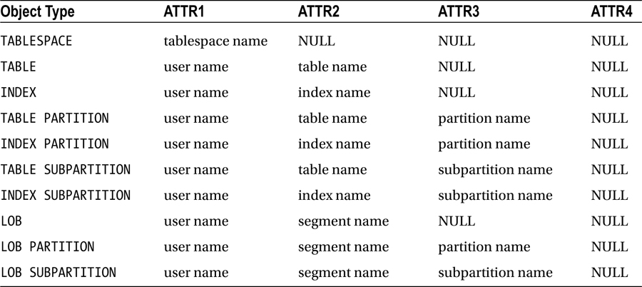
'Segment Name : ' || o.attr2 || chr(10) ||
'Segment Type : ' || o.type || chr(10) ||
'Partition Name : ' || o.attr3 || chr(10) ||
'Message : ' || f.message || chr(10) ||
'More Info : ' || f.more_info || chr(10) ||
'------------------------------------------------------' Advice
FROM dba_advisor_findings f
,dba_advisor_objects o
,dba_advisor_executions e
WHERE o.task_id = f.task_id
AND o.object_id = f.object_id
AND f.task_id = e.task_id
AND e. execution_start > sysdate - 1
AND e.advisor_name = 'Segment Advisor'
ORDER BY f.task_name;
1-10. Manually Generating Segment Advisor Advice
Problem
You have a table that experiences a large amount of updates. Users have reported that queries against this table are performing slower and slower. As part of your analysis you want to manually run the Segment Advisor for this table and see if there are any space related issues such as row migration/chaining, or unused space below the high-water mark.
Solution
You can manually run the Segment Advisor and tell it to specifically analyze all segments in a tablespace or look at a specific object (such as a single table or index). Here are the steps for manually executing the Segment Advisor:
- Create a task.
- Assign an object to the task.
- Set the task parameters.
- Execute the task.
![]() Note The database user executing DBMS_ADVISOR needs the ADVISOR system privilege. This privilege is administered via the GRANT statement.
Note The database user executing DBMS_ADVISOR needs the ADVISOR system privilege. This privilege is administered via the GRANT statement.
The following example encapsulates the four prior steps in a block of PL/SQL. The table being examined is the EMP table and the owner of the table is MV_MAINT:
DECLARE
  my_task_id   number;
  obj_id       number;
  my_task_name varchar2(100);
  my_task_desc varchar2(500);
BEGIN
  my_task_name := 'EMP Advice';
  my_task_desc := 'Manual Segment Advisor Run';
---------
-- Step 1
---------
  dbms_advisor.create_task (
  advisor_name => 'Segment Advisor',
  task_id      => my_task_id,
  task_name    => my_task_name,
  task_desc    => my_task_desc);
---------
-- Step 2
---------
  dbms_advisor.create_object (
  task_name   => my_task_name,
  object_type => 'TABLE',
  attr1       => 'MV_MAINT',
  attr2       => 'EMP',
  attr3       => NULL,
  attr4       => NULL,
  attr5       => NULL,
  object_id   => obj_id);
---------
-- Step 3
---------
  dbms_advisor.set_task_parameter(
  task_name => my_task_name,
  parameter => 'recommend_all',
  value     => 'TRUE'),
---------
-- Step 4
---------
  dbms_advisor.execute_task(my_task_name);
END;
/
Now you can view Segment Advisor advice regarding this table by executing the DBMS_SPACE package and instructing it to pull information from a manual execution of the Segment Advisor (via the input parameters—see Table 1-7 for details)—for example:
SELECT
 'Segment Advice --------------------------'|| chr(10) ||
 'TABLESPACE_NAME  : ' || tablespace_name   || chr(10) ||
 'SEGMENT_OWNER    : ' || segment_owner     || chr(10) ||
 'SEGMENT_NAME     : ' || segment_name      || chr(10) ||
 'ALLOCATED_SPACE  : ' || allocated_space   || chr(10) ||
 'RECLAIMABLE_SPACE: ' || reclaimable_space || chr(10) ||
 'RECOMMENDATIONS  : ' || recommendations   || chr(10) ||
 'SOLUTION 1       : ' || c1                || chr(10) ||
 'SOLUTION 2       : ' || c2                || chr(10) ||
 'SOLUTION 3       : ' || c3 Advice
FROM
TABLE(dbms_space.asa_recommendations('TRUE', 'TRUE', 'FALSE'));
Table 1-7. DBMS_ADVISOR Procedures Applicable for the Segment Advisor
Procedure Name |
Description |
|---|---|
CREATE_TASK |
Creates the Segment Advisor task; specify “Segment Advisor” for the ADVISOR_NAME parameter of CREATE_TASK. Query DBA_ADVISOR_DEFINITIONS for a list of all valid advisors. |
CREATE_OBJECT |
Identifies the target object for the segment advice; Table 1-8 lists valid object types and parameters. |
SET_TASK_PARAMETER |
Specifies the type of advice you want to receive; Table 1-9 lists valid parameters and values. |
EXECUTE_TASK |
Executes the Segment Advisor task |
DELETE_TASK |
Deletes a task |
CANCEL_TASK |
Cancels a currently running task |
You can also retrieve Segment Advisor advice by querying data dictionary views—for example:
SELECT
 'Task Name        : ' || f.task_name  || chr(10) ||
 'Segment Name     : ' || o.attr2      || chr(10) ||
 'Segment Type     : ' || o.type       || chr(10) ||
 'Partition Name   : ' || o.attr3      || chr(10) ||
 'Message          : ' || f.message    || chr(10) ||
 'More Info        : ' || f.more_info TASK_ADVICE
FROM dba_advisor_findings f
    ,dba_advisor_objects  o
WHERE o.task_id = f.task_id
AND o.object_id = f.object_id
AND f.task_name like '&task_name'
ORDER BY f.task_name;
If the table has any space related issues, then the advice output will indicate it as follows:
TASK_ADVICE
--------------------------------------------------------------------------------
Task Name        : EMP Advice
Segment Name     : EMP
Segment Type     : TABLE
Partition Name   :
Message          : The object has chained rows that can be removed by re-org.
More Info        : 22 percent chained rows can be removed by re-org.
How It Works
The DBMS_ADVISOR package is used to manually instruct the Segment Advisor to generate advice for specific tables. This package contains several procedures that perform operations such as creating and executing a task. Table 1-7 lists the procedures relevant to the Segment Advisor.
The Segment Advisor can be invoked with various degrees of granularity. For example, you can generate advice for all objects in a tablespace or advice for a specific table, index, or partition. Table 1-8 lists the object types for which Segment Advisor advice can be obtained via the DBMS_ADVISOR.CREATE_TASK procedure.
Table 1-8. Valid Object Types for the DBMS_ADVISOR.CREATE_TASK Procedure
You can also specify a maximum amount of time that you want the Segment Advisor to run. This is controlled via the SET_TASK_PARAMETER procedure. This procedure also controls the type of advice that is generated. Table 1-9 describes valid inputs for this procedure.
Table 1-9. Input Parameters for the DBMS_ADVISOR.SET_TASK_PARAMETER Procedure
Parameter |
Description |
Valid Values |
|---|---|---|
TIME_LIMIT |
Limit on time (in seconds) for advisor run |
N number of seconds or UNLIMITED (default) |
RECOMMEND_ALL |
Generates advice for all types of advice or just space-related advice |
TRUE (default) for all types of advice, or FALSE to generate only space-related advice |
1-11. Automatically E-mailing Segment Advisor Output
Problem
You realize that the Segment Advisor automatically generates advice and want to automatically e-mail yourself Segment Advisor output.
Solution
First encapsulate the SQL that displays the Segment Advisor output in a shell script—for example:
#!/bin/bash
if [ $# -ne 1 ]; then
  echo "Usage: $0 SID"
  exit 1
fi
# source oracle OS variables
. /etc/oraset $1
#
BOX=`uname -a | awk '{print$2}'`
#
sqlplus -s <<EOF
mv_maint/foo
spo $HOME/bin/log/seg.txt
set lines 80
set pages 100
SELECT
 'Segment Advice --------------------------'|| chr(10) ||
 'TABLESPACE_NAME  : ' || tablespace_name   || chr(10) ||
 'SEGMENT_OWNER    : ' || segment_owner     || chr(10) ||
 'SEGMENT_NAME     : ' || segment_name      || chr(10) ||
 'ALLOCATED_SPACE  : ' || allocated_space   || chr(10) ||
 'RECLAIMABLE_SPACE: ' || reclaimable_space || chr(10) ||
 'RECOMMENDATIONS  : ' || recommendations   || chr(10) ||
 'SOLUTION 1       : ' || c1                || chr(10) ||
 'SOLUTION 2       : ' || c2                || chr(10) ||
 'SOLUTION 3       : ' || c3 Advice
FROM
TABLE(dbms_space.asa_recommendations('FALSE', 'FALSE', 'FALSE'));
EOF
cat $HOME/bin/log/seg.txt | mailx -s "Seg. rpt. on DB: $1 $BOX" [email protected]
exit 0
The prior shell script can be regularly executed from a Linux/Unix utility such as cron. Here is a sample cron entry:
# Segment Advisor report
16 11 * * * /orahome/oracle/bin/seg.bsh DWREP
In this way, you automatically receive segment advice and proactively resolve issues before they become performance problems.
How It Works
The Segment Advisor automatically generates advice on a regular basis. Sometimes it’s handy to proactively send yourself the recommendations. This allows you to periodically review the output and implement suggestions that make sense.
The shell script in the “Solution” section contains a line near the top where the OS variables are established through running an oraset script. This is a custom script that is the equivalent of the oraenv script provided by Oracle. You can use a script to set the OS variables or hard-code the required lines into the script. Calling a script to set the variables is more flexible and maintainable, as it allows you to use as input any database name that appears in the oratab file.
1-12. Rebuilding Rows Spanning Multiple Blocks
Problem
You ran a Segment Advisor report as follows:
SELECT
 'Task Name        : ' || f.task_name  || chr(10) ||
 'Segment Name     : ' || o.attr2      || chr(10) ||
 'Segment Type     : ' || o.type       || chr(10) ||
 'Partition Name   : ' || o.attr3      || chr(10) ||
 'Message          : ' || f.message    || chr(10) ||
 'More Info        : ' || f.more_info TASK_ADVICE
FROM dba_advisor_findings f
    ,dba_advisor_objects  o
WHERE o.task_id   = f.task_id
AND   o.object_id = f.object_id
AND   f.task_name like '&task_name'
ORDER BY f.task_name;
And notice that the output indicates a table with chained rows:
TASK_ADVICE
--------------------------------------------------------------------------------
Task Name        : EMP Advice
Segment Name     : EMP
Segment Type     : TABLE
Partition Name   :
Message          : The object has chained rows that can be removed by re-org.
More Info        : 22%chained rows can be removed by re-org.
You realize that migrated/chained rows leads to higher rates of I/O, and can result in poor performance; therefore you want to eliminate row migration/chaining for this table.
Solution
Row migration/chaining results when there is not enough space within one block to store a row, and therefore Oracle uses more than one block to store the row (more details on this in the “How it Works” section of this recipe). In excess, row migration/chaining can be an issue in that it results in undue I/O when reading a row. There are three basic techniques for resolving row migration/chaining:
- Move the table
- Move individual migrated/chained rows within the table
- Rebuild the table using Data Pump (export/import)
The first two bullets of the prior list are the focus of the “Solution” of this recipe. The Data Pump technique involves exporting the tables, then dropping or renaming the existing tables, and then re-importing the tables from the export file. For details on how to use Data Pump, see the Pro Oracle Database 12c Administration (available from Apress) or Oracle’s Utility Guide available on Oracle’s Technology Network website.
Moving the Table
One method for resolving the row migration/chaining within a table is to use the MOVE statement and rebuild the table and its rows with a lower value of PCTFREE. The idea being that with a lower value of PCTFREE, it will leave more room in the block for the migrated or chained row to fit within (as it’s moved from a block with a high setting of PCTFREE to a block with more room due to the lower setting of PCTFREE).
For example, assume the table was initially built with a PCTFREE value of 40%. This next move operation rebuilds the table with a PCTFREE value of 5%:
SQL> alter table emp move pctfree 5;
However, keep in in mind if you do this, you could make the problem worse, as there will be less room in the block for future updates (which will result in more migrated/chained rows).
![]() Note When you move a table, Oracle requires an exclusive lock on the table; therefore you should perform this operation when there are no active transactions associated with the table being moved.
Note When you move a table, Oracle requires an exclusive lock on the table; therefore you should perform this operation when there are no active transactions associated with the table being moved.
Also, as part of a MOVE operation, all of the rows are assigned a new ROWID. This will invalidate any indexes that are associated with the table. Therefore, as part of the move operation, you should rebuild all indexes associated with the table being moved. You can verify the status of the indexes by interrogating the DBA/ALL/USER_INDEXES view:
select owner, index_name, status
from dba_indexes
where table_name='EMP';
Rebuilding any indexes will make them usable again:
SQL> alter index emp_pk rebuild;
You can verify that row migration and chaining has been resolved (or not) by manually running the Segment Advisor (see Recipe 1-10) or via the ANALYZE TABLE ... COMPUTE STATISTICS command (see the “How it Works” section of this recipe for more details).
Moving Individual Migrated/Chained Rows
You can generate specific ROWIDs for rows that are either migrated or changed via the ANALYZE TABLE ... LIST INTO command. First you must create a table to hold output of the ANALYZE TABLE statement. Oracle provides a script to create a table for you:
SQL> @?/rdbms/admin/utlchn1.sql
The prior script creates a table named CHAINED_ROWS. Now you can run the ANALYZE statement to populate the CHAINED_ROWS table with rows that are migrated and/or chained:
SQL> analyze table emp list chained rows;
Now query the number of rows from the CHAINED_ROWS table:
SQL> select count(*) from chained_rows where table_name='EMP';
The advantage of identifying migrated/chained rows in this manner is that you can potentially fix the migrated/chained rows without impacting the rest of the records in the table by doing the following:
- Create a temporary holding table to store the chained rows.
- Delete the migrated/chained rows from the original table.
- Insert the rows from the temporary table into the original table.
Since this technique has multiple steps, we recommend that you test this first in a non-production environment before you attempt this in a production database. Here’s a short example to demonstrate the prior steps. First create a temporary table that contains the rows in the EMP table that have corresponding records in the CHAINED_ROWS table:
create table temp_emp
as select *
from emp
where rowid in
(select head_rowid from chained_rows where table_name = 'EMP'),
Now delete the records from EMP that have corresponding records in CHAINED_ROWS:
delete from emp
where rowid in
(select head_rowid from chained_rows where table_name = 'EMP'),
Now insert records in the temporary table into the EMP table:
insert into emp select * from temp_emp;
The prior process of moving the migrated/chained rows should clear up any row migration. Now you can delete or truncate the rows from the CHAINED_ROWS table and drop the temporary table.
How do you know if the migrated or chained rows have been fixed? Repeat the process of ANALYZE TABLE ... LIST CHAINED ROWS. If new rows are created in the CHAINED_ROWS table then this means you most likely have chained rows (and not migrated rows) and these can only be resolved by moving the table and adjusting PCTFREE to a lower value or moving the table to a tablespace that has a larger block size (see the “How It Works” section for more details).
UNDERSTANDING THE ORACLE ROWID
Every row in every table has a physical address. The address of a row is determined from a combination of the following:
- Datafile number
- Block number
- Location of the row within the block
- Object number
You can display the address of a row in a table by querying the ROWID pseudo-column—for example:
SQL> select rowid, emp_id from emp;
Here’s some sample output:
ROWID EMP_ID
------------------ ----------
AAAEtQAAEAAAACDAAA 100
AAAEtQAAEAAAACDAAB 101
The ROWID pseudo-column value isn’t physically stored in the database. Oracle calculates its value when you query it. The ROWID contents are displayed as base-64 values that can contain the characters A–Z, a–z, 0–9, +, and /. You can translate the ROWID value into meaningful information via the DBMS_ROWID package. For example, to display the file number, block number, and row number in which a row is stored, issue this statement:
select emp_id
,dbms_rowid.rowid_to_absolute_fno(rowid,schema_name=>'MV_MAINT',object_name=>'EMP') file_num
,dbms_rowid.rowid_block_number(rowid) block_num
,dbms_rowid.rowid_row_number(rowid) row_num
from emp;
Here’s some sample output:
EMP_ID FILE_NUM BLOCK_NUM ROW_NUM
---------- ---------- ---------- ----------
100 4 131 0
101 4 131 1
You can use the ROWID value in the SELECT and WHERE clauses of a SQL statement. In most cases, the ROWID uniquely identifies a row. However, it’s possible to have rows in different tables that are stored in the same cluster and so contain rows with the same ROWID (like with a clustered table).
How It Works
Oracle defines row chaining as a row that is too large to fit within the free space within a block and therefore two or more blocks are required to store the row. Row chaining can occur when:
- A row was initially inserted values that column values that cause the length of the row to be too long to fit within any available block. For an empty block this would roughly be the size of the block minus the space reserved by PCTFREE.
- A row that was initially inserted with column values small enough to fit within one block, but is later updated with values that cause the length of the row to be too long to fit within the free space within the block (the setting of PCTFREE determines what percentage of the block space is reserved for updates).
- A table that has more than 255 columns requires two or more blocks to store it.
Oracle will maintain pointers between the blocks that contain the chained row. This means that anytime the row is read there will be multiple I/O operations. Also updates and deletes may require writing to multiple blocks. If there is a large amount of row chaining this can impact performance. Having said that, if a row is too large to fit within any available block, the only way to fix this is to either reduce the size of the row or increase the size of the block.
For tables with 255 columns or less, you can potentially resolve row chaining by moving the table and at the same time lowering the value of PCTFREE. If that doesn’t resolve the issue, then you could create a tablespace with a larger block size and move the table to that tablespace. Other than those solutions, you won’t be able to avoid row chaining for large rows.
Oracle defines row migration as a row that was initially inserted into a block with values small enough that the row fits within a given free space within a block. The row contains columns that are later updated with larger values (like a column initially is inserted as null and is later updated with a non-null value) which causes the row not to be able to fit within its current block. However, the row is still small enough to fit within the free space of another available block. In this situation, Oracle will move (migrate) this row to another block that has enough space.
With row migration, Oracle maintains a pointer in the original block that points to the block to which the row was migrated. Row migration can impact performance because Oracle has to read/write to multiple blocks any time the row is accessed. Row migration can almost always be resolved by moving the tables as shown in the “Solution” section of this recipe.
1-13. Detecting Row Chaining and Row Migration
Problem
You’re experiencing performance problems selecting from a table. You want to determine if row migration or chaining is a potential issue.
Solution
Here are the options for detecting row migration/chaining:
- Output of the Segment Advisor
- ANALYZE TABLE ... INTO CHAINED_ROWS
- ANALYZE TABLE ... COMPUTE STATISTICS
- Querying V$SYSSTAT
The first two bullets of the prior list have already been discussed in Recipe 1-12. The last two bullets are discussed in the following subsections.
Computing Statistics
A good technique for verifying row migration/chaining is to use the ANALYZE TABLE...COMPUTE STATISTICS statement. Running this for a table results in the CHAINED_CNT column of DBA_TABLES to be populated. For example:
SQL> analyze table emp compute statistics;
Now run this query to give you an idea of what percentage of rows are chained within the table:
select owner, chain_cnt
,round(chain_cnt/num_rows*100,2) chain_pct
,avg_row_len, pct_free
from dba_tables
where table_name = 'EMP';
The CHAIN_CNT contains the sum of both migrated and chained rows that have occurred within the table. If the percentage migrated/chained rows is greater than 15%, then you potentially have an issue.
Querying V$SYSSTAT
Another method for determining if you have an issue with row migration is through querying V$SYSSTAT. After you start your database instance, any time a migrated/chained row is read, the statistic with a value of “table fetch continued row” is incremented. You can view this statistic as follows:
SQL> select name, value from v$sysstat where name = 'table fetch continued row';
Viewed in a vacuum, this statistic is meaningless. If it returned a value of 10,000, you don’t know if that means one migrated row was read 10,000 times or if there are 10,000 tables each with one migrated row that was read once. Furthermore, you don’t know if 10,000 is a bad or good number because you have not compared it to the overall reads from the database since the instance was started.
To get a rough idea if you have an issue with row migration/chaining compare the number reads for migrated/chained rows to the overall number of rows read for your database:
with a as (select sum(value) total_rows_read
           from v$sysstat
           where name like '%table%'
           and name != 'table fetch continued row'),
     b as (select value total_mig_chain_rows
           from v$sysstat where name = 'table fetch continued row')
select a.total_rows_read, b.total_mig_chain_rows,
       b.total_mig_chain_rows/a.total_rows_read pct_rows_mig_or_chained
from a, b;
How It Works
One of the best methods for detecting row chaining or migration is by viewing the output of the Segment Advisor. If you don’t have a license for this tool, then there are other methods such as using the ANALYZE TABLE statement or querying V$SYSSTAT.
If you wanted to analyze all tables in a given schema, you can use SQL to generate SQL:
SQL> select 'analyze table ' || table_name || ' compute statistics;' from user_tables;
The prior script generates the SQL statements required to all tables for the currently connected user. If you have large tables, then keep in mind a may take some time to analyze all of them.
The second approach described in the “Solution” section involves querying V$SYSSTAT. This gives you a more dynamic look at your database. For example, when you check the number of chained rows overall, you don’t necessarily know if they belong to the actively queried part of a large table. Querying V$SYSSTAT helps in this regard because it’s measuring what’s currently transacting in your database.
1-14. Differentiating Between Row Migration and Row Chaining
Problem
You want to determine if you have either row migration or row chaining. This will affect your strategy for resolving the problem. For example, if the issue is row chaining, which is caused by very long records that can’t fit within the given free space in a block, there isn’t much you can do about this. However, row migration might potentially be fixed by moving the table.
Solution
There are three basic techniques for differentiating between row chaining and row migration:
- Re-organizing the table (like moving it) will always fix row migration. It may or may not fix row chaining. So to differentiate between row migration and row chaining, re-organize the table and then compute statistics after the move and anything still showing up in the CHAIN_CNT column is a chained row that couldn’t be resolved by moving the table. Consider modifying the value of PCTFREE to a lower value when you execute the move operation.
- Analyzing the table and recording the ROWIDs in a CHAINED_ROWS table, and then move the individual rows based on the ROWIDs of the migrated/chained rows. Repeat the process, and any new rows populating the CHAINED_ROWS table are chained.
- Calculate the length of each row. If the length of the row is greater than the free space available in an empty block, then most likely the issue is row chaining. If the length of the row is less than the amount of free space within a block size, then the issue is most likely row migration.
The first two bullets have already been discussed in Recipe 1-12. For the last bullet, you can manually calculate the length of a row by summing the lengths of all columns, for example:
SELECT NVL(vsize(emp_id),0) + NVL(vsize(first_name),0) + NVL(vsize(last_name),0)
FROM emp;
Rows that have a greater length than the available free space within an empty block are most likely chained and not migrated.
How It Works
Manually calculating the row length is by far the most accurate method to determine whether you have an issue with row chaining or row migration. If a row’s size approaches the amount of free space within a block, then there may be no way to prevent the row from becoming chained. If the row size is much smaller than the amount of free space within a block, then it is most likely migrated and this issue can be resolved by moving the table (see Recipe 1-12).
![]() Tip Consider using Oracle's compression options to maximize the number of rows per block (see Recipes 1-20 and 1-21 for details).
Tip Consider using Oracle's compression options to maximize the number of rows per block (see Recipes 1-20 and 1-21 for details).
1-15. Proactively Preventing Row Migration/Chaining
Problem
You’ve noticed that a table has often experienced row migration and/or chaining. You want to proactively prevent this issue.
Solution
The amount of free space reserved in a block is determined by the table’s storage parameter of PCTFREE. The default value of PCTFREE is 10, meaning 10% of the block is reserved space to be used for updates that result in more space usage within the row’s current block. If you have a table that has columns that are initially inserted with small and/or null values and later updated to contain large values, then consider setting PCTFREE to a higher value, such as 40%. This will help prevent the row migration. However, keep in mind that a higher value of PCTFREE can result in increased row chaining.
It may help to calculate the average row length after an insert and then do a typical update to the row and again calculate its length. This will give an idea of how much a row will grow (see Recipe 1-14 for details on computing the row length.
If you have a table that is never updated after rows are inserted, then consider setting PCTFREE to 0. This will result in the maximum number of rows per block, which can lead to fewer disk reads (and thus better performance) when retrieving data.
How It Works
You can view the setting for PCTFREE by querying the DBA/ALL/USER_TABLES view—for example:
SQL> select table_name, pct_free from user_tables;
Moving a table almost always fixes migrated rows. The move operation removes each record from the block and re-inserts the record into a new block. For migrated rows, the old chained rows are deleted and rebuilt as one physical row within the block.
Chained rows can only be fixed if the length of the chained row is less than what is free within an empty block. If you have a chained row greater than the amount of free space, then consider setting PCTFREE to a lower value and moving the table or consider creating a tablespace with a larger block size.
1-16. Detecting Unused Space in a Table
Problem
You’re querying a table that has no rows in it, and yet it takes several minutes for the row count to come back as zero. You know from experience that this could be an issue with vacant space within the table. The idea being that a table that initially had many rows in it was subsequently deleted from and this leaves unused space beneath the so called the high-water mark. Subsequent operations such as full table scans can take a long time because Oracle is searching the blocks that initially had data but now do not. Therefore, you want to determine if you have unused space in the table.
Solution
You can detect tables with high-water mark issues by selecting from DBA/ALL/USER_EXTENTS views. If a table has a large number of extents allocated to it but has zero rows, that’s an indication that an extensive amount of data have been deleted from the table; for example:
SQL> select count(*) from user_extents where segment_name='EMP';

  COUNT(*)
----------
        44
Now, inspect the number of rows in the table:
SQL> select count(*) from emp;

  COUNT(*)
----------
         0
The prior table most likely has had data inserted into it, which resulted in extents being allocated. And, subsequently, data were deleted, and the extents remained.
Similarly you can count the number of rows and compare it to the number of blocks allocated to the table. For example:
SQL> select blocks from user_segments where segment_name='EMP';

    BLOCKS
----------
      1024
If the number of blocks is high, but the row count is low, then you most likely have free space beneath the high-water mark.
How It Works
Oracle defines the high-water mark of a table as the boundary between used and unused space in a segment. Also, when you create a table, Oracle allocates a number of extents to the table, defined by the MINEXTENTS table-storage parameter. Each extent contains a number of blocks. Before data are inserted into the table, none of the blocks have been used, and the high-water mark is 0. As data are inserted into a table, and extents are allocated, the high-water mark boundary is raised. A DELETE statement doesn’t reset the high-water mark, thus leaving unused space within the table.
You need to be aware of a couple of performance-related issues regarding the high-water mark:
- SQL query full-table scans
- Direct-path load-space usage
Oracle sometimes needs to scan every block of a table (under the high-water mark) when performing a query. This is known as a full-table scan. If a significant amount of data have been deleted from a table, a full-table scan can take a long time to complete, even for a table with zero rows.
Also, when doing direct-path loads, Oracle inserts data above the high-water mark line. Potentially, you can end up with a large amount of unused space in a table that is regularly deleted from and that is also loaded via a direct-path mechanism.
Besides the technique in the solution section, there are several other ways to detect unused free space below the high-water mark:
- Autotrace tool
- DBMS_SPACE package
- Segment Advisor
See Recipe 1-17 for details on using tracing and Recipe 1-18 for details on using the DBMS_SPACE package. See Recipe 1-10 for details on how to manually run the Segment Advisor.
1-17. Tracing to Detect Space Below the High-Water Mark
Problem
You ran through the steps of Recipe 1-16 and believe you have an issue with unused space beneath the high-water mark for a table. You want to further verify the results by inspecting the output of the Autotrace tool.
You can run this simple test to detect whether you have an issue with unused space below the high-water mark:
- SQL> set autotrace trace statistics
- Run the query that performs the full-table scan.
- Compare the number of rows processed with the number of blocks read from memory.
If the number of rows processed is low but the number of blocks read from memory is high, you may have an issue with the number of free blocks below the high-water mark. Here is a simple example to illustrate this technique:
SQL> set autotrace trace statistics
The next query generates a full-table scan on the INV table:
SQL> select * from inv;
Here is a snippet of the output from AUTOTRACE:
no rows selected

Statistics
----------------------------------------------------------
          4  recursive calls
          0  db block gets
       7371  consistent gets
The number of rows returned is zero, yet there are 7,371 consistent gets (number of blocks read from buffer cache), indicating free space beneath the high-water mark.
Next, truncate the table, and run the query again:
SQL> truncate table inv;
SQL> select * from inv;
Here is a partial listing from the output of AUTOTRACE:
no rows selected

Statistics
----------------------------------------------------------
          6  recursive calls
          0  db block gets
         12  consistent gets
Note that the number of memory accesses are now quite small.
How It Works
Any user granted the PLUSTRACE role can use the Autotrace utility. This tool is available through SQL*Plus and provides details regarding the execution plan and statistics of a successful SELECT, INSERT, UPDATE, DELETE statement. The statistics are recorded internally by Oracle and provide details on the system resources a SQL statement consumes. The consistent gets statistic gives you an indication of how many blocks are read from memory for the given SQL statement. If you have a high consistent gets number and a low row count, then you most likely have an issue with free space under the high-water mark.
1-18. Using DBMS_SPACE to Detect Space Below the High-Water Mark
Problem
You’ve detected evidence of unused space below the high-water mark via tracing (Recipe 1-17). You want to confirm your results via the DBMS_SPACE package.
Solution
Here is an anonymous block of PL/SQL that you can call from SQL*Plus that uses the DBMS_SPACE package to detect free space beneath the high-water mark:
set serverout on size 1000000
declare
   p_fs1_bytes number;
   p_fs2_bytes number;
   p_fs3_bytes number;
   p_fs4_bytes number;
   p_fs1_blocks number;
   p_fs2_blocks number;
   p_fs3_blocks number;
   p_fs4_blocks number;
   p_full_bytes number;
   p_full_blocks number;
   p_unformatted_bytes number;
   p_unformatted_blocks number;
begin
   dbms_space.space_usage(
      segment_owner      => user,
      segment_name       => 'EMP',
      segment_type       => 'TABLE',
      fs1_bytes          => p_fs1_bytes,
      fs1_blocks         => p_fs1_blocks,
      fs2_bytes          => p_fs2_bytes,
      fs2_blocks         => p_fs2_blocks,
      fs3_bytes          => p_fs3_bytes,
      fs3_blocks         => p_fs3_blocks,
      fs4_bytes          => p_fs4_bytes,
      fs4_blocks         => p_fs4_blocks,
      full_bytes         => p_full_bytes,
      full_blocks        => p_full_blocks,
      unformatted_blocks => p_unformatted_blocks,
      unformatted_bytes  => p_unformatted_bytes
   );
   dbms_output.put_line('FS1: blocks = '||p_fs1_blocks);
   dbms_output.put_line('FS2: blocks = '||p_fs2_blocks);
   dbms_output.put_line('FS3: blocks = '||p_fs3_blocks);
   dbms_output.put_line('FS4: blocks = '||p_fs4_blocks);
   dbms_output.put_line('Full blocks = '||p_full_blocks);
end;
/
In this scenario, you want to check the EMP table for free space below the high-water mark. Here is the output of the previous PL/SQL:
FS1: blocks = 0
FS2: blocks = 0
FS3: blocks = 0
FS4: blocks = 3646
Full blocks = 0
In the prior output the FS1 parameter shows that 0 blocks have 0% to 25% free space. The FS2 parameter shows that 0 blocks have 25% to 50% free space. The FS3 parameter shows that 0 blocks have 50% to 75% free space. The FS4 parameter shows there are 3,646 blocks with 75% to 100% free space. Finally, there are 0 full blocks. Because there are no full blocks, and a large number of blocks are mostly empty, you can deduce that free space exists below the high-water mark.
How It Works
The SPACE_USAGE procedure of the DBMS_SPACE package provides you with an alternative method for confirming that you have free space below the high-water mark. This procedure can only be used on tables created within tablespaces create using Automatic Space Segment Management (see Recipe 1-2 for details). See the Oracle PL/SQL Packages and Types Reference guide for more details on how to use this procedure.
1-19. Freeing Unused Table Space
Problem
You’ve analyzed the output of the Segment Advisor and have identified a table that has a large amount of free space below the high-water mark. You want to free up the unused space to improve the performance queries that perform full table scans of the table.
Solution
Do the following to shrink space and re-adjust the high-water mark for a table:
- Enable row movement for the table.
- Use the ALTER TABLE...SHRINK SPACE statement to free up unused space.
![]() Note The shrink table feature requires that the table’s tablespace use automatic space segment management. See Recipe 1-2 for details on how to create an ASSM-enabled tablespace.
Note The shrink table feature requires that the table’s tablespace use automatic space segment management. See Recipe 1-2 for details on how to create an ASSM-enabled tablespace.
When you shrink a table, this requires that rows (if any) be moved which requires that row movement be enabled:
SQL> alter table emp enable row movement;
Next the table shrink operation is executed via an ALTER TABLE statement:
SQL> alter table emp shrink space;
You can also shrink the space associated with any index segments via the CASCADE clause:
SQL> alter table emp shrink space cascade;
How It Works
When you shrink a table, Oracle re-organizes the blocks in a manner that consumes the least amount of space. Oracle also re-adjusts the table’s high-water mark. This has performance implications for queries that result in full table scans. During a full table scan, Oracle will inspect every block below the high-water mark to check it for data that might satisfy the result of a query. If you notice that it takes a long time for a query to return results when there aren’t many rows in the table, this may be an indication that there are many unused blocks (because data was deleted) below the high-water mark.
You can also instruct Oracle to not re-adjust the high-water mark when shrinking a table. This is done via the COMPACT clause—for example:
SQL> alter table emp shrink space compact;
When you use COMPACT, Oracle defragments the table but doesn’t alter the high-water mark. You will need to use the ALTER TABLE...SHRINK SPACE statement to reset the high-water mark. You might want to do this because you’re concerned about the time it takes to defragment and adjust the high-water mark. This allows you to shrink a table in two shorter steps instead of one longer operation.
When you enable row movement for a table, this allows Oracle modify the ROWIDs for any records that need to be moved. This means that Oracle must also maintain indexes that reference those ROWIDs. So just keep in mind that the performance of a table shrink will correspond to the number of rows that need to be moved and indexes that must be updated.
Besides the technique shown in the Solution section, there are two other techniques you can use to free up space beneath the high water mark:
- Truncate the table.
- Move the table.
- Use Data Pump to export the table, drop the table, and then import the table.
Of course, only use TRUNCATE if you want to permanently remove all data from a table. Truncating a table may be acceptable if the table already has zero rows in it.
You can also lower the high water-mark by moving a table. For example:
SQL> alter table emp move;
If you move a table, ensure that you also rebuild any associated indexes, as the move operation will change the ROWIDs of the table rows and invalidate any indexes.
The Data Pump technique involves exporting the tables and then dropping or renaming the existing tables, and then re-importing the tables from the export file. For details on how to use Data Pump, see the Pro Oracle Database 12c Administration (available from Apress) or Oracle’s Utility Guide available on Oracle’s Technology Network website.
1-20. Compressing Data for Direct Path Loading
Problem
You’re using the Enterprise Edition of Oracle and are working with a decision support system (DSS)-type database and you want to improve the performance of an associated reporting application. This environment contains large tables that are loaded once and then frequently subjected to full table scans. You want to compress data as it is loaded because this will compact the data into fewer database blocks and thus will require less I/O for subsequent reads from the table. Because fewer blocks need to be read for compressed data, this will improve data retrieval performance.
Solution
Use Oracle’s basic compression feature to compress direct path–loaded data into a heap-organized table. Basic compression is enabled as follows:
- Use the ROW STORE COMPRESS clause to enable compression either when creating, altering, or moving an existing table.
- Load data via a direct path mechanism such as CREATE TABLE...AS SELECT or INSERT /*+ APPEND */.
![]() Note Prior to Oracle Database 11g R2, basic compression was referred to as DSS compression and enabled via the COMPRESS FOR DIRECT_LOAD OPERATION clause. In 11g R2, this changed to COMPRESS BASIC. In 12c this has now changed to ROW STORE COMPRESS.
Note Prior to Oracle Database 11g R2, basic compression was referred to as DSS compression and enabled via the COMPRESS FOR DIRECT_LOAD OPERATION clause. In 11g R2, this changed to COMPRESS BASIC. In 12c this has now changed to ROW STORE COMPRESS.
Here’s an example that uses the CREATE TABLE...AS SELECT statement to create a basic compression-enabled table and direct path–load the data:
create table regs_dss
compress
as select reg_id, reg_name
from regs;
The prior statement creates a table with compressed data in it. Any subsequent direct path load operations will also load the data in a compressed format.
![]() Tip The following clauses are synonymous: COMPRESS, COMPRESS BASIC, ROW STORE COMPRESS, or ROW STORE COMPRESS BASIC.
Tip The following clauses are synonymous: COMPRESS, COMPRESS BASIC, ROW STORE COMPRESS, or ROW STORE COMPRESS BASIC.
You can verify that compression has been enabled for a table by querying the appropriate DBA/ALL/USER_TABLES view. This example assumes that you’re connected to the database as the owner of the table:
select table_name, compression, compress_for
from user_tables
where table_name='REGS_DSS';
Here is some sample output:
TABLE_NAME                     COMPRESS COMPRESS_FOR
------------------------------ -------- ------------
REGS_DSS                       ENABLED  BASIC
The prior output shows that compression has been enabled in the basic mode for this table. If you’re working with a table has that already been created, then you can alter its basic compression characteristics with the ALTER TABLE statement—for example:
SQL> alter table regs_dss compress;
When you alter a table to enable basic compression, this does not affect any data currently existing in the table; rather, it only compresses subsequent direct path data load operations.
If you want to enable basic compression for data in an existing table, use the MOVE COMPRESS clause:
SQL> alter table regs_dss move compress;
Keep in mind that when you move a table, all of the associated indexes are invalidated. You’ll have to rebuild any indexes associated with the moved table.
If you have enabled basic compression for a table, you can disable it via the NOCOMPRESS clause—for example:
SQL> alter table regs_dss nocompress;
When you alter a table to disable basic compression, this does not uncompress existing data within the table. Rather this operation instructs Oracle to not compress data for subsequent direct path operations. If you need to uncompress existing compressed data, then use the MOVE NOCOMPRESS clause:
SQL> alter table regs_dss move nocompress;
How It Works
The basic compression feature is available at no extra cost with the Oracle Enterprise Edition. Any heap-organized table that has been created or altered to use basic compression will be a candidate for data loaded in a compressed format for subsequent direct path load operations. There is some additional CPU overhead associated with compressing the data, but you may find in many circumstances that this overhead is offset by performance gains due to less I/O.
From a performance perspective, the main advantage to using basic compression is that once the data is loaded as compressed, any subsequent I/O operations will use fewer resources because there are fewer blocks required to read and write data. You will need to test the performance benefits for your environment. In general, tables that hold large amounts of character data are candidates for basic compression—especially in scenarios where data is direct path loaded once, and thereafter selected from many times.
Keep in mind that Oracle’s basic compression feature has no effect on regular DML statements such as INSERT, UPDATE, MERGE, and DELETE. If you require compression to occur on all DML statements, then consider using advanced compression (see Recipe 1-16 for details).
You can also specify basic compression at the partition and tablespace level. Any table created within a tablespace created with the COMPRESS clause will have basic compression enabled by default. Here’s an example of creating a tablespace with the COMPRESS clause:
CREATE TABLESPACE comp_data
  DATAFILE '/u01/dbfile/O12C/comp_data01.dbf'
  SIZE 500M
  EXTENT MANAGEMENT LOCAL
  UNIFORM SIZE 512K
  SEGMENT SPACE MANAGEMENT AUTO
  DEFAULT COMPRESS;
You can also alter an existing tablespace to set the default degree of compression:
SQL> alter tablespace comp_data default compress;
Run this query to verify that basic compression for a tablespace is enabled:
select tablespace_name, def_tab_compression, compress_for
from dba_tablespaces
where tablespace_name = 'COMP_DATA';
![]() Tip You cannot drop a column from a table created with basic compression enabled. However, you can mark a column as unused.
Tip You cannot drop a column from a table created with basic compression enabled. However, you can mark a column as unused.
1-21. Compressing Data for All DML
Problem
You’re in an OLTP environment and have noticed that there is a great deal of disk I/O occurring when reading data from a table. You wonder if you can increase I/O performance by compressing the data within the table. The idea is that compressed table data will consume less physical storage and thus require less I/O to read from disk.
Solution
Use the ROW STORE COMPRESS ADVANCED clause when creating a table to enable data compression when using regular DML statements to manipulate data. This example creates advanced compression–enabled table:
create table regs
(reg_id   number
,reg_name varchar2(2000)
) row store compress advanced;
![]() Note Prior to Oracle Database 11g R2, advanced table compression was enabled using the COMPRESS FOR ALL OPERATIONS clause. In Oracle Database 11g R2, advanced table compression was enabled with COMPRESS FOR OLTP. In Oracle Database 12c, this changed to ROW STORE COMPRESS ADVANCED.
Note Prior to Oracle Database 11g R2, advanced table compression was enabled using the COMPRESS FOR ALL OPERATIONS clause. In Oracle Database 11g R2, advanced table compression was enabled with COMPRESS FOR OLTP. In Oracle Database 12c, this changed to ROW STORE COMPRESS ADVANCED.
You can verify that compression has been enabled for a table by querying the appropriate DBA/ALL/USER_TABLES view. This example assumes that you’re connected to the database as the owner of the table:
select table_name, compression, compress_for
from user_tables
where table_name='REGS';
If you’ve already created the table, you can use the ALTER TABLE statement to enable compression on an existing table—for example:
SQL> alter table regs row store compress advanced;
When you alter a table’s compression mode, it doesn’t impact any of the data currently within the table. Subsequent DML statements will result in data stored in a compressed fashion.
If you want to enable advanced compression for data in an existing table, use the MOVE ROW STORE COMPRESS ADVANCED clause:
SQL> alter table regs move row store compress advanced;
Keep in mind that when you move a table, all of the associated indexes are invalidated. You’ll have to rebuild any indexes associated with the moved table.
If you have enabled advanced compression for a table, you can disable it via the NOCOMPRESS clause—for example:
SQL> alter table regs nocompress;
When you alter a table to disable advanced compression, this does not uncompress existing data within the table. Rather, this operation instructs Oracle to not compress data for subsequent DML operations.
How It Works
The ROW STORE COMPRESS ADVANCED clause enables compression for all DML operations. The advanced compression doesn’t immediately compress data as it is inserted or updated in a table. Rather the compression occurs in a batch mode when the degree of change within the block reaches a certain threshold. When the threshold is reached, all of the uncompressed rows are compressed at the same time. The threshold at which compression occurs is determined by an internal algorithm (over which you have no control).
You can also specify advanced compression at the tablespace level. Any table created in an advanced compression–enabled tablespace will by default inherit this compression setting. Here’s an example of tablespace creation script specifying advanced compression:
CREATE TABLESPACE comp_data
  DATAFILE '/u01/dbfile/O12C/comp_data01.dbf'
  SIZE 500M
  EXTENT MANAGEMENT LOCAL
  UNIFORM SIZE 1M
  SEGMENT SPACE MANAGEMENT AUTO
  DEFAULT ROW STORE COMPRESS ADVANCED;
You can also alter an existing tablespace to set the default degree of compression:
SQL> alter tablespace comp_data default row store compress advanced;
You can verify the default compression characteristics with this query:
select tablespace_name, def_tab_compression, compress_for
from dba_tablespaces
where tablespace_name = 'COMP_DATA';
1-22. Compressing Data at the Column Level
Problem
You’re using the Oracle Exadata product and you want to efficiently compress data. You have determined that compressed data will result in much more efficient I/O operations, especially when reading data from disk. The idea is that compressed data will result in much fewer blocks read for SELECT statements.
Solution
To enable column compression (Oracle refers to this feature as hybrid columnar compression), when creating a table, use either the COLUMN STORE COMPRESS FOR QUERY or the COLUMN STORE COMPRESS FOR ARCHIVE clause—for example:
create table emp(
 emp_id number
,first_name varchar2(30)
,last_name varchar2(30))
column store compress for query;
You can also specify a level of compression of either LOW or HIGH:
create table emp(
 emp_id number
,first_name varchar2(30)
,last_name varchar2(30))
column store compress for query high;
The default level of compression for QUERY is HIGH, and the default level of compression for ARCHIVE is LOW. You can validate the level of compression enabled via this query:
select table_name, compression, compress_for
from user_tables
where table_name='EMP';
If you attempt to use hybrid columnar compression in an environment other than Exadata, you’ll receive the following error:
ORA-64307:  Exadata Hybrid Columnar Compression is not supported for
tablespaces on this storage type
How It Works
Exadata is Oracle’s high-performance database machine. It is designed to deliver high performance for both data warehouse and OLTP databases. Exadata storage supports hybrid columnar compression and is available starting with Oracle Database 11g R2.
![]() Note In Oracle Database 11g R2, column compression was enabled with the COMPRESS FOR QUERY clause. Starting with Oracle Database 12c, this changed to COLUMN STORE COMPRESS FOR QUERY.
Note In Oracle Database 11g R2, column compression was enabled with the COMPRESS FOR QUERY clause. Starting with Oracle Database 12c, this changed to COLUMN STORE COMPRESS FOR QUERY.
Hybrid columnar compression compresses the data on a column-by-column basis. Column-level compression results in higher compression ratios than Oracle basic compression (see Recipe 1-15) or advanced compression (see Recipe 1-16). There are four levels of hybrid columnar compression. These levels are listed here from the lowest level of compression to the highest level:
- COLUMN STORE COMPRESS FOR QUERY LOW
- COLUMN STORE COMPRESS FOR QUERY HIGH
- COLUMN STORE COMPRESS FOR ARCHIVE LOW
- COLUMN STORE COMPRESS FOR ARCHIVE HIGH
COLUMN STORE COMPRESS FOR QUERY is appropriate for bulk load operations on heap-organized tables that are infrequently updated. This type of compression is optimized for query performance and is therefore more appropriate for DSS and data warehouse databases, whereas COLUMN STORE COMPRESS FOR ARCHIVE maximizes the degree of compression and is more appropriate for data that is stored for long periods of time and will not be updated.
![]() Note Refer to the Oracle Exadata Storage Server Software documentation for more information on hybrid columnar compression.
Note Refer to the Oracle Exadata Storage Server Software documentation for more information on hybrid columnar compression.