Problem

You need to write a query to retrieve all rows from a given table within your database.

Solution

Within the SQL language, you use the SELECT statement to retrieve data from the database. Everything following the SELECT statement tells Oracle what data you need from the database. The first thing you need to determine is from which table(s) you need to retrieve data. Once this has been determined, you have what you need to be able to run a query to get data from the database. If we have an EMPLOYEES table within our Oracle database, we can perform a describe on that table in order to see the structure of the table. By doing this, we can see the column names for the table and can determine which columns we want to select from the database.

SQL> describe employees
 Name                                      Null?    Type
 ----------------------------------------- -------- ----------------------------
 EMPLOYEE_ID                               NOT NULL NUMBER(6)
 FIRST_NAME                                         VARCHAR2(20)
 LAST_NAME                                 NOT NULL VARCHAR2(25)
 EMAIL                                     NOT NULL VARCHAR2(25)
 PHONE_NUMBER                                       VARCHAR2(20)
 HIRE_DATE                                 NOT NULL DATE
 JOB_ID                                    NOT NULL VARCHAR2(10)
 SALARY                                             NUMBER(8,2)
 COMMISSION_PCT                                     NUMBER(2,2)
 MANAGER_ID                                         NUMBER(6)
 DEPARTMENT_ID                                      NUMBER(4)

If we want to retrieve a list of all the employees’ names from our EMPLOYEES table, we now have all the information we need to assemble a simple query against the EMPLOYEES table in the database. We know we are selecting from the EMPLOYEES table, which is needed for the FROM clause. We also know we want to select the names of the employees, which is needed to satisfy the SELECT clause. At this point, we can issue the following query against the database:

SELECT last_name, first_name
FROM employees;
 
LAST_NAME                 FIRST_NAME
------------------------- --------------------
Abel                      Ellen
Baer                      Hermann
Cabrio                    Anthony
Dilly                     Jennifer
Ernst                     Bruce

If we want to select all columns from the EMPLOYEES table, we can list every column from the table in the SELECT clause, or we can substitute listing every column with the asterisk, which indicates that we want to retrieve all the columns:

SELECT *
FROM employees;

If our manager wants the format of the output to be a list of employee name in last-comma-first format, we can modify our query to accomplish this task:

SELECT last_name || ', ' || first_name AS "Employee Name"
FROM employees;
 
Employee Name
-----------------------------------------------
Abel, Ellen
Baer, Hermann
Cabrio, Anthony
Dilly, Jennifer
Ernst, Bruce

In the foregoing case, we placed the concatenation characters, which are comprised of two vertical bars, in the query to indicate that we are combining the contents of multiple columns into a single output column. At the same time, we are creating a column alias by using the AS clause and calling the combined last and first names “Employee Name”.

How It Works

SELECT is the most fundamental statement needed to retrieve data from an Oracle database. While there are many clauses and features of a SELECT statement, at its most basic, there are really only two clauses needed to first retrieve data out of an Oracle database—and those clauses are the SELECT clause and the FROM clause. Normally, more is required to accurately retrieve the desired result set. You may want only a subset of the columns within a database table, and you may want only a subset of rows from a given table. Furthermore, you may want to perform manipulation on data pulled from the database. All this requires more sophisticated components of the SQL language than the simple SELECT statement. However, the SELECT and FROM clauses are the basic building blocks to assemble a query, from the most simple of queries to the most complex of queries.

Problem

You want to filter the data from a database SELECT query to return only a subset of rows from a database table.

Solution

The WHERE clause gives the user the ability to filter rows and return only the desired result set back from the database. There are various ways to construct a WHERE clause, a few of which will be reviewed within this recipe. The first thing that occurs within a WHERE clause is that one or more columns’ values are compared to some other value. See Table 8-1 for a list of comparison operators that can be used within the WHERE clause. One of the more common comparison operators is the equal sign, which denotes an equality condition:

SELECT *
FROM EMP
WHERE deptno = 20;

In the foregoing query, we are selecting all columns from the EMP table, which is denoted by using the asterisk, and we want only those rows for department 20, which is determined by the WHERE clause.

How It Works

In many SQL statements, there can be multiple conditions in a WHERE clause. Coding multiple conditions is done by using the logical operators OR, AND, and IN. If you have multiple logical operators within your SQL statement, and if no parentheses are present, then Oracle will first evaluate all AND clauses prior to any of the OR clauses. This can be confusing when constructing a complex WHERE condition. Therefore, when coding multiple conditions within a WHERE clause, delimit each clause with parentheses, or else you may not get the results you are expecting. This is good SQL coding practice and makes SQL code simpler to read and maintain—for example:

SELECT last_name, first_name, salary, email
FROM employees
WHERE (department_id = 20
OR department_id = 80)
AND commission_pct > 0;

If we have the need for multiple OR logical operators within our statement, we can replace them with the IN logical operator, which can simplify our SQL statement. By rewriting the foregoing query to use the IN logical operator, our query would look like the following:

SELECT last_name, first_name, salary, email
FROM employees
WHERE department_id IN (20,80)
AND commission_pct > 0;

If you want to find all the same information for all departments except department 20 or 80, the SQL code would look like the following:

SELECT last_name, first_name, salary, email
FROM employees
WHERE (department_id != 20
AND department_id <> 80)
AND commission_pct > 0;

Note that in the foregoing, for demonstration, we used two of the “not equal” comparison operators. It is generally good coding practice to be consistent, and use the same operators across all of your SQL code. This avoids confusion with others who need to look at or modify your SQL code. Even subtle differences like this can make someone else ponder why one piece of SQL code was done one way, and another piece of SQL code was done a different way. When writing SQL code, writing for efficiency is important, but it is equally important to write the code with an eye on maintainability. If SQL code is consistent, it simply will be easier to read and maintain.

Taking the previous SQL statement, we again will use the logical OR operator, add the NOT operand, and accomplish the same task:

SELECT last_name, first_name, salary, email
FROM employees
WHERE department_id NOT IN(20,80)
AND commission_pct > 0;

The last two queries both provided the proper results, but in this case, using the IN clause simplified our SQL statement.

Problem

Within a single query, you wish to retrieve matching rows from multiple tables. These tables have at least one common column on which to match the data between the tables.

Solution

A join condition within the SQL language is used to combine data from multiple tables within a single query. The most common join condition is called an inner join. What this means is that the result set is based on the common join columns between the tables and that only data that matches between the two tables will be returned.

Let’s say you want to get the city where all departments in your company are based. There are two different ways to approach this before writing your SQL statement. You can use either traditional SQL syntax, or the newer, so-called ISO syntax. (In truth, both approaches represent ISO syntax). Using traditional SQL, the syntax would be as follows:

SELECT d.location_id, department_name, city
FROM departments d, locations l
WHERE d.location_id = l.location_id;

To write the same statement using ISO syntax, there are several methods that can be used:

• Natural Join
• JOIN . . . USING clause
• JOIN . . . ON clause

If using the NATURAL JOIN clause, you are letting Oracle determine the natural join condition and which columns will be joined on, and therefore there are no join clauses or conditions in the statement. Oracle will join the tables based on all columns in both tables that share the same names. See the following example:

SELECT location_id, department_name, city
FROM departments NATURAL JOIN locations;

If tables you are joining have common named join columns, you can also specify the JOIN ... USING clause, and you specify this common column within parentheses:

SELECT location_id, department_name, city
FROM departments JOIN locations
USING (location_id);

It is very common for the join condition between tables to have differently named columns that are needed to complete the join criteria. In these cases, the JOIN ... ON clause is appropriate:

SELECT d.location_id, d.department_name, l.city
FROM departments d JOIN locations l
ON (l.location_id = d.location_id);

How It Works

When using traditional Oracle SQL, you need to specify all join conditions in the WHERE clause. Therefore, the WHERE clause will contain all join conditions, along with any filtering criteria.

With ISO SQL, a key advantage is that the join conditions are done in the FROM clause, and the WHERE clause is used solely for filtering criteria. This makes SQL statements easier to read and decipher. No longer do you need to determine within a WHERE clause which statements are join conditions and which are filtering criteria. The advantage of this is more evident when you are joining three or more tables. The filtering criteria are solely in the WHERE clause and are easily visible:

SELECT last_name, first_name, department_name, city,
state_province state, postal_code zip, country_name
FROM employees
JOIN departments USING (department_id)
JOIN locations USING (location_id)
JOIN countries USING (country_id)
JOIN regions USING (region_id)
WHERE department_id = 20;

If you prefer to write SQL statements with traditional Oracle SQL, good practice just for readability and more maintainable SQL code is to place all join conditions first in the WHERE clause, and place all filtering criteria at the end of the WHERE clause. It also makes the code easier to read and maintain if you can simply line up the code. This is an optional practice but helps anyone else who may need to look at your SQL code:

SELECT last_name, first_name, department_name, city,
state_province state, postal_code zip, country_name
FROM employees e, departments d, locations l, countries c, regions r
WHERE e.department_id = d.department_id
  AND d.location_id   = l.location_id
  AND l.country_id    = c.country_id
  AND c.region_id     = r.region_id
  and d.department_id = 20;

Also, when using the JOIN ... ON or JOIN ... USING clause, it may be more clear to specify the optional INNER keyword, as it would immediately be known it is an inner join that is being done:

SELECT location_id, department_name, city
FROM departments INNER JOIN locations
USING (location_id);

Problem

You need data from two or more tables, but some of the data have no match in one or more of the tables. For instance, you want to get a list of all of the departments for your company, along with their base locations. For whatever reason, you’ve been told that there are locations listed within your company that do not map to a single department, in which case there are no department locations listed.

Solution

You need to show all locations, so an inner join will not work in this case. Instead, you can write what is termed an outer join. Notice the (+) syntax in the following example:

SELECT l.location_id, city, department_id, department_name
FROM locations l, departments d
WHERE l.location_id = d.location_id(+)
ORDER BY 1;
 
LOCATION_ID CITY                 DEPARTMENT_ID DEPARTMENT_NAME
----------- -------------------- ------------- -------------------------
       1100 Venice
       1400 Southlake                       60 IT
       1500 South San Francisco             50 Shipping
       1700 Seattle                        170 Manufacturing
       1700 Seattle                        240 Sales
       1700 Seattle                        270 Payroll
       1700 Seattle                        120 Treasury
       1700 Seattle                        110 Accounting
       1700 Seattle                        100 Finance
       1700 Seattle                         30 Purchasing
       1800 Toronto                         20 Marketing
       2000 Beijing
       2400 London                          40 Human Resources
       2700 Munich                          70 Public Relations
       3200 Mexico City

To specify an outer join using traditional Oracle SQL, simply place a plus sign within parentheses in the WHERE clause join condition next to a column from the table that you know has no matching data. We know in the foregoing case that there are locations that are not assigned to a department. From the results, we can see the locations that have no departments assigned to them.

To execute the same query using ISO SQL syntax, you use the LEFT OUTER JOIN or RIGHT OUTER JOIN clauses, which can be shortened to LEFT JOIN or RIGHT JOIN—for example:

SELECT location_id, city, department_id, department_name
FROM locations LEFT JOIN departments d
USING (location_id)
ORDER BY 1;

Now let’s say you must execute a query in which either table, on either side of the join, could be missing one or more corresponding rows. One approach is to create a union of two outer join queries:

SELECT last_name, first_name, department_name
FROM employees e, departments d
WHERE e.department_id = d.department_id(+)
UNION
SELECT last_name, first_name, department_name
FROM employees e, departments d
WHERE e.department_id(+) = d.department_id
ORDER BY department_name, last_name, first_name;
 
LAST_NAME    FIRST_NAME     DEPARTMENT_NAME
------------ -------------- ---------------------
Gietz        William        Accounting
Higgins      Shelley        Accounting
Whalen       Jennifer       Administration
                            Benefits
                            Construction
Kochhar      Neena          Executive
Chen         John           Finance
Bates        Elizabeth      Sales
Zlotkey      Eleni          Sales
                            Shareholder Services
Weiss        Matthew        Shipping
                            Treasury
Grant        Kimberely
Lee          Linda
Morse        Steve

From the foregoing results, we can see all employees that manage departments, all employees that do not manage departments, as well as those departments with no assigned manager.

In order to do the same query using ISO SQL syntax, use the FULL OUTER JOIN clause, which can be shortened to FULL JOIN:

SELECT last_name, first_name, department_name
FROM employees FULL JOIN departments
USING (department_id)
ORDER BY department_name, last_name, first_name;

How It Works

There are really three outer joins that can be done based on your circumstances. Table 8-2 describes all the possible join conditions. SQL statements using traditional syntax or ISO SQL syntax are both perfectly acceptable. However, it is generally easier to write, read, and maintain ISO SQL than traditional Oracle SQL.

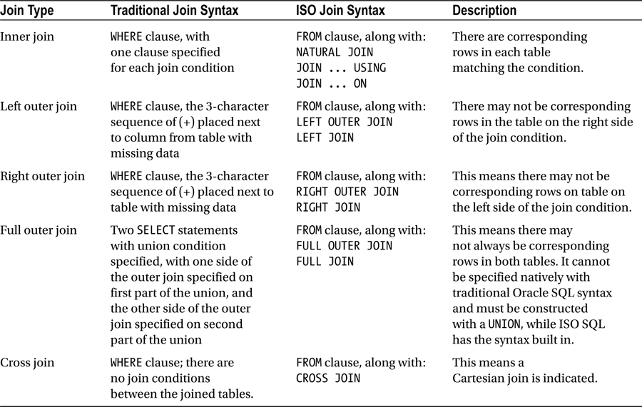
One of the main advantages of the ISO syntax is that fo r multiple table joins, all the join conditions are specified in the FROM clause, and are therefore isolated and easy to see. In Oracle SQL, the join conditions are specified in the WHERE clause, along with any other filtering criteria needed for the query. If you inherited poorly structured SQL code, it is simply harder to read longer and more complex SQL statements that have join conditions and filtering criteria interspersed within a single WHERE clause.

One other type of join not already mentioned is the cross join, which is a Cartesian join, which is all possible combinatinos of all rows from both tables. While this type of join is rarely useful, it can be occasionally beneficial. As a DBA, let’s say you are gathering database size information for your enterprise of databases and are placing the results in a single spreadsheet. You need to get database and host information for each query. You can execute the following query:

  SELECT d.name, i.host_name, round(sum(f.bytes)/1048576) megabytes
  FROM v$database d
  CROSS JOIN v$instance i
  CROSS JOIN v$datafile f
  GROUP BY d.name, i.host_name;
 
NAME      HOST_NAME                       MEGABYTES
--------- ------------------------------ ----------
ORCL      DREGS-PC                             2333

In this case, the v$instance and v$database views contain only a single row, so there is no harm in doing a Cartesian join. The foregoing join could also be written with traditional Oracle SQL:

SELECT d.name, i.host_name, round(sum(f.bytes)/1048576) megabytes
FROM v$database d, v$instance i, v$datafile f
GROUP BY d.name, i.host_name;

Starting with Oracle 12c release 1, if using LEFT OUTER Join syntax, you can now place multiple tables on the left-hand side of the join operation. For instance, see the following query and resulting error message when run in Oracle 11g:

SELECT d.department_name, e.manager_id, l.location_id, sum(e.salary)
FROM departments d, employees e, locations l
WHERE d.department_id = e.department_id
AND e.manager_id = d.manager_id  (+)
AND l.location_id = d.location_id (+)
GROUP BY d.department_name, e.manager_id, l.location_id
ORDER BY 2,3;
 
AND e.manager_id = d.manager_id  (+)
                 *
ERROR at line 4:
ORA-01417: a table may be outer joined to at most one other table

When now running in Oracle 12c, the syntax is now valid and returns an efficient execution plan:

------------------------------------------------------------------
| Id  | Operation                             | Name             |
------------------------------------------------------------------
|   0 | SELECT STATEMENT                      |                  |
|   1 |  SORT GROUP BY                        |                  |
|   2 |   HASH JOIN                           |                  |
|   3 |    TABLE ACCESS BY INDEX ROWID BATCHED| DEPARTMENTS      |
|   4 |     INDEX FULL SCAN                   | DEPT_LOCATION_IX |
|   5 |    TABLE ACCESS FULL                  | EMPLOYEES        |

Problem

You are finding it easiest to think in terms of executing two queries to get your desired results. Your thought process is to execute a first query to get some intermediate results and then executing a second query to get to the results that you really are after.

Solution

It is common that data needs from a relational database are complex enough that the data cannot be retrieved within a simple SQL SELECT statement. Rather than having to run two or more queries serially, it is possible to construct several SQL SELECT statements and place them within a single query. These additional SELECT statements are called subqueries, subselects, or nested selects.

Let’s say you want to get the name of the employee with the highest salary in your company so you can ask your boss for a raise. Since you don’t know what the highest salary is, you first have to run a query to determine the following:

SELECT MAX(salary) FROM employees;
 
MAX(SALARY)
-----------
      24000

Then, knowing what the highest salary is, you could run a second query to get the employee(s) with that salary:

SELECT last_name, first_name
FROM employees
WHERE salary = 24000;
 
LAST_NAME                 FIRST_NAME
------------------------- --------------------
King                      Steven

It’s very simple to combine the foregoing two queries, and construct a single SQL statement with a subquery to accomplish the same task:

SELECT last_name, first_name
FROM employees
WHERE salary =
(SELECT MAX(salary) FROM employees);
 
LAST_NAME                 FIRST_NAME
------------------------- --------------------
King                      Steven

How It Works

Within a SQL statement, a subquery can be placed within the SELECT, WHERE, or HAVING clauses. You can also place a query within the FROM clause, which is also called an inline view, which is addressed in a different recipe. There are several kinds of subqueries that can be constructed:

• Single-row or scalar subquery
• Multiple-row subquery
• Multiple-column subquery
• Correlated subquery (addressed in a different recipe)

In the solution example, the inner query is executed first, and then the results of the inner query are passed to the outer query, which is then executed.

SELECT last_name, first_name
FROM employees
WHERE salary =
(SELECT salary FROM employees WHERE department_id = 30);
 
(SELECT salary FROM employees WHERE department_id = 30)
 *
ERROR at line 4:
ORA-01427: single-row subquery returns more than one row

SELECT last_name, first_name, salary, ROUND((SELECT AVG(salary) FROM employees)) avg_sal
FROM employees
WHERE last_name = 'King';
 
LAST_NAME                 FIRST_NAME               SALARY    AVG_SAL
------------------------- -------------------- ---------- ----------
King                      Steven                    24000       6462

column avg_sal format 99999.99
 
SELECT department_id, ROUND(avg(salary),2) avg_sal
FROM employees
GROUP BY department_id
HAVING avg(salary) > (SELECT AVG(salary) FROM employees)
ORDER BY 2;
 
DEPARTMENT_ID   AVG_SAL
------------- ---------
           40   6500.00
          100   8600.00
           80   8955.88
           20   9500.00
           70  10000.00
          110  10150.00
           90  19333.33
 
8 rows selected.

SELECT department_id, department_name
FROM departments
WHERE department_id = 20
OR department_id = 30
OR department_id = 40;
 
DEPARTMENT_ID DEPARTMENT_NAME
------------- ------------------------------
           20 Marketing
           30 Purchasing
           40 Human Resources

SELECT department_id, department_name
FROM departments
WHERE department_id IN (20,30,40);

SELECT department_id, department_name
FROM departments
WHERE department_id < ANY (20,30,40);
 
SELECT department_id, department_name
FROM departments
WHERE department_id < SOME (20,30,40);
 
DEPARTMENT_ID DEPARTMENT_NAME
------------- ------------------------------
           10 Administration
           20 Marketing
           30 Purchasing

SELECT department_id, department_name
FROM departments
WHERE department_id <= ALL (20,30,40);
 
DEPARTMENT_ID DEPARTMENT_NAME
------------- ------------------------------
           10 Administration
           20 Marketing

SELECT last_name, first_name, department_id, salary
FROM employees
WHERE (department_id, salary) IN
(SELECT department_id, max(salary)
FROM employees
GROUP BY department_id)
ORDER BY department_id;
 
LAST_NAME                 FIRST_NAME           DEPARTMENT_ID     SALARY
------------------------- -------------------- ------------- ----------
Whalen                    Jennifer                        10       4400
Hartstein                 Michael                         20      13000
Raphaely                  Den                             30      11000
Mavris                    Susan                           40       6500
Fripp                     Adam                            50       8200
Hunold                    Alexander                       60       9000
Baer                      Hermann                         70      10000
Russell                   John                            80      14000
King                      Steven                          90      24000
Greenberg                 Nancy                          100      12000
Higgins                   Shelley                        110      12000
 
11 rows selected.

Problem

You are writing a subquery to retrieve data from a given set of tables from your database. In order to retrieve the proper results, you really need to reference the outer query from inside the inner query.

Solution

The correlated subquery is a powerful component of the SQL language. The reason it is called “correlated” is that it allows you to reference the outer query from within the inner query. For example, we want to see the employees in our company whose salary was the minimum for their specific job title:

SELECT department_id, last_name, salary
FROM employees e
WHERE salary =
   (SELECT min_salary
    FROM jobs j
    WHERE e.job_id = j.job_id);
 
DEPARTMENT_ID LAST_NAME           SALARY
------------- --------------- ----------
           50 Olson                 2000
           80 Russell              10000
  

How It Works

Because you reference the outer query from inside the inner query, the process of executing a correlated subquery is essentially the opposite compared to a simple subquery. In a correlated subquery, normally the outer query is executed first, as the inner query needs the data from the outer query in order to be able to process the query and retrieve the results. Depending on the specific query, the optimizer may actually choose to transform the query to a standard join. This can be determined by running an explain plan for a given query. The traditional steps to execute a correlated subquery are as follows. These steps repeat for each row in the outer query:

1. Retrieve row from the outer query.
2. Execute the inner query.
3. The outer query compares the value returned from the inner query.
4. If there is a value match in step 3, the row is returned to the user.

Another type of correlated subquery is to use the EXISTS clause in a subquery. When you use EXISTS, a test is done to see if the inner query returns at least one row. This is the important test that occurs when using the EXISTS operator. As you can see from the following example, the column list of the SELECT clause within the inner query is irrelevant. Something is included there simply to have proper SQL syntax only. If we want to see all the jobs each current employee has ever held in our company, we can use the EXISTS operator to help us get this information:

SELECT employee_id, job_id
FROM job_history h
WHERE EXISTS
(SELECT job_id FROM employees e
WHERE e.job_id = h.job_id)
ORDER BY 1;
 
EMPLOYEE_ID JOB_ID
----------- ----------
        101 AC_ACCOUNT
        101 AC_MGR
        102 IT_PROG
        114 ST_CLERK
        122 ST_CLERK
        176 SA_REP
        176 SA_MAN
        200 AD_ASST
        200 AC_ACCOUNT
        201 MK_REP
 
10 rows selected.

You can also use NOT EXISTSif you want to test the opposite condition within a query. For example, your CEO wants to determine the manager-to-employee ratio within your company. Using the query from the previous example, we can first use the EXISTS operator to determine the number of managers within the company:

SELECT count(*)
FROM employees e
WHERE EXISTS
(SELECT 'TESTING 1,2,3'
FROM employees m
WHERE e.employee_id = manager_id);
 
  COUNT(*)
----------
        18

If we convert EXISTS to NOT EXISTS, we can determine the number of non-managers within the company:

SELECT count(*)
FROM employees e
WHERE NOT EXISTS
(SELECT 'X'
FROM employees m
WHERE e.employee_id = manager_id);
 
 COUNT(*)
---------
       89

Problem

You need to compare data for a subset of columns between two tables. You need to find rows in one table that are missing from the other.

Solution

You can use the Oracle MINUS set operator to compare two sets of data, and show data missing from one of the tables. When using any of the Oracle set operators, the SELECT clauses must be identical in terms of number of columns, and the datatypes of each column.

As an example, you work for a cable television company, and you want to find out what channels are offered free of charge. To test this, you could first simply get a list of the channels offered by your company:

SELECT channel_id FROM channels;
 
CHANNEL_ID
----------
         2
         3
         4
         5
         9

Then, you can run a query to find out which channels have costs associated with them by querying the COSTS table:

SELECT DISTINCT channel_id FROM costs
ORDER BY channel_id;
 
CHANNEL_ID
----------
         2
         3
         4

By quickly doing a visual examination of the results, the free channels are channels 5 and 9. By using a set operator, in this case, MINUS, you can get this result from a single query:

SELECT channel_id
FROM channels
MINUS
SELECT channel_id
FROM costs;
 
CHANNEL_ID
----------
         5
         9

How It Works

It is also very common to use set operators in queries to get more information about the missing data. For instance, you have gotten the free channel list, but you really need to get more information about those free channels, and would like to accomplish everything within a single query:

SELECT channel_id, channel_desc FROM channels
WHERE channel_id IN
(SELECT channel_id
FROM channels
MINUS
SELECT channel_id
FROM costs);
 
CHANNEL_ID CHANNEL_DESC
---------- --------------------
         5 Catalog
         9 Tele Sales

The MINUS operator is very simple to use. However, use MINUS with care. MINUS can easily consume a large amount of temporary tablespace if the data set being retrieved is large, and it can be slow performing as volumes increase. An alternative to using MINUS is to rewrite such a query using an OUTER JOIN. In the first example in the SOLUTION section, see the query repeated below and its associated explain plan:

SELECT channel_id
FROM channels
MINUS
SELECT channel_id
FROM costs;
 
----------------------------------------
| Id  | Operation           | Name     |
----------------------------------------
|   0 | SELECT STATEMENT    |          |
|   1 |  MINUS              |          |
|   2 |   SORT UNIQUE       |          |
|   3 |    TABLE ACCESS FULL| CHANNELS |
|   4 |   SORT UNIQUE       |          |
|   5 |    TABLE ACCESS FULL| COSTS    |
----------------------------------------

Now, see the same query rewritten as an outer join, and it’s associated explain plan:

select h.channel_id
from costs o right join channels h
on o.channel_id = h.channel_id
Where o.channel_id is null and o.cost is null;
 
----------------------------------------
| Id  | Operation           | Name     |
----------------------------------------
|   0 | SELECT STATEMENT    |          |
|   1 |  FILTER             |          |
|   2 |   HASH JOIN OUTER   |          |
|   3 |    TABLE ACCESS FULL| CHANNELS |
|   4 |    TABLE ACCESS FULL| COSTS    |
----------------------------------------

In the foregoing example, using a join method can be more efficient and better performing than using a MINUS set operator. The basic rule of thumb to keep in mind is volume. With very small volumes, MINUS works well. As volumes grow, consider using OUTER JOIN rather than MINUS.

Problem

You need to compare data for a subset of columns between two tables. You need to see all matching rows from those tables.

Solution

You can use the SQL INTERSECT set operator to compare two sets of data and show the matching data between the two tables. Again, when using any of the SQL set operators, the SELECT clauses must be identical in terms of number of columns, and the datatypes of each column.

Using the example of the free channels, we now want to see which channels are not free, and have costs associated with them. By using the INTERSECT set operator, we will see only the matching rows between the two tables:

SELECT channel_id
FROM channels
INTERSECT
SELECT channel_id
FROM costs;
 
CHANNEL_ID
----------
         2
         3
         4

How It Works

When using INTERSECT, think of it as the overlapping data between two tables, based on the column list in the SELECT statement.

Problem

You need to combine the results between two similar SELECT statements, and would like to accomplish it within a single query.

Solution

You can use the SQL set operators UNION or UNION ALL to combine results from two like queries. The difference between using UNION and UNION ALL is that UNION will automatically eliminate any duplicate rows, and each row of the result set will be unique. When using UNION ALL, it will show all matching rows, including duplicate rows. Using UNION ALL may yield better performance than UNION, because a sort to eliminate duplicates is avoided. If your application can eliminate duplicates during processing, it may be worth the performance gained from using UNION ALL.

In Oracle’s sample schemas, we have the SCOTT.EMP table and the HR.EMPLOYEES table. If we want to see all the employees on both tables, we can use a UNION set operator to get the results:

SELECT empno, hiredate FROM scott.emp
UNION
SELECT employee_id, hire_date FROM hr.employees;
 
     EMPNO HIREDATE
---------- ---------
       100 17-JUN-87
       101 21-SEP-89
       102 13-JAN-93
       ...
      7902 03-DEC-81
      7934 23-JAN-82
      7997 15-AUG-11
 
122 rows selected.

How It Works

You are running two queries where you have a nearly identical column list, but let’s say you have one additional column on one table. In this case, we have the COMM column on the SCOTT.EMP table, which is the commission amount an employee has earned. You don’t have an equivalent column on the HR.EMPLOYEES table. By using NULL in the missing column, you can still use a set operator such as UNION as long as you account for any missing columns on either side of the operation:

SELECT empno, mgr, hiredate, sal, deptno, comm
FROM scott.emp
UNION
SELECT employee_id, manager_id, hire_date, salary, department_id, NULL
FROM hr.employees;
 
     EMPNO        MGR HIREDATE         SAL     DEPTNO       COMM
---------- ---------- --------- ---------- ---------- ----------
       100            17-JUN-87      24000         90
       101        100 21-SEP-89      17000         90
       102        100 13-JAN-93      17000         90
       ...
      7369       7902 17-DEC-80        800         20
      7499       7698 20-FEB-81       1600         30        300
      7521       7698 22-FEB-81       1250         30        500
      7566       7839 02-APR-81       2975         20
      7654       7698 28-SEP-81       1250         30       1400

After examining the HR.EMPLOYEES table, there is a column named COMMISSION_PCT. We can derive the actual commission based on this column and add it to the previous query. Also, our manager has told us that he or she wants to see a value in the commission column for all employees, even if they earn no commission:

SELECT empno, mgr, hiredate, sal, deptno, nvl(comm,0)
FROM scott.emp
UNION
SELECT employee_id, manager_id, hire_date, salary, department_id,
nvl(salary*commission_pct/100,0)
FROM hr.employees;
 
     EMPNO        MGR HIREDATE         SAL     DEPTNO NVL(COMM,0)
---------- ---------- --------- ---------- ---------- -----------
       100            17-JUN-87      24000         90           0
       101        100 21-SEP-89      17000         90           0
       102        100 13-JAN-93      17000         90           0
       ...
       147        100 10-MAR-97      12000         80          36
       148        100 15-OCT-99      11000         80          33
       149        100 29-JAN-00      10500         80          21
       ...
      7499       7698 20-FEB-81       1600         30         300
      7521       7698 22-FEB-81       1250         30         500
      7566       7839 02-APR-81       2975         20           0

One point to stress again is that the datatypes for each column also must be the same. For example, we are doing a union between the SCOTT.EMP table and the HR.DEPARTMENTS table and want to see a combined list of the department numbers, along with their locations. However, based on the datatype list, we cannot use an Oracle set operator such as UNION for this, as the location column for each table is different:

SQL> desc scott.dept
 Name                                      Null?    Type
 ----------------------------------------- -------- ------------------------
 
 DEPTNO                                    NOT NULL NUMBER(2)
 DNAME                                              VARCHAR2(14)
 LOC                                                VARCHAR2(13)
 
SQL> desc hr.departments
 Name                                      Null?    Type
 ----------------------------------------- -------- ------------------------
 
 DEPARTMENT_ID                             NOT NULL NUMBER(4)
 DEPARTMENT_NAME                           NOT NULL VARCHAR2(30)
 MANAGER_ID                                         NUMBER(6)
 LOCATION_ID                                        NUMBER(4)
 
SQL> l
  1  SELECT deptno, loc FROM scott.dept
  2  UNION
  3* select department_id, location_id from hr.departments
SQL> /
SELECT deptno, loc FROM scott.dept
               *
ERROR at line 1:
ORA-01790: expression must have same datatype as corresponding expression

Problem

You need to retrieve data from your database based on a range of values for a given column.

Solution

The BETWEEN clause is commonly used to retrieve a range of values from a database. It is most commonly used with dates, timestamps, and numbers but can also be used with alphanumeric data. It is an efficient way of retrieving data from the database when an exact set of values is not known for a column within the WHERE clause. For instance, if we wanted to see all employees that were hired between the year 2000 and through the year 2010, the query could be written as follows:

SELECT last_name, first_name, hire_date
FROM employees
WHERE hire_date BETWEEN to_date('2000-01-01','yyyy-mm-dd')
AND to_date('2010-12-31','yyyy-mm-dd')
ORDER BY hire_date;

When using the BETWEEN clause, it is an efficient way to find a range of values for a column and works for a multitude of datatypes. If you want to get a range of values for a NUMBER datatype as in the SALARY column, a range can be given:

SELECT last_name, first_name, salary
FROM employees
WHERE salary BETWEEN 20000 and 30000
ORDER BY salary;

If you want to add to the foregoing query and get only those employees whose last names are in the first half of the alphabet, you can supply a range to satisfy this request. In order to guarantee all values, we filled out the possible values to the 25-character length of the last_name column:

SELECT last_name, first_name, salary
FROM employees
WHERE salary BETWEEN 20000 and 30000
AND last_name BETWEEN 'Aaaaaaaaaaaaaaaaaaaaaaaaa'
AND 'Mzzzzzzzzzzzzzzzzzzzzzzzz'
ORDER BY salary;

For the above specific example, since the first half of the alphabet is inclusive between “A” and “M”, you could simply the above query by using both BETWEEN in the first clause and a comparison operator in the second clause:

SELECT last_name, first_name, salary
FROM employees
WHERE salary BETWEEN 20000 and 30000
AND last_name < 'N'
ORDER BY salary;

The foregoing two examples demonstrate that the data needed may drive the methods that can and cannot be used when writing a query.

How It Works

One common pitfall when using the BETWEEN clause is with the use of date-based columns, whether it be the DATE datatype, the TIMESTAMP datatype, or any other date-based datatype. If not constructed carefully, desired rows can be missed from the result set.

One way this occurs is that often queries on dates are done using a combination of year, month, and day. It is important to remember that even though the format of the date-based fields on an Oracle database usually defaults to a year, month, and day type of format, the element of time must always be accounted for, else rows can be missed from a query. In this first example, we have an employee, Sarah Bell, who was hired February 4, 1996:

SELECT to_char(hire_date,'yyyy-mm-dd:hh24:mi:ss') hire_date
FROM employees
WHERE email = 'SBELL';
 
HIRE_DATE
-------------------
1996-02-04:12:30:46

If we query the database and don’t consider the time element for any date column, we can omit critical rows from our result set. Therefore it is important to know whether the time portion of the column is included in the makeup of the data. In this case, there is indeed a time element present in the hire_date column:

SELECT last_name, first_name, hire_date
FROM employees
WHERE hire_date = to_date('1996-02-04','yyyy-mm-dd'),
 
no rows selected

When coding SQL, it is important to always assume there is a time element present for any and all date-based columns. Based on that assumption, we can modify the foregoing query to consider the time element in the hire_date column. Two examples are shown. The first uses BETWEEN to delimit the date range, while the second uses comparison operators to delimit the date range. Both return the same result:

SELECT last_name, first_name, to_char(hire_date,'yyyy-mm-dd:hh24:mi:ss') hire_date
FROM employees
WHERE hire_date
BETWEEN TO_DATE('1996-02-04:00:00:00','yyyy-mm-dd:hh24:mi:ss')
AND TO_DATE('1996-02-04:23:59:59','yyyy-mm-dd:hh24:mi:ss'),
 
SELECT last_name, first_name, to_char(hire_date,'yyyy-mm-dd:hh24:mi:ss') hire_date
FROM employees
WHERE hire_date>= TO_DATE('1996-02-04:00:00:00','yyyy-mm-dd:hh24:mi:ss')
    AND hire_date <= TO_DATE('1996-02-04:23:59:59','yyyy-mm-dd:hh24:mi:ss'),

LAST_NAME                 FIRST_NAME           HIRE_DATE
------------------------- -------------------- -------------------
Bell                      Sarah                1996-02-04:12:30:46

Using the foregoing example, we can also use the TRUNC function to eliminate this issue, and although using functions on the left side of the comparison operator generally may hurt performance, the optimizer in this case will still use an index. Below is the explain plan of the query without using TRUNC:

--------------------------------------------------------------
| Id  | Operation                           | Name           |
--------------------------------------------------------------
|   0 | SELECT STATEMENT                    |                |
|   1 |  TABLE ACCESS BY INDEX ROWID BATCHED| EMPLOYEES      |
|   2 |   INDEX RANGE SCAN                  | EMP_HIRE_DT_IX |
--------------------------------------------------------------

In turn, below is the query and resulting plan using the TRUNC function:

SELECT last_name, first_name, hire_date
FROM employees
WHERE trunc(hire_date) = '1996-02-04';
 
LAST_NAME    FIRST_NAME     HIRE_DATE
------------ -------------- ----------
Bell         Sarah          1996-02-04
 
---------------------------------------------------
| Id  | Operation              | Name             |
---------------------------------------------------
|   0 | SELECT STATEMENT       |                  |
|   1 |  VIEW                  | index$_join$_001 |
|   2 |   HASH JOIN            |                  |
|   3 |    INDEX FAST FULL SCAN| EMP_NAME_IX      |
|   4 |    INDEX FAST FULL SCAN| EMP_HIRE_DT_IX   |
---------------------------------------------------

Here is a similar case, where we are performing a SELECT to retrieve all data for a given month specified in the query. In this case, we are retrieving all employees who were hired in the month of September 1997. If we omit the time element from the BETWEEN clause, we can actually omit data that meets the criteria for our query:

    SELECT last_name, first_name, to_char(hire_date,'yyyy-mm-dd:hh24:mi:ss') hire_date
FROM employees
WHERE hire_date
 
BETWEEN TO_DATE('1997-09-01','yyyy-mm-dd')
AND TO_DATE('1997-09-30','yyyy-mm-dd'),
 
LAST_NAME                 FIRST_NAME           HIRE_DATE
------------------------- -------------------- ----------
Chen                      John                 1997-09-28
 
SELECT last_name, first_name,to_char(hire_date,'yyyy-mm-dd:hh24:mi:ss') hire_date
FROM employees
WHERE hire_date
BETWEEN TO_DATE('1997-09-01:00:00:00','yyyy-mm-dd:hh24:mi:ss')
AND TO_DATE('1997-09-30:23:59:59','yyyy-mm-dd:hh24:mi:ss'),
 
 
LAST_NAME    FIRST_NAME     HIRE_DATE
------------ -------------- -------------------
Chen         John           1997-09-28:00:00:00
Sciarra      Ismael         1997-09-30:08:00:00

If you are using a BETWEEN clause or in some way delimit the value range in your query, and there is an index on the column specified in the WHERE clause, the Oracle optimizer can use the index to retrieve the data. By using BETWEEN or some other means to delimit a value range, it is more likely that an index can often be used if one is present. As shown with the following example, you would need to perform an explain plan to validate the use of an index:

SELECT last_name, first_name, salary
FROM employees
WHERE last_name between 'Ba' and 'Bz'
ORDER BY salary;
 
----------------------------------------------------
| Id  | Operation                    | Name        |
----------------------------------------------------
|   0 | SELECT STATEMENT             |             |
|   1 |  SORT ORDER BY               |             |
|   2 |   TABLE ACCESS BY INDEX ROWID| EMPLOYEES   |
|   3 |    INDEX RANGE SCAN          | EMP_NAME_IX |
----------------------------------------------------

Problem

You have null values in some of your database data and need to understand the ramifications of dealing with null values in data. You also need to write queries to correctly deal with such nulls.

Solution

Null values have to be dealt with in a certain manner, depending on whether you are searching for null values in your data in the SELECT clause, or you are attempting to make a determination of what to do when a null value is found in the WHERE clause.

SELECT ename , sal , comm
FROM emp
ORDER BY ename;
 
ENAME             SAL       COMM
---------- ---------- ----------
ADAMS            1100
ALLEN            1600        300
BLAKE            2850
KING             5000
MARTIN           1250       1400

SELECT ename , sal , NVL(comm,0) comm
FROM emp
ORDER BY ename;
 
ENAME             SAL       COMM
---------- ---------- ----------
ADAMS            1100          0
ALLEN            1600        300
BLAKE            2850          0
KING             5000          0
MARTIN           1250       1400

SELECT ename , sal , nvl(comm,0) comm, sal+comm total_comp_no_nvl,
       sal+NVL(comm,0) total_comp_nvl
FROM emp
ORDER BY ename;
 
ENAME             SAL       COMM TOTAL_COMP_NO_NVL TOTAL_COMP_NVL
---------- ---------- ---------- ----------------- --------------
ADAMS            1100          0                             1100
ALLEN            1600        300              1900           1900
BLAKE            2850          0                             2850
KING             5000          0                             5000
MARTIN           1250       1400              2650           2650

SELECT ename , sal ,
NVL2(comm,'Commissioned','Non-Commissioned') comm_status
FROM emp
ORDER BY ename;
 
ENAME             SAL COMM_STATUS
---------- ---------- ----------------
ADAMS            1100 Non-Commissioned
ALLEN            1600 Commissioned
BLAKE            2850 Non-Commissioned
KING             5000 Non-Commissioned
MARTIN           1250 Commissioned

SELECT ename , sal
FROM emp
WHERE comm IS NULL
ORDER BY ename;
 
ENAME             SAL
---------- ----------
ADAMS            1100
BLAKE            2850
KING             5000
 
 
SELECT ename , sal
FROM emp
WHERE comm IS NOT NULL
ORDER BY ename;
 
ENAME             SAL
---------- ----------
ALLEN            1600
MARTIN           1250

SELECT ename , sal
FROM emp
WHERE NVL(comm,0) = 0
ORDER BY ename;
 
ENAME             SAL
---------- ----------
ADAMS            1100
BLAKE            2850
KING             5000

How It Works

It is best to always explicitly handle the possibility of null values, so if a column of a table is nullable, assume nulls exist, else output results can be undesired or unpredictable. One quick check that can be made to determine if a column has null values is to compare a count of rows in the table (COUNT *) to a count of rows for that column (COUNT <column_name>). A count on a nullable column will count only those rows that do not have null values. Here’s an example:

SELECT count(*) FROM emp;
 
  COUNT(*)
----------
        14
 
SELECT count(comm) FROM emp;
 
COUNT(COMM)
-----------
          4

This technique of comparing row count to a count of values in a column is a handy way to check if nulls exist in a column.

Another very useful function that can be used in the handling of null values is the COALESCE function. With COALESCE, you can pass in a series of values, and the function will return the first non-NULL value. If all values within COALESCE are NULL, a NULL value is returned. Here is a simple example:

SELECT coalesce(NULL,'ABC','DEF') FROM dual;
 
COA
---
ABC

Let’s say you wanted to get the shipping address for your customers, and if none were present, you would then get the billing address. If the billing address was not present, you would state that the address is unknown. Using COALESCE, you could achieve this as shown in the following example:

SELECT COALESCE(shipping_address, billing_address,’Address Unknown’)
FROM customers
WHERE cust_id = 9342;
 

All arguments used in a statement with COALESCE must be with the same datatype, else you will receive an error, as shown here:

SELECT coalesce(NULL,123,'DEF') FROM dual;
                         *
ERROR at line 1:
ORA-00932: inconsistent datatypes: expected NUMBER got CHAR

When deciding on whether to use NVL or COALESCE in handling NULL values, evaluate the complexity of the conditions within your statement. NVL is more suited to simple evaluations, while the COALESCE function is better suited to more complex conditions.

Problem

You need to search for a string from a column in the database, but do not know the exact value of the column data.

Solution

When you are unsure of the data values in the columns you are filtering on in your WHERE clause, you can utilize the LIKE operator. Unlike the normal comparison operators such as the equal sign, the BETWEEN clause, or the IN clause, the LIKE operator allows you to search for matches based on a partial string of the column data. When you use the LIKE clause, you need to also use the “%” symbol or the “_” symbol within the data itself in order to search for the data you need. The percent sign is used to replace one to many characters. For example, if you want to see the list of employees that were hired in 1995, regardless of the exact date, the LIKE clause can be used to search for any matches within hire_date that contain the string 1995. When using LIKE with a date or timestamp datatype, you need to ensure that the date format you are using is compatible with your search criteria in your LIKE statement. For instance, if the default date format for your database is DD-MON-YY, then the string 1995 is not compatible with that format and a match would never be found. In order to search in this manner, set your date format within your session before issuing your query:

alter session set nls_date_format = 'yyyy-mm-dd';
 
Session altered.
 
SELECT employee_id, last_name, first_name, hire_date
FROM employees
WHERE hire_date LIKE '%1995%';
 
EMPLOYEE_ID LAST_NAME                 FIRST_NAME           HIRE_DATE
----------- ------------------------- -------------------- ----------
        122 Kaufling                  Payam                1995-05-01
        115 Khoo                      Alexander            1995-05-18
        137 Ladwig                    Renske               1995-07-14
        141 Rajs                      Trenna               1995-10-17

An easy way to remedy having to worry about the date format of your session is to simply use the TO_CHAR function within the query. The advantage of this method is it is very easy to code, without having to worry about your session’s date format. See the following equivalent example:

SELECT employee_id, last_name, first_name, hire_date
FROM employees
WHERE to_char(hire_date,'yyyy') = '1995';

Yet a third way to do the same thing is to use the EXTRACT function:

SELECT employee_id, last_name, first_name, hire_date
FROM employees
WHERE extract(year from hire_date) = '1995';

The underscore symbol (“_”) is used to replace exactly one character. Let’s say you were looking for an employee that had a last name of “Olsen” or “Olson,” but were unsure of the spelling. In a single query, you can use the underscore in conjunction with the LIKE clause to find all employees with that name variation in your database:

SELECT last_name, first_name, phone_number
FROM employees
WHERE last_name like 'Ols_n';
 
LAST_NAME                 FIRST_NAME           PHONE_NUMBER
------------------------- -------------------- --------------------
Olsen                     Christopher          011.44.1344.498718
Olson                     TJ                   650.124.8234

How It Works

The LIKE clause is extremely useful for finding data within your database when you are unsure of the exact column values stored within the data. There are performance ramifications that need to be considered when using the LIKE clause. The primary consideration is that when the LIKE clause is used, the likelihood of the optimizer using an index to aid in retrieving the data are reduced, especially if the wild card character is placed on the leading edge of the value. Since an index is based on a complete value for a column, having to search for only a portion of the complete value of a column is problematic for the optimizer to be able to use an index.

Using our foregoing example of finding employees that started during the year 1995, here is the explain plan for that query:

-------------------------------------------------------------------------------
| Id  | Operation         | Name      | Rows  | Bytes | Cost (%CPU)| Time     |
-------------------------------------------------------------------------------
|   0 | SELECT STATEMENT  |           |     5 |   135 |     3   (0)| 00:00:01 |
|*  1 |  TABLE ACCESS FULL| EMPLOYEES |     5 |   135 |     3   (0)| 00:00:01 |
-------------------------------------------------------------------------------
 
Predicate Information (identified by operation id):
---------------------------------------------------
 
   1 - filter(INTERNAL_FUNCTION("HIRE_DATE") LIKE '%1995%')

If you need to use the LIKE clause for a given query, do not expect an index to be used. There can be exceptions, however. A couple of scenarios include if you have an ORDER BY clause on an indexed column. If we take the previous example and add an ORDER BY clause, the optimizer will use the index to assist in sorting the data:

SELECT employee_id, last_name, first_name, hire_date
FROM employees
WHERE hire_date LIKE '%1995%'
ORDER BY hire_date;
 
------------------------------------------------------
| Id  | Operation                   | Name           |
------------------------------------------------------
|   0 | SELECT STATEMENT            |                |
|   1 |  TABLE ACCESS BY INDEX ROWID| EMPLOYEES      |
|   2 |   INDEX FULL SCAN           | EMP_HIRE_DT_IX |
------------------------------------------------------

The INDEX FULL SCAN shown in the foregoing example isn’t the most efficient index usage but is still more efficient than a full table scan. If your query only queried on column(s) that are part of an index, the optimizer may choose to use the index, even with the LIKE clause:

SELECT employee_id, hire_date
FROM employees
WHERE hire_date LIKE '%1995%';
 
---------------------------------------------------
| Id  | Operation              | Name             |
---------------------------------------------------
|   0 | SELECT STATEMENT       |                  |
|   1 |  VIEW                  | index$_join$_001 |
|   2 |   HASH JOIN            |                  |
|   3 |    INDEX FAST FULL SCAN| EMP_EMP_ID_PK    |
|   4 |    INDEX FAST FULL SCAN| EMP_HIRE_DT_IX   |
---------------------------------------------------

Each statement is different, along with the environment, statistics, and other factors relating to your specific database. The best course of action is to always run an explain plan, as one given statement may produce different execution plans on different databases, depending on the circumstances.

Sometimes it is very possible for an underscore to be part of the data that is being searched. In these cases, it is important to preface the underscore with the escape character. If you are a DBA and are searching for a tablespace name in your database, which easily can contain the underscore character, make sure you consider that underscore is a wildcard symbol and must be considered. See the following example:

SELECT tablespace_name FROM dba_tablespaces
WHERE tablespace_name like '%EE_DATA';
 
TABLESPACE_NAME
------------------------------
EMPLOYEE_DATA
EMPLOYEE1DATA

If you insert an escape character within the query, you can avoid getting undesired results. By inserting the escape character directly in front of the underscore, then the underscore will be considered as part of the data, rather than a substitution character:

SELECT tablespace_name FROM dba_tablespaces
WHERE tablespace_name LIKE '%EE^_DATA' ESCAPE '^';
 
TABLESPACE_NAME
------------------------------
EMPLOYEE_DATA

The benefit of the LIKE clause is the flexibility it gives you in finding data based on a partial value of the column data. The likely trade-off is performance. Queries using the LIKE clause are often much less likely to use an index. As an alternative to LIKE, the BETWEEN clause, although not as simple to code within your SQL statement, can generally be more likely to use an index.

In the TO_CHAR example of the “Solution” section, you will note that the TO_CHAR function is placed on the left side of the comparison operator. Generally, when this occurs, it means no index on the filtering column will be used (see Recipe 8-14 for more discussion on this topic). However, with certain Oracle functions and the manner in which they are translated, an index still may be used. The only way to be certain is to simply run an explain plan on your query. For our foregoing query using TO_CHAR, it still used an index even though the function was placed on the left side of the comparison operator:

SELECT employee_id, last_name, first_name, hire_date
FROM employees
WHERE to_char(hire_date,'yyyy') = '1995'
ORDER BY hire_date;
----------------------------------------------------
| Id  | Operation                   | Name         |
----------------------------------------------------
|   0 | SELECT STATEMENT            |              |
|   1 |  TABLE ACCESS BY INDEX ROWID| EMPLOYEES    |
|   2 |   INDEX FULL SCAN           | EMPLOYEES_I1 |
----------------------------------------------------

Problem

You are getting an excessive amount of hard parsing for your SQL statements and want to lower the number of SQL statements that go through the hard-parse process.

Solution

Implementing bind variables within an application can tremendously improve the efficiency and performance of queries. Bind variables are used to replace literals within a query. By placing bind variables within your SQL statements, the statements can be re-used in memory and do not have to go through the entire expensive SQL parsing process.

Here is an example of a normal SQL statement, with literal values shown in the WHERE clause:

SELECT employee_id, last_name || ', ' || first_name employee_name
FROM employees
WHERE employee_id = 115;
 
EMPLOYEE_ID EMPLOYEE_NAME
----------- -------------------------
        115 Khoo, Alexander

There are a couple of ways to define bind variables within Oracle. First, you can simply use SQL Plus. To accomplish this within SQL Plus, you first need to define a variable, along with a datatype to the variable. Then, you can use the exec command, which actually will run a PL/SQL command to populate the variable with the desired value. Notice that when referencing a bind variable in SQL Plus, it is prefaced with a colon:

SQL> variable g_emp_id number
SQL> exec :g_emp_id := 115;
 
PL/SQL procedure successfully completed.

After you have defined a variable and assigned a value to it, you can simply substitute the variable name within your SQL statement. Again, since it is a bind variable, you need to preface it with a colon:

SELECT employee_id, last_name || ', ' || first_name employee_name
FROM employees
WHERE employee_id = :g_emp_id;
 
EMPLOYEE_ID EMPLOYEE_NAME
----------- -------------------------
        115 Khoo, Alexander

You can also assign variables within PL/SQL. The nice advantage of PL/SQL is that just by using variables in PL/SQL, they are automatically bind variables. And, unlike in SQL*Plus, no colon is required when referencing a variable that was defined within the PL/SQL block:

SQL> set serveroutput on
  1  DECLARE
  2    v_emp_id employees.employee_id%TYPE := 200;
  3    v_last_name employees.last_name%TYPE;
  4    v_first_name employees.first_name%TYPE;
  5  BEGIN
  6    SELECT last_name, first_name
  7    INTO v_last_name, v_first_name
  8    FROM employees
  9    WHERE employee_id = v_emp_id;
 10  dbms_output.put_line('Employee Name = ' || v_last_name || ', ' || v_first_name);
 11* END;
SQL> /
Employee Name = Whalen, Jennifer

How It Works

When bind variables are used, it increases the likelihood that a SQL statement can be re-used within the shared pool. Oracle uses a hashing algorithm to assign a value to every unique SQL statement. If literals are used within a SQL statement, the hash values between two otherwise identical statements will be different. By using the bind variables, the statements will have the same hash value within the shared pool, and part of the expensive parsing process can be avoided.

alter session set sql_trace=true;

SELECT dbms_debug_jdwp.current_session_id sid,
dbms_debug_jdwp.current_session_serial serial#
from dual;
 
       SID    SERIAL#
---------- ----------
        64      21713
 
exec dbms_monitor.session_trace_enable(session_id=>64,serial_num=>21713);

BEGIN
FOR i IN 100..206
LOOP
UPDATE employees
SET salary=salary*1.03
WHERE employee_id = i;
END LOOP;
COMMIT;
END;

UPDATE EMPLOYEES_BIG SET SALARY=SALARY*1.03
WHERE
 EMPLOYEE_ID = :B1
 
 
call     count       cpu    elapsed    disk   query    current        rows
------- ------  -------- ---------- ------- ------- ----------  ---------
Parse        1      0.00       0.00       0       0          0           0
Execute     16    142.10     380.62       0     729   13979390    12583424
Fetch        0      0.00       0.00       0       0          0           0
------- ------  -------- ---------- ------- ------- ----------  ---------
total       17    142.11     380.62       0     729   13979390    12583424
 

BEGIN
FOR i IN 100..206
LOOP
execute immediate 'UPDATE employees SET salary=salary*1.03 WHERE employee_id = ' || i;
END LOOP;
COMMIT;
END;

SQL ID: 5ad0n7d74j9au Plan Hash: 751015319
UPDATE employees SET salary=salary*1.03
WHERE
 employee_id = 206
 
 
call     count       cpu    elapsed   disk   query    current        rows
------- ------  -------- ---------- ------ ------- ----------  ----------
Parse        1      0.00       0.01      0       0          0           0
Execute      1      0.04      21.12      0      27        265         256
Fetch        0      0.00       0.00      0       0          0           0
------- ------  -------- ---------- ------ ------- ----------  ----------
total        2      0.04      21.13      0      27        265         256

OVERALL TOTALS FOR ALL RECURSIVE STATEMENTS
 
call     count       cpu    elapsed   disk   query    current        rows
------- ------  -------- ---------- ------ ------- ----------  ----------
Parse      168      0.07       0.08      0       0        120           0
Execute    168    261.00     707.14      4     911   27688705    12583424
Fetch      151      0.00       0.01      2     405          0         103
------- ------  -------- ---------- ------ ------- ----------  ----------
total      487    261.08     707.24      6    1316   27688825    12583527
 
 
       1  session in tracefile.
     109  user  SQL statements in trace file.
       0  internal SQL statements in trace file.
     109  SQL statements in trace file.
     109  unique SQL statements in trace file.
    1016  lines in trace file.
       8  elapsed seconds in trace file.

BEGIN
FOR i IN 100..206
LOOP
execute immediate 'UPDATE employees SET salary=salary*1.03 WHERE employee_id = :empno' USING i;
END LOOP;
COMMIT;
END;
 
SQL ID : 4y09bqzjngvq4
update employees set salary=salary*1.03
where
 employee_id = :empno
 
call     count       cpu    elapsed    disk  query    current        rows
------- ------  -------- ---------- ------- ------ ----------  ----------
Parse        1      0.00       0.00       0      0          0           0
Execute     16    146.65     399.63       3    730   13983401    12583424
Fetch        0      0.00       0.00       0      0          0           0
------- ------  -------- ---------- ------- ------ ----------  ----------
total       17    146.65     399.63       3    730   13983401    12583424

Problem

You have queries that should be using indexes, but instead are doing full table scans. You want to avoid performing full table scans when the optimizer could be using an index to retrieve the data.

Solution

When constructing a SQL statement, a fundamental rule to try to always observe in the WHERE clause, if possible, is to avoid doing function calls on indexed columns, which typically are on the left side of the comparison operator. In these cases, the optimizer will not use any available index, unless a function-based index exists that the query can use. A function essentially turns a column into a literal value, and therefore the Oracle optimizer does not recognize that converted value as a column any longer but as a value instead.

Here, we’re trying to get a list of all the employees that started since the year 1999. Because we placed a function on the left side of the comparison operator, the optimizer will choose a full table scan, even though the HIRE_DATE column is indexed:

SELECT employee_id, salary, hire_date
FROM employees
WHERE TO_CHAR(hire_date,'yyyy-mm-dd') >= '2000-01-01';
 
---------------------------------------
| Id  | Operation         | Name      |
---------------------------------------
|   0 | SELECT STATEMENT  |           |
|   1 |  TABLE ACCESS FULL| EMPLOYEES |
---------------------------------------

By moving the function to the right side of the comparison operator and leaving HIRE_DATE as a pristine column in the WHERE clause, the optimizer can now use the index on HIRE_DATE:

SELECT employee_id, salary, hire_date
FROM employees
WHERE hire_date >= TO_DATE('2000-01-01','yyyy-mm-dd'),
 
-------------------------------------------------
| Id  | Operation                   | Name      |
-------------------------------------------------
|   0 | SELECT STATEMENT            |           |
|   1 |  TABLE ACCESS BY INDEX ROWID| EMPLOYEES |
|   2 |   INDEX RANGE SCAN          | EMP_I5    |
-------------------------------------------------

How It Works

Functions are wonderful tools to convert a value or return the desired value based on what you need from the database, but they can be a performance killer if used incorrectly within a SQL statement. Make sure all functions apply to constants, to unindexed columns, or at least to the least-selective indexed column when two indexed columns are involved in a comparison. Then the optimizer will be able to use any indexes on columns specified in the WHERE clause. This rule holds true for most functions. In certain cases, it is possible Oracle will still use an index even if a function is on the left side of the comparison operator, but this is usually the exception. See Recipe 8-12 for an example of this.

Keep in mind that the datatype for a given column in the WHERE clause may change how the SQL statement needs to be modified to move the function to the right side of the comparison operator. With the following example, we had to change the comparison operator in order to effectively move the function:

SELECT last_name, first_name
FROM employees
WHERE SUBSTR(phone_number,1,3) = '515';
 
---------------------------------------
| Id  | Operation         | Name      |
---------------------------------------
|   0 | SELECT STATEMENT  |           |
|   1 |  TABLE ACCESS FULL| EMPLOYEES |
---------------------------------------

In order to effectively get all numbers in the 515 area code, we can use a BETWEEN clause and capture all possible values. We can also use a LIKE clause, as long as the wildcard character is on the trailing end of the condition. By using either of these methods, the optimizer changed the execution plan to use an index:

SELECT last_name, first_name
FROM employees
WHERE phone_number BETWEEN '515.000.0000' and '515.999.9999';
 
SELECT last_name, first_name
FROM employees
WHERE phone_number LIKE'515%';
 
---------------------------------------------------
| Id  | Operation              | Name             |
---------------------------------------------------
|   0 | SELECT STATEMENT       |                  |
|   1 |  VIEW                  | index$_join$_001 |
|   2 |   HASH JOIN            |                  |
|   3 |    INDEX RANGE SCAN    | EMP_PH_NO        |
|   4 |    INDEX FAST FULL SCAN| EMP_NAME_IX      |
---------------------------------------------------

Problem

You need a table or a view of data that does not exist to construct a needed query and do not have the authority to create such a table or view on your database.

Solution

At times, within a single SQL statement, you want to create a table “on the fly” that is used solely for your query and will never be used again. In the FROM clause of your query, you normally place the name of your table or view on which to retrieve the data. In cases where a needed view of the data does not exist, you can create a temporary view of that data with what is called an “inline view,” where you specify the characteristics of that view right in the FROM clause of your query:

SELECT last_name, first_name, department_name dept, salary
FROM employees e join
       ( SELECT department_id, max(salary) high_sal
         FROM employees
         GROUP BY department_id ) m
USING (department_id) join departments
USING (department_id)
WHERE e.salary = m.high_sal
ORDER BY SALARY desc;
 
LAST_NAME                 FIRST_NAME           DEPT                     SALARY
------------------------- -------------------- -------------------- ----------
King                      Steven               Executive                 24000
Russell                   John                 Sales                     14000
Hartstein                 Michael              Marketing                 13000
Greenberg                 Nancy                Finance                   12000
Higgins                   Shelley              Accounting                12000
Raphaely                  Den                  Purchasing                11000
Baer                      Hermann              Public Relations          10000
Hunold                    Alexander            IT                         9000
Fripp                     Adam                 Shipping                   8200
Mavris                    Susan                Human Resources            6500
Whalen                    Jennifer             Administration             4400

In the foregoing query, we are getting the employees with the highest salary for each department. There isn’t such a view in our database. Moreover, there isn’t a way to directly join the employees table to the departments table to retrieve this data within a single query. Therefore, the inline view is created as part of the SQL statement and holds only the key information we needed—it has the high salary and department information, which now can easily be joined to the employees table based on the employee with that matching salary.

How It Works

Inline views, as with many components of the SQL language, need to be used carefully. While extremely useful, if misused or overused, inline views can cause database performance issues, especially in terms of the use of the temporary tablespace. Since inline views are created and used only for the duration of a query, their results are held in the program global memory area and, if too large, the temporary tablespace. Before using an inline view, the following questions should be considered:

1. Most importantly, how often will the SQL containing the inline view be run?  If only once or rarely, then it might be best to simply execute the query and not worry about any potential performance impact.
2. How many rows will be contained in the inline view?
3. What will the row length be for the inline view?
4. How much memory is allocated for the pga_aggregate_target or memory_target setting?
5. How big is the temporary tablespace that is used by your Oracle user or schema?

If you have a simple ad hoc query you are doing, this kind of analysis may not be necessary. If you are creating a SQL statement that will run in a production environment, it is important to perform this analysis, as if all the temporary tablespace is consumed by an inline view, it affects not only the completion of that query, but also the successful completion of any processing for any user that may use that specific temporary tablespace. In many database environments, there is only a single temporary tablespace. Therefore, if one user process consumes all the temporary space with a single operation, this affects the operations for every user in the database.

Consider the following query:

WITH service_info AS
(SELECT
product_id,
geographic_id,
sum(qty) quantity
FROM services
GROUP BY
product_id,
geographic_id),
product_info AS
(SELECT product_id, product_group, product_desc
FROM products
WHERE source_sys = 'BILLING'),
billing_info AS
(SELECT journal_date, billing_date, product_id
FROM BILLING
WHERE journal_date = TO_DATE('2013-08-15', 'YYYY-MM-DD'))
SELECT
product_group,
product_desc,
journal_date,
billing_date,
sum(service_info.quantity)
FROM service_info JOIN product_info
ON service_info.product_id = product_info.product_id JOIN billing_info
ON  service_info.product_id = billing_info.product_id
WHERE
service_info.quantity > 0
GROUP BY
product_group,
product_desc,
journal_date,
billing_date;

The WITH clause is also known as subquery factoring. In the foregoing query, there are three portions created either as inline views or temporary tables: the SERVICE_INFO view, the PRODUCT_INFO view, and the BILLING_INFO view. Each of these queries will be processed and the results stored in the program global area or the temporary tablespace before finally processing the true end-user query, which starts with the final SELECT statement shown in the query. While efficient in that the desired results can be done by executing a single query, the foregoing query, depending on the size of the data within the tables, can be tremendously inefficient to process, as storing potentially millions of rows in the temporary tablespace uses critical resources needed by an entire community of users that use the database. In examples such as these, it is generally more efficient at the database level to create permanent objects such as tables or materialized views that hold the data. Then, the final query can be extracted from joining the three permanent tables to generate the results. While this may be more upfront work by the development team and the DBA, it could very well pay dividends if the query is run on a regular basis. Furthermore, as complexity increases with a SQL statement, ease of maintenance decreases. So, overall, it is more efficient, and usually more maintainable, to break a complex statement into chunks.

Inline views provide great benefit. However, do the proper analysis and investigation prior to implementing the use of such a view in a production environment.

Problem

You have queries that use the NOT clause that are not performing adequately and wish to modify them to improve performance.

Solution

Just as often as we query our database for equality conditions, we will query our database for non-equality conditions. It is the nature of retrieving data from a database and the nature of the SQL language to allow users to do this.

There are performance drawbacks in using the NOT clause within your SQL statements, as they trigger full table scans. Here’s an example query from a previous recipe:

SELECT last_name, first_name, salary, email
FROM employees_big
WHERE department_id NOT IN(20,30)
AND commission_pct > 0;
 
Elapsed:00:00:21.65
 
----------------------------------------------------------------------
|Id |Operation         |Name         |Rows|Bytes|Cost (%CPU)|Time    |
----------------------------------------------------------------------
|  0|SELECT STATEMENT  |             |   1|   43|  535   (1)|00:00:01|
|* 1| TABLE ACCESS FULL|EMPLOYEES_BIG|   1|   43|  535   (1)|00:00:01|
----------------------------------------------------------------------

Even though we have an index on the department_id column, by using the NOT clause we cause Oracle to bypass the use of that index in order to properly search and ensure all rows were not those in department 20 or 30. One of the easiest ways to avoid the NOT IN clause in this example is simply to convert it to an IN clause. While it may be simpler to code the NOT IN because there are less values, using IN will more likely use an index. In the following example, the NOT IN has been converted to an IN clause showing all values except the ones shown in the NOT IN clause:

SELECT last_name, first_name, salary, email
FROM employees_big
WHERE department_id IN(10,40,50,60,70,80,90,100,110)
and commission_pct > 0;
 
Elapsed:00:00:00.02
 
------------------------------------------------------------------------------
|Id|Operation                  |Name          |Rows|Bytes|Cost (%CPU)|Time    |
-------------------------------------------------------------------------------
| 0|SELECT STATEMENT           |              |   1|   43|   11   (0)|00:00:01|
| 1| INLIST ITERATOR           |              |    |     |           |        |
|*2|  TABLE ACCESS BY          |EMPLOYEES_BIG |   1|   43|   11   (0)|00:00:01|
            INDEX ROWID BATCHED
|*3|   INDEX RANGE SCAN        |EMP_BIG_DEPTNO|   5|     |   10   (0)|00:00:01|
-------------------------------------------------------------------------------

Note now that after our change, the query now uses an index and is substantially faster in run time. Keep in mind that based on the make-up of the data in the table, the optimizer may still decide it is more optimal to do a full table scan, even if there is an index on the filtering column. In these cases, one option to improve performance is to use parallelism (discussed in Chapter 15).

Another way to get the optimizer to use an index is to use the NOT EXISTS clause. Using the foregoing example and modifying it to use a NOT EXISTS clause, an index is used:

SELECT last_name, first_name, salary, email
FROM employees
WHERE NOT EXISTS
(SELECT department_id FROM departments
WHERE department_id in(20,30))
AND commission_pct > 0;
 
-----------------------------------------------------------------------
|Id|Operation           |Name         |Rows|Bytes|Cost (%CPU)|Time    |
------------------------------------------------------------------------
| 0|SELECT STATEMENT    |             |   1|   40|  536   (1)|00:00:01|
|*1| FILTER             |             |    |     |           |        |
|*2|  TABLE ACCESS FULL |EMPLOYEES_BIG|   1|   40|  535   (1)|00:00:01|
| 3|  INLIST ITERATOR   |             |    |     |           |        |
|*4|   INDEX UNIQUE SCAN|DEPT_ID_PK   |   2|    8|    1   (0)|00:00:01|
-----------------------------------------------------------------------

How It Works

You can effectively use the NOT clause several ways:

• Comparison operators ('<>', '!=', '^=')
• NOT IN
• NOT LIKE

By using NOT, each of the following queries has the same basic effect in that it will negate the use of any possible index on the columns to which NOT applies:

SELECT last_name, first_name, salary, email
FROM employees
WHERE department_id != 20
AND commission_pct > 0;
 
SELECT last_name, first_name, salary, email
FROM employees
WHERE department_id NOT IN(20,30)
AND commission_pct > 0;
 
SELECT last_name, first_name, salary, email
FROM employees
WHERE hire_date NOT LIKE '2%'
AND commission_pct > 0;
 
---------------------------------------
| Id  | Operation         | Name      |
---------------------------------------
|   0 | SELECT STATEMENT  |           |
|   1 |  TABLE ACCESS FULL| EMPLOYEES |
---------------------------------------

At times, a full table scan is simply required. Even if an index is present, if you need to read more than a certain percentage of rows of a table, the Oracle optimizer may perform a full table scan regardless of whether an index is present. Still, if you simply try to avoid using NOT where possible, you may be able to improve performance of your queries.

Problem

You are performing a series of DML activities and want to better manage the units of work and the recoverability of your transactions.

Solution

With the use of savepoints, you can split up transactions more easily into logical chunks and can manage them more effectively upon failure. With the use of savepoints, you can roll back a series of DML statements to an incremental savepoint you have created. Within your SQL session, simply create a savepoint at an appropriate place during your processing that allows you to more easily isolate a “logical unit of work.” With larger units of work, savepoints can help overall database performance by reducing the amount of data held in undo tablespaces at any given point in time. The following is an example showing how to create a savepoint:

SQL> savepoint A;
 
Savepoint created.

If you have an online bookstore, for instance, and you have a customer placing an online order, when he or she submits an order, a logical unit of work for this transaction would be as follows:

• Adding a row to the orders table
• Adding one to many rows to the orderitems table

When processing this online order, you will want to commit all the information for the order and all items for an order as one transaction. This particular customer order represents multiple database DML statements but needs to be processed one at a time to preserve the integrity of the order; therefore, it can be regarded as one “logical unit of work.” By using savepoints, you can more easily process multiple DML statements as logical units of work. When a savepoint is created, it is essentially creating an alias based on a system change number (SCN). After creating a savepoint, you then have the luxury to roll back a transaction to that SCN based on the savepoint you created.

How It Works

Let’s say your company has established two new departments, as well as employees for those departments. You need to insert rows in the corresponding DEPT and EMP tables, but you need to do this in one logical, grouped transaction. In case of an error, you can roll back to the point the last logical transaction completed. First, we can see a current picture of the DEPT table:

SELECT * FROM dept;
 
    DEPTNO DNAME          LOC
---------- -------------- -------------
        10 ACCOUNTING     NEW YORK
        20 RESEARCH       DALLAS
        30 SALES          CHICAGO
        40 OPERATIONS     BOSTON

We first insert the information for the first department into the DEPT and EMP tables, and then create a savepoint:

INSERT INTO dept VALUES (50,'PAYROLL','LOS ANGELES'),
 
1 row created.
 
INSERT INTO emp VALUES (7997,'EVANS','ACCTNT',7566,'2011-08-15',900,0,50);
 
1 row created.
 
savepoint A;
 
Savepoint created.

We then start processing information for the second department. Let’s say in the middle of the transaction, an unknown error occurs between the insert into the DEPT table and the insert into the EMP table. In this case, we know this transaction of inserting the information into the recruiting department must be rolled back. At the same time, we wish to commit the transaction to the payroll department. Using the savepoint we created, we can commit a portion of the transaction, while rolling back the portion of the transaction we do not want to keep:

INSERT INTO dept VALUES (60,'RECRUITING','DENVER'),
 
1 row created.
 
ROLLBACK to savepoint A;
 
Rollback complete.
 
COMMIT;
 
Commit complete.

Because of the savepoint, our rollback rolled back the incomplete transaction only for department 60, and the subsequent commit wrote the complete transaction for department 50 to the database in both the DEPT and EMP tables:

SELECT * FROM dept;
 
    DEPTNO DNAME          LOC
---------- -------------- -------------
        10 ACCOUNTING     NEW YORK
        20 RESEARCH       DALLAS
        30 SALES          CHICAGO
        40 OPERATIONS     BOSTON
        50 PAYROLL        LOS ANGELES
 
SELECT * FROM emp
WHERE empno = 7997;
 
     EMPNO ENAME      JOB              MGR HIREDATE    SAL       COMM  DEPTNO
---------- ---------- --------- ---------- ---------- ---- ---------- -------
      7997 EVANS      ACCTNT          7566 2011-08-15  900          0      50

There are many similar mechanisms or coding techniques you can use in programming languages such as PL/SQL. The SAVEPOINT command in the SQL language is a simple way to manage transactions without having to code more complex programming structures.