Azure SQL is not a traditional relational database platform. Every modern database must enable you to use various data formats for different scenarios. Although traditional normalized relational format is battle-tested and proven as optimal technology for a wide range of different scenarios, in some cases, you might find that some other formats might be the better fit for the problem that you are solving.
One common example is denormalization. Traditionally, you are representing domain objects as a set of tables in the so-called normal form described in the previous chapters. This is a well-known database design technique where every complex domain structure, such as list or array, is placed in a separate table. The normalized model is optimal for highly concurrent workloads where many threads simultaneously update and read different parts of the domain object without affecting the threads that are updating other parts. However, if you have a workload where one thread accesses a single object at a time, a highly normalized database might force you to join a lot of tables to reconstruct the domain object from its physical parts. In this case, you might consider serializing the object as a single unit instead of decomposing it.
Azure SQL enables you to use both relational and non-relational structures in the same physical data model.
The ability to work with relational, structured, or several types of semi-structured formats categorizes Azure SQL as a Multi-Model database. If you visit https://db-engines.com/en/ranking site that scores popularity of databases, you might notice that all highly ranked relational databases are also classified as multi-model databases, because supporting various data formats is a must-have requirement for all modern database systems.
Leveraging multi-model capabilities in database design
Before we deep dive into multi-model capabilities of Azure SQL, let us see when you should use them in your applications. Some software engineers like NoSQL concepts because they make a database easier to use and don’t require (apparently) a lot of design upfront, and as such, you can start to use it right away without putting too much effort, and it also doesn't require complex joins between tables. Others prefer relational model because it is battle-tested and guarantees that you may model any domain regardless of complexity. As a mature software engineer, you should not use dogmatic architectural decisions based on some arbitrary preference. The choice between relational and non-relational models or their combination should be based on the domain model of your application.
If you are using something like Domain-Driven Development (DDD) , you are probably identifying Aggregates in your domain. Aggregate objects in DDD are the core entities in your domain model that represent the main access point for data and reference other entities and values. As an example, Customer might be the primary entity that you will use in your sales management module. This entity has some value objects and the reference to the other entities like Order or Invoice. If you know that client code will access customer orders and invoices through Customer object, then Customer is an aggregate that binds other entities that belong to him and represents the main access point for any external component that references any of the entities.
Do not confuse Aggregates in DDD with aggregate functions (SUM, AVG, MAX) in SQL terminology.
The dogmatic NoSQL approach would be to serialize the entire Customer aggregate and all related entities (Orders, Invoices) as one big collection that contains everything that you need in your application layer. This is a perfect choice for the applications that can fetch all necessary data using a single data access operation. Dogmatic relational approach would be to break every entity into a separate highly normalized table so different services in your application can access only a minimal set of information that they need. This is a perfect choice for highly concurrent applications where different threads at the same time access and modify different parts of entities or aggregates.
If you have big and complex forms where you need to preload both Order and Invoice entities after fetching Customer root aggregate and update information in Customer, Invoice, and Order entities once you save data on the form, it makes sense to store dependent entities as denormalized collections. This way you will read and persist all data with a single data access and avoid complex joins that gather data and transactions that span over multiple tables.
If you know that different forms and services in your application might simultaneously update Invoice or Order entities that belong to the same Customer aggregate or you are frequently using lazy loading techniques, it makes sense to break entities into separate tables. This way, you can implement granular services that write and read only the objects that are needed. Breaking the entities to separate tables increases concurrency of your system, because different transactions can touch different parts of the entities without blocking each other. Otherwise, they would be synchronized and potentially blocked on each other.
The application access patterns are the key factors that can guide your decision to use normalized or denormalized models.
Classifying domain models
Highly normalized relational model where you have dependencies and relationships between the entities (like classes in UML diagrams). This model is a perfect choice for highly concurrent applications and services updating or loading different parts of entities.
Graph models are special kinds of models where nodes are interconnected with edges forming logical graph structure. This structure is a perfect choice for services that frequently break or establish bounds between the entities and traverse through the relations finding best paths or “friend-of-a-friend” type of analytics.
Non-relational data where information is self-contained into the isolated data entities with very weak or non-existing relationships between them. This structure is perfect for the services that read and save domain objects as a single unit.
Structured where all data entities have uniform or fixed schema. These types of entities can be easily visualized as rows and columns in Excel tables or serialized in CSV format.
Semi-structured where data entities have some structure, but it is not always strict or uniform. Data entities have some common properties that are repeated across all entities, and some properties vary. Imagine a key-value collection with the different keys across entities or a hierarchically organized document with some missing values and sub-objects. These objects are typically serialized in JSON format.
Unstructured data where patterns highly vary between data entities, and it is hard to find the common structure. The typical examples can be textual documents, images, or videos – there is a well-defined format that enables you to read information, but a combination of information in images makes them very different.
Azure SQL is the best fit for relational structured and also a good fit for relational semi-structured data. The querying capabilities of SQL language enable you to apply the same processing rules over a large set of structured and semi-structured data and also easily traverse through foreign key and edge relationships.
Structured information without relationships might be more efficiently stored as CSV or Excel files, especially if you need to store a large amount of data on Azure Data Lake or Azure Blob Storage. It doesn’t mean that you are losing query capabilities because Azure SQL still enables you to easily load these files from external storage and query them as in-database rows. Semi-structured and self-contained documents that are not related to other entities might be more efficiently stored in specialized document databases such as Azure Cosmos DB. Azure Cosmos DB provides many functionalities specialized for querying and indexing self-contained documents that you might leverage if you don’t need to cross-relate entities or implement some complex reports.
Why would you choose Azure SQL for non-relational models?
Azure SQL is a multi-model database that enables you to combine different relational and non-relational models to find the best fit for your scenario.
Unlike the traditional relational and NoSQL databases where you need to upfront decide what physical model you want to use, Azure SQL enables you to combine these relational and non-relational concepts and find the model that is the best fit for your needs.
One of the key advantages of multi-model support in Azure SQL is the fact that data models are not mutually exclusive. Azure SQL enables you to seamlessly combine multiple models and leverage the best from all of them. You can create a classical relational model with some columns containing JSON or Spatial data, declare some of the tables as graph nodes and connect them using edges, place JSON columns in memory-optimized tables to leverage the speed and non-locking behavior. Multi-model capabilities can leverage all advanced language and storage features that Azure SQL provides. You can use the same T-SQL language to query both structured and semi-structured data, which enables a variety of applications and libraries to use any data format that you store in Azure SQL database.
The main reason why you would select the multi-model capabilities of Azure SQL is the fact that they are seamlessly integrated in the core battle-tested features of relational databases. The combination of JSON, Graph features with advanced querying capabilities, possibility to use all collations to process strings in JSON documents, Columnstore, and memory-optimized objects that can provide extreme performance, in-database machine learning with Python/R would provide you advanced data processing experience that you might not get even in the fully specialized NoSQL database.
JSON that enables you to integrate your databases with a broad range of web/mobile applications and log file formats or even to denormalize and simplify your relational schema. JSON functionality also simplifies a lot of the work needed to be done by a developer to communicate with Azure SQL. You may ask Azure SQL, in fact, to return the result as JSON documents instead of a table with columns and rows, if doing so can simplify your code.
Graph capabilities that enable you to represent your data model as a set of nodes and edges. This structure is an ideal choice in the domains where the domain entities are organized in network structure and where you can take advantage of a specialized query language to query graph data.
Spatial support that enables you to store geometrical and geographical information in databases, index them using specialized spatial indexes, and use advanced spatial queries to retrieve the data.
XML support that enables you to store XML documents in the tables, index XML information using specialized XML indexes, query XML data using T-SQL or XQuery languages, and transform your relational data to or from XML format.
In the following sections, you will learn about the core multi-model capabilities that exist in Azure SQL Database.
JSON support
JSON (JavaScript Object Notation) is a popular data format initially used data exchange format used to transfer data between web clients and browsers, but it is also used to store semi-structured information such as settings and log information. This is the mainstream format for representing self-contained objects especially in the modern NoSQL database such as Azure Cosmos DB, MongoDB, and so on.
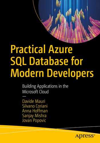
Azure SQL enables you to parse JSON text and extract information from JSON documents, store JSON text in the tables like any other type, and produce JSON text based on a set of rows.
Azure SQL enables you to work with JSON text that you are storing in tables or sending from your application by applying built-in functions JSON_VALUE, JSON_QUERY, ISJSON, and JSON_MODIFY. These functions enable you to parse JSON from text and extract and modify information in JSON documents.
If you want to transform your semi-structured data represented in JSON format and load JSON documents into tables, you can use OPENJSON function . The OPENJSON function takes an array of objects in JSON format and splits them into a set of rows. You can use this Table-Valued Function to transform JSON into tables and load data in a relational format.
Azure SQL also enables you to format the results of the SQL queries into JSON format. There is a FOR JSON clause that can specify that the results of the query should be returned in JSON format instead of a set of rows.
And here’s a Full-Stack example of the ToDoMVC sample app, implemented using NodeJS, Azure Functions, and Azure SQL, using JSON as transport format:
Formatting query results as JSON document
Modern applications are commonly implemented as distributed services that are exchanging data via HTTP endpoints. In most of the cases, the data is exchanged in JSON format.
Back-end developers spend a lot of their time getting the data from the database and serializing the results as JSON text that will be returned to the caller (e.g., front-end code). You might find a large amount of back-end code in a REST API that is just a wrapper around SQL queries. Some model classes are used just to temporarily load a set of rows returned as a result of SQL queries into memory and then immediately serialize these memory objects as JSON text that will be returned to the caller. This is known as the DTO (Data Transfer Object) pattern where model classes just transfer data between the application layers. Many DTO-like model classes are not even used by back-end code and represent just a template that data access frameworks will use to load data and serialize it as JSON results. This might affect performance and especially memory consumption because data returned by a query is copied into model memory objects and then copied again into JSON text that will be returned as result. Besides resource consumption, this approach might increase the latency in your services, not to mention the fact that such code is just a very low added-value plumbing code. Every transformation is blocking, and the results returned by the query must be fully loaded into a collection of memory objects and then some serializer (like JSON.Net in .Net languages) serializes the entire collection as JSON text.
Azure SQL enables you to extremely simplify this process. FOR JSON query clause enables you to specify that the query results should be returned as JSON string and not as collection of rows. This way, you can directly stream the results of your query to the client instead of building the layers and wrapper that just pass parameters from client to the query and transform results as JSON results.
This action method uses .NET, the micro-ORM Dapper and the Dapper.Stream extension that enables you to execute a SQL query on a connection to Azure SQL. The query has FOR JSON clause that instructs Azure SQL to return results in JSON format instead of tabular format. QueryInto method – from the Dapper.Stream extension – will stream the JSON result into the body of the HTTP response. This way, you need two C# lines of code to transform your query into a JSON web service. FOR JSON clause enables you to easily finish the journey from any SQL query to a fully functional REST API with a couple of lines of code.
Storing JSON documents
In some cases, you will have data structures that have high variety, and these structures could not be effectively represented as normalized schema. In this case, you might follow the NoSQL approach and serialize complex structures as JSON text.
This way, you can store semi-structured data or data with volatile structure without creating a custom subset of tables for every new variation. In this scenario, log messages are write once and read many times, so we don’t need to worry about efficient updates of semi-structured values in JSON log columns.
If you decide to store data in a table, you need to understand how to parse the values from a JSON column and use them in queries, speed up queries using indexes, and ensure that JSON content is valid.
Querying JSON data
JSON_VALUE(json, path_to_value) function will return a scalar value from JSON document on the specified path.
JSON_QUERY(json, path_to_object) function will return a complex object or array from JSON document on the specified path.
JSON_MODIFY(json, path_to_object, json_object) will take the JSON document provided as the first argument and locate value or object on the path specified with the second parameter, and instead of this value, it will inject the value provided as third parameter. The first argument will not be modified, and the modified JSON text will be returned. If you provide NULL value as a third parameter, the value on the path will be deleted.
ISJSON(json_string) returns value 1 if the string provided as argument is properly formatted JSON and 0 otherwise.
Using these simple functions, you can parse any JSON text in columns, parameters, or variables and extract the values in any query clause. The path in these functions represents the location of a value within the JSON document. The syntax used in paths is easy to understand because it is similar to most of the modern object-oriented languages that reference the fields within the object (e.g., $.info[3].name.firstName).
Scalar values from the severity column are directly referenced, and scalar values from the JSON column are extracted using JSON_VALUE function. In this query, you can notice the true advantage of multi-model capabilities of Azure SQL. You are using one SQL language with few additional functions to process semi-structured data mixed with the scalar relational columns. If you are familiar with standard SQL language, learning JSON extension will be an easy task.
JSON paths
$ represents the current JSON document that is provided as a first argument of JSON function.
Field references start with a dot and reference the sub-property within the context. As an example, $.info.name.firstName will find an “info” property and then find name property within that object and then firstName object within name.
Array references that can be applied on arrays and reference elements by index. As an example, $.children[2].name will find a “children” array, take the element with index 2, and then find name property within that object. Indexes in the array references are zero-based.
With this syntax of JSON paths, you can reference any property within the JSON document using the same style that is used in object-oriented languages.
Collation awareness
- 1.
cote
- 2.
côte
- 3.
coté
- 4.
côté
Collation awareness is one important feature especially for international applications. The fact that JSON functions can leverage this feature makes it a powerful addition to multi-model capabilities of Azure SQL.
Ensuring data integrity in JSON documents
This way, you have full control over the storage process, and you choose when JSON data should be validated. In this example, a simple rule is used to make sure that values inserted in the log column are valid JSON documents. You can create custom rules that extract the values from a JSON document using JSON_VALUE function and compare the returned value in a separate CHECK CONSTRAINT.
Indexing JSON values
Clustered Columnstore indexes compress JSON documents and enable high-performance analytics on JSON values.
B-Tree indexes enable you to quickly find the rows with some value in the JSON column.
Clustered Columnstore indexes on top of tables with JSON documents are a good choice if you need to do analytics on JSON documents. Columnstore indexes will apply so-called batch mode processing where they will leverage vector processing and SIMD instructions that can boost performance of your analytic queries over JSON data.
The computed column $severity is just a named expression that exposes value from JSON content stored in column log. It doesn’t use additional space unless you want to explicitly pre-compute the extracted value by adding a PERSISTED keyword. Whenever you filter or sort rows using the JSON_VALUE(log, '$.severity') expression, Azure SQL will know that there is an index on the matching and use it to speed up your query.
Importing JSON documents
The first argument of OPENJSON function is a text containing the JSON array that should be parsed. This function expects to get an array of JSON objects where every object will be converted into a new row in the result. If the array that should be converted is placed somewhere within the document, you can provide a second parameter that represents a JSON path where OPENJSON function should find the array of objects that should be transformed to the resultset. Every object in the referenced array will become one object in the resultset that will be returned.
Name of the output column. If an optional JSON path is not provided, this name is also the key of the JSON property that should be returned as a result value in this column.
SQL type of the output column. OPENJSON will use the semantic of CONVERT T-SQL function to convert the textual value in parsed JSON text to SQL value.
Optional JSON path that will be used to reference the property in the JSON object that contains the value that should be returned. If this path is not specified, the name of the column will be used to reference the property. As an example, if the column name is severity and the JSON path is not specified, then OPENJSON will try to find a value on the $.severity path.
Optional AS JSON clause. By default, OPENJSON will use JSON_VALUE function to get the value from the object that is currently converted. Therefore, it cannot return sub-objects or sub-arrays. If there is a JSON object or array on that path, it will not be returned unless you specify the AS JSON clause.
The result of the OPENJSON function will be a resultset that can be inserted into the table.
Graph structures
Social networks where you have people connected with relationships like friends, family, partners, or co-workers
Transportation maps where you have towns and places connected with roads, rivers, and flight lines
Bill-Of-Materials solutions where you have parts connected to other parts that are themselves connected to other parts and so on
The graph structures might be represented as tables and foreign keys relationships in some scenarios. The key reason why you would choose graph model instead of relational model is when you are working on a project where relationships are dominant and there are a small number of entities connected to each other in many different, direct, and indirect ways. In fact, the key difference in that domain is the transitive nature of the relationship. The term transitive is hereby used for its mathematical meaning: if a is connected to b and if b is connected to c, then a is connected to c. In these cases, you would not be interested only in a single-hop relationship (like fetching order lines for an order via foreign key relationship), but in all the hops needed to move from one node to another. To do that efficiently, you would like to leverage graph-specific semantics for query processing. Examples might be abilities to find the transitive closure (is a connected to z?), to find a shortest path between two objects or recursively traverse across all relationships starting with a specified object.
In Azure SQL, nodes and edges are represented using special tables. You may be wondering why using relational tables has been the chosen implementation to represent graph elements and if that is a good idea at all.
First, it is very common to have some information tied to nodes and edges, and tables are a perfect structure to hold that information. A second benefit of using tables is that the Azure SQL query optimizer can be leveraged to improve overall query performance. The third benefit of this choice is that, as they are just tables, columnstore and indexes can be used to improve performance even further.
Airport is a node of the graph, but it behaves as a regular table. We can add any column, index, or constraint to describe information in this node. This is another example of how Azure SQL multi-model capabilities enable you to combine advanced battle-tested database features in the new scenarios. Node table has a hidden column that represents a unique identifier of the node that would be explained later.
This constraint specifies that you cannot use Flightline edge to connect nodes other than Airport. This constraint also defines what would happen with the edge if the node is deleted.
Loading graph data
The Flightlines CSV file contains information about source and destination airport and the name of the flight line between them. We need to join this data with Airports by Name column and get the $NODE_ID values that should be imported.
Querying graph data
This query will return all destinations from Belgrade to all other towns. MATCH clause defines that a path from source airport (src) to destination airport (dest) should be established via flight line table (line).
The SHORTEST_PATH clause within the MATCH clause will find the shortest path between starting and end location that are not directly connected. Aggregate STRING_AGG will concatenate all airport names on the path and display them with arrow -> separator. COUNT and LAST_VALUE will show the number of stops on itinerary and ending flight and town on the shortest route. Once the shortest path exploration is finished, we need to select destination towns in the final query.
Graph processing capabilities in Azure SQL enable you to reduce complexity of your models and queries that should analyze different paths and relationships between tables.
Spatial data
Representing spatial objects (places, roads, country borders) is something that doesn't ideally fit into a structured relational model in normal form. Although you can represent a road or a border as a set of small straight lines where every line is stored in a separate row with the ends connected to the lines that continue the road, this is not an efficient representation.
The queries that you would run against spatial objects usually have conditions like “is this place within the shape” or “how far is the place from the road.” These are not the typical queries that you would describe using standard SQL language.
Specialized types that can be used to represent complex geometrical and geographical objects and shapes (Point, Line, Polygon). All shapes can be represented as geometry or geography models, which will be described more in detail soon.
Functionalities specialized for spatial querying such as finding the distance between two points (ST_DISTANCE), determining whether an area contains a specified point (ST_CONTAINS), and so on.
Specialized indexes that are optimized for spatial types of queries.
This set of capabilities enables you to create advanced queries that are specific for spatial domains.
Remember the airport and flight line model described in the previous section. Graph models that connect airports (nodes) using flight lines (edges) might be perfect to find the shortest route between two towns. However, imagine that you need to find all airlines that are crossing Nebraska or unnamed crossroads where two highways intersect. If there is no explicit relationship between highways and all crossroads or countries, it would be impossible to answer these questions.
GEOMETRY type represents data in a Euclidean (flat) coordinate system.
GEOGRAPHY type represents data in a round-earth coordinate system.
Geometry is perfect for representing relatively small objects like buildings or interiors; Geography is better suited to represent much bigger shapes, like river, city, or nation boundaries and in general anything that needs to work on close approximation of Earth surface to avoid errors.
Point used to represent 2D places like towns
LineString and CircularString that can represent open or closed lines like roads or borders
Polygon and CurvePolygon used to represent areas like countries
MultiPoint, MultiLine, and MultiPolygon representing a set of disconnected geographical objects that logically belong together (an archipelago with a set of islands might be represented with MultiPolygon)
In Azure SQL, once you have created a Geometry or Geography column in a table, you can use any of these types to build the shape you need. You can even use more than one at the same time, using Collections or “Multi” types.
Querying spatial data
STIntersects method determines if two shapes intersect at some place. This method returns 1 if a geography instance intersects another geography instance and 0 otherwise.
The spatial queries are enabling you to easily perform specific analysis to resolve problems where you would need to spend a lot of time dealing with the specific mathematical transformations, without having you to write them yourself or to use another more specialized solution to perform the calculation, so that you don’t have to move the data around, thus making your solution much more efficient.
Spatial indexes
In theory, STIntersects method might be implemented as a self-contained function with complex mathematical calculations that are trying to determine relationships between the figures. However, due to complexity of calculations, running that kind of function on many objects would be both time- and CPU-consuming. For efficient processing, Azure SQL uses a special type of Spatial indexes.
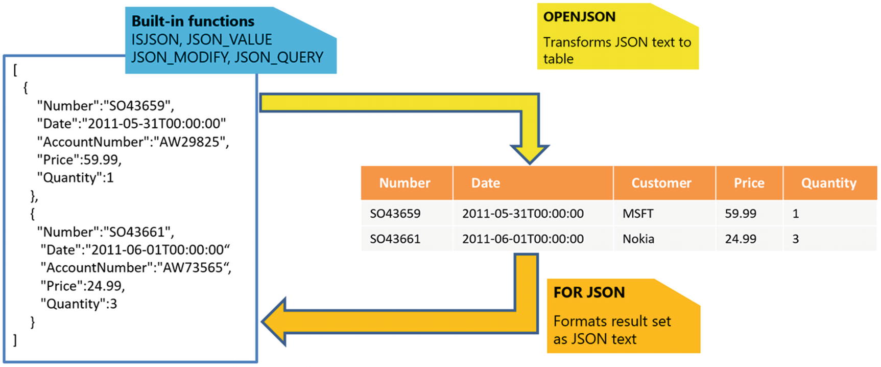
Indexing spatial objects in 4x4 grid
Azure SQL creates a grid, and for every spatial object that should be indexed, it records whether it fully or partially overlaps or doesn't overlap at all with the cells in the grid. This process is known as tessellation . With this technique, a STOverlaps method that needs to determine if two objects overlap will not immediately need to apply complex mathematical calculations to determine if there is some intersection between the objects. If an index is available, it will first use the index to check if there is at least one cell in the grid that belongs to both spatial objects or if the cell that belongs to one object also partially overlaps with another object. If this is true, then they overlap, and this is the faster way to determine if there is some interception. If there are no cells that at least partially overlap with both objects, then these objects do not overlap. If there are some cells that partially overlap with both objects, these objects might or might not overlap. Only in this case will Azure SQL apply complex spatial calculation, but not on the entire area of objects, just on smaller cells where they might potentially overlap. Although this might be CPU-consuming operation, it is performed on a small cell and probably the small part of objects that is within this cell. Therefore, this action would be few orders of magnitude faster than the naïve approach that would compare all parts of the objects.
Besides the spatial column that should be indexed, you can specify the characteristics of the grid that will be created to index the spatial values such as area that should be covered or density of tessellation grid used for indexing. More granular indexes will be bigger and need more time to scan all grid cells and determine whether the parts of the routes overlap with every cell. However, the bigger density of grids makes the worst-case scenario stage, where objects partially overlap much faster because smaller parts of the objects are processed using the complex math rules. This right size and parameters of the indexes depend on your data, and you might need to experiment and rebuild the index with different parameters to find what is the best fit for your data.
If you are unsure at the beginning, you can avoid the bounding box specification, and Azure SQL will try to guess the best bounding box and tessellation for you. Of course, the automatically defined values may not be the perfect ones in your scenario, so it is good to know that you can manually specify them if needed.
Geometry vs. Geography
Geometry data types are used to represent planar mathematical shapes in classic 2D coordinate system.
Geography data types are used to represent spherical objects and shapes projected into 2D plane.
The difference between geometry and geography types is one of the most important things that you need to understand to develop spatial applications.
Geography types are used to represent the objects placed in a classic 2D coordinate system, and you can imagine them as the objects that you could draw on the plain piece of paper. Distances and sizes of the objects are measured the same way you would measure distance of the objects drawn on a paper or a board. If you take a map and want to find the shortest flight trajectory between Belgrade, Serbia, Europe, and Seattle, Washington, US, you would probably use the straight horizontal line going via France and the US east coast. This is geometrically the shortest line between them. However, due to the rounded shape of the earth, the shortest trajectory (called geodesic) is going via Iceland, Greenland, and Canada. Geography data model is considering Earth’s actual shape and is able to find the real-world shortest distance and path.
Mapping the Earth surface to a 2D plane is the most difficult spatial problem. Famous mathematician Carl Gauss proved in his Theorema Egregium (Latin for "Remarkable Theorem") that spherical surfaces cannot be mapped to 2D planes without distortion. You might notice on some maps that the territories closer to the poles such as Greenland, Antarctica, north of Canada, and Russia might look stretched or sometime bigger than actual. This happens due to the fact that dense coordinates closer to poles must be “stretched” to project them in 2D coordinates. To make things even harder, the Earth surface is not spherical nor even ellipsoid. Irregular shape of Earth and proximity to poles force people to use different strategies of mapping to 2D plane. There are mapping rules that preserve correct distance shortest paths, shape, and vice versa, but in every strategy, something will be distorted. That’s why every geography object has an associated Spatial Reference Identifier (SRID) that describes what spatial transformation strategy is used to translate the object from the earth globe into the 2D plane. SRID describes what coordinates are used (latitude/longitude, easting/northing), unit of measure, where is coordinate root, and so on. Azure SQL will derive information from SRID to compare positions of the objects.
Some countries need to use multiple SRID in their territory, especially if their north and south borders are far like in Chile. In these scenarios, you would need to align SRID before comparing positions of the geography objects. Specifying different SRID would result in the different positions or shapes. Measuring the differences between spatial objects with coordinates determined using different SRID would lead to wrong results. Therefore, in Azure SQL spatial operations cannot be performed between spatial objects with different SRIDs.
WGS84 is the most commonly used standard and is the one also used on the GPS system in our phone or car. If you are unsure of which SRID to use, very good chances are that WGS84 will work perfectly for you.
The good news for you is that all these complex transformations are built in into Azure SQL. The only thing you need to do is to leverage functionalities and learn the basic principles that will help you to understand how to use Spatial features.
XML data
XML data type is the older brother of JSON. This feature was introduced in SQL Server Database engine between 2000 and 2005, while XML was the mainstream format for data exchange between different applications.
OPENXML table value function that can parse an XML document
FOR XML clause that can format results of the query as XML document
XML type with methods for processing values in XML documents
If you have understood the OPENJSON function and FOR JSON clause explained in the section about JSON support, then you probably understand the purpose of OPENXML function and FOR XML clause. The difference between these XML functionalities and matching JSON functionalities are trivial, so they will not be explained in more detail.
The key difference between JSON and XML support in Azure SQL is native XML type. Unlike JSON support where JSON text is stored in native NVARCHAR type, XML has a dedicated SQL type. XML is standardized type in many languages (e.g., System.Xml.Document in .NET framework), so it makes sense to have parity in SQL type. The key difference is that in JSON cases you are using string-like functions to parse JSON, while XML content is represented as an object where you can use various methods to extract data.
Querying XML data
value(path, type) that returns a node or attribute from XML object and automatically converts it into a SQL type. You need to specify a standard XPath expression that targets a single value in the XML document.
query(path) – This method returns an object from the XML document on a specified XPath expression.
nodes(path) is very similar to OPENXML/OPENJSON functions, and it is used to transform an array of XML elements on the specified path to a set of rows that can be used in a FROM clause.
exists(path) is a method that checks if there’s an existing element on the specified path.
modify(path, type) method enables you to insert, delete, or replace values of some nodes in XML document.
The first query uses the value member function of @x variable to extract the values of family identifier and name of the family member with id 81 and the name of the member with identifier value equal to the variable @i.
The second query takes all /family/row nodes from XML document as a rowset under the condition that the id attribute of each row is less than 50 and greater than 5. Every node that satisfies this condition is returned as column named xrow. Method value() is used to extract the value that will be compared with 50 with SQL operator, while exist() method is used to directly push down predicate to XML variable. Finally, the methods value() and query() are used to get the name, identifier, and XML content from each returned row.
Another interesting feature is the ability to bind the values of SQL variables or columns in the XPath expressions. In the preceding example, you could see that the third expression in the first SELECT clause uses SQL variable @i from the outer script. This might be a flexible way to specify how to find the data.
Although XML functionalities in Azure SQL are not core scenarios that you will frequently use, given that XML is not a mainstream format anymore, you can still use them to resolve various problems that require querying and transforming XML data.
XPath and XQuery languages
XPath (XML Path Language) is a query language for selecting nodes from an XML document.
XQuery (XML Query) is a query and functional programming language that queries and transforms collections of XML data.
Hierarchical expressions – Use XPath to specify the path from the root of XML document to desired element within the document. As an example, XPath /Family/row/name is used to reference the elements <name> that are placed under the <row> element, which is placed under the <Family> element that is the root of XML document. There can be multiple elements that match the same XPath expression, so you should use indexing operator [] to specify the elements that match expression should be referenced.
Node and attribute references – XPath enables you to reference either node or their attributes. Any name that doesn't start with @ will be treated as a name of XML node, while the names starting with @ (e.g., @id in the preceding example) will be treated as an attribute.
Recursive expressions – In some cases, you don’t want to or cannot reference the entire path from the root, or you need to find elements that are positioned in the different locations of the document. Recursive operator // enables you to specify a “detached path” where XML functions will try to find any path that matches the expression right of the recursive operator. As an example, //row/name will find any <name> element within the <row> element that is placed anywhere in the XML document.
Predicates enable you to specify some condition that elements must meet to be matched with XPath expression. As an example, //row[@id=17]/name specifies that the XML methods should find any <name> element within the <row> element that has id attribute with value 17. The predicates are the easy way to filter out some nodes that don’t satisfy some condition.
XPath can be a very powerful language that you can use to declaratively specify criteria for selecting the information from XML documents.
You can also use other XPath features like namespaces that enable you to define the scopes of names and match only the names within the same namespace; seven-direction axis that enables you to reference parents, siblings, and descendants; or build-in functions that can help you transform the results within the expressions.
The XML nodes() method emits three XML rows from the variable @x used in the previous example, and then the query method processes them using an XQuery expression. In the body of the XQuery expression, the current node is assigned to the variable $r, and the return statement creates a new XML node where id attribute and content of the name node are injected in template. As a result, this XQuery expression will return transformed XML shown below the query. As you can see, XQuery has a lot of power that can be used to implement complex processing of XML elements.
XML indexes
The primary XML index is a pre-computed structure that contains the shredded values and nodes from the XML column. Azure SQL uses the values from primary index instead of invoking expensive parsing of XML type with value(), nodes(), or query() methods. This is very similar to automatic index on JSON documents that Azure Cosmos DB uses.
A secondary XML index improves the performance of the queries that search or filter XML documents using exists() method or returns multiple values from XML document using value() method.
Selective XML indexes index only specified paths in XML column. This is very similar to multiple B-tree indexes on the predefined XML expressions.
Selective XML indexes are the recommended approach for indexing based on the learnings from the multiple XML scenarios in SQL Server. The SQL Server team found that automatic indexing of all possible fields leads to large size of XML indexes, and on the other side, most of the indexed paths are not used. Therefore, selective XML indexes became the best choice and trade-off between usability, performance, and size.
In selective indexes, you can choose the paths that should be included in the index and specify their types. The queries that use value() function on doc column with XPath queries as defined in the index specifications would be able to leverage the sxi_doc index, gaining a huge performance boost, even while the index is very small.
Key-value pairs
Azure SQL doesn’t have a specialized structure that holds key-value pairs. The reason is simple: key-value maps can be implemented using the simple two-column table.
This structure enables fast retrieval of the keys using hash indexes, which is optimal for elementary get/put operations. Memory-optimized tables have optimistic lock-free data access, and SCHEMA_ONLY durability ensures faster updates because data is not persisted to disk. In addition, if the values are formatted as JSON format, we can use native JSON functions to filter and process data right in the database, as you learned at the beginning of this chapter.
One of the scenarios for key-value structures in Azure SQL is centralized caching. There is a well-known case study in SQL Server 2016 that showed how the customer replaced a distributed cache mechanism that was able to achieve 150K requests/sec on 19 distributed SQL Server nodes, with a memory-optimized table in a single server that increased performance to 1.2 million requests/sec. The targeted scenario was implementation of ASP.NET Session cache. Azure SQL uses the same technology as SQL Server, and the same technology can be used for caching in Azure cloud.
In many real-world projects, caching using a specialized engine is usually the preferred choice, but that means that you need to master another technology, and you need to figure out how to best integrate it with your solution. Usually this effort is a good choice as caching solutions are much cheaper than a full-blown Azure SQL database, but if you are already using Azure SQL in the first place, knowing that you have this ability right in the database can provide you an additional option that you may want to evaluate to simplify the overall architecture.
How to handle unstructured text?
The most difficult to handle but not so uncommon case is unstructured textual data. In some cases, you will have textual data that cannot be nicely organized in JSON or XML format, but you would need to implement some searches on that text. One common example is HTML code that is placed in the database. Ideally, HTML should be the same as XML if it conforms to XHTML specification, but in many cases, HTML might have some variation that breaks strict XML structure.
LIKE predicate uses the percent sign (%) to match zero or more of any character and the underscore (_) matches any one character. These special characters in the pattern expression on the right side of LIKE operator enable you to define various patterns such as text beginning or ending with some text sequence. LIKE operator is a very handy tool that is commonly used for text searches on small datasets. Azure SQL can optimize and use indexes even when using the LIKE operator, especially if you are using LIKE to search all text that starts with some prefix. In such cases, an index and the LIKE operator can provide very good performance. If you need instead to do a more complex search, for example, looking for specific words contained somewhere in your text, especially if you are working with bigger text sets, you might want to consider some text indexing solution described in the next section to improve performance even more.
Indexing unstructured text
An FTS index contains a set of text fragments (tokens) divided using a set of word breakers. The tokens in the FTS index have the keys of the origin rows where the text is found. FTS enables you to provide some simple description of text pattern and return the keys of the rows that match the criterion.
Querying unstructured text
CONTAINS and FREETEXT that check whether the values in some columns match the predicate defined in the text predicate
Table-value functions CONTAINSTABLE and FREETEXTTABLE that return identifiers of the rows where text matches some criterion
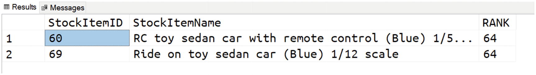
Table-value functions CONTAINSTABLE and FREETEXTTABLE match text based on exact or fuzzy match. One difference between these functions is that CONTAINSTABLE does more exact matching, while FREETEXTTABLE uses fuzzy matching using thesaurus, synonyms, and inflectional forms. If the word "children" is provided as a search criterion, FREETEXTTABLE will also match rows containing "child", but CONTAINSTABLE will not. In CONTAINSTABLE, you need to explicitly specify the expression FORMSOF(INFLECTIONAL,children) to instruct Azure SQL to include inflectional forms of this word.
Another difference is that CONTAINSTABLE enables you to specify operators like AND, OR, or NEAR to define how you want to search text. In the previous examples, you might see that we have provided set of words "blue car" to FREETEXTTABLE, and this function will return all rows that have any of these words like in most web search engines. In the CONTAINSTABLE example, we need to explicitly specify operators like AND, OR, or NEAR to specify what should be searched, for example, "blue AND car" or "blue OR car".
If there is some stock item containing the word 'cars', it will not be returned in the result because CONTAINS uses exact match using the word 'car'. However, if we use FREETEXT with 'children cars' search expression, this predicate will use inflectional forms of both words.
Full-text search is a very powerful tool that can help you to implement very complex searches with a simple expression.
How to leverage unstructured indexes on semi-structured data?
Full-text search is not limited only to unstructured text. You can use FTS indexes to improve performance of some JSON search queries where you need to filter documents that have key-value pairs defined by the client. After all, an FTS index is very similar to a Generalized Inverted Index (GIN) that is used in many databases exactly to index JSON data.
Let’s imagine that we need to implement functionality that searches a large set of JSON documents using arbitrary key-value combinations. Adding a B-Tree index on every possible key would be inefficient, and a CLUSTERED COLUMNSTORE index on JSON data is designed for analytical use cases and thus is not a good solution for filtering.
The NEAR operator in the CONTAINS predicate is a good choice for JSON scenarios where key of json property is near value. This kind of predicate will quickly find all text cells that have words "Color" and "Silver" close together, which is actually the case in JSON structure. In addition, CONTAINS clause enables us to specify complex predicates with AND, OR, and other relational predicates. However, FTS will not guarantee that "Color" is key and that "Silver" is value in the text, because it doesn’t understand the semantic of text parts in JSON structure. If you have some JSON document containing text "color silver", it will be returned by CONTAINS predicate, although this is not key-value pair.
CONTAINS will quickly filter out most of the entries that don’t satisfy the condition and might significantly reduce the number of candidate rows that might contain the needed data. Without this part, we would end up with full table scan and applying the JSON functions on every row.
JSON_VALUE will perform an exact check on the smaller candidate set returned by FTS. These predicates guarantee that correct results will be returned, and we are sure that we don’t need to apply them on every document.
This example again shows how Azure SQL features nicely fit together and enable you to implement various scenarios.
Multi-model in Azure SQL: why and when
Azure SQL is a modern multi-model database platform that enables you to use different data formats and combine them in order to design the best data model that will match the requirements of your domain. Depending on your scenario, you can represent relations as classic foreign key relationships or graph nodes/edges. Semi-structured data can be stored in JSON, Spatial, or XML columns.
You just learned how you can use all these features. It’s now time to discuss why and when.
One of the biggest advantages of Azure SQL is interoperability between core database features and multi-model capabilities. You can easily combine Columnstore with graphs or JSON data to get high-performance analytics capabilities on graph/JSON data, built-in language processing rules to customize application for any market, use all features that T-SQL language provides to create any query or powerful report, and integrate it with a variety of tools that understand T-SQL.
With Azure SQL, you are getting the core functionalities that other NoSQL databases provide, plus a lot of standard relational database functionalities that can be easily integrated with NoSQL features. This is the most important reason why you should choose the multi-model capabilities of Azure SQL.
So, should you choose Azure SQL with its multi-model capabilities or some specialized NoSQL Database engine that has more advanced features in these areas? That’s a very interesting – and not easy – question to answer.
Azure SQL is not a NoSQL database. If you have a classic NoSQL scenario that requires advanced graph or document support and you don’t expect to have to deal with other data that would otherwise be better stored into a table, then you should surely evaluate full-fledged graph or document databases such as Azure Cosmos DB, MongoDB, Neo4j, and so on. These database engines are fully oriented on NoSQL scenarios and have implemented richer and more advanced NoSQL features. They address a very specific area and they are extremely good at it.
The most important question that you need to ask yourself is what kind of additional NoSQL functionalities would your application need. Both Azure SQL and NoSQL database engines provide similar levels of fundamental graph and document processing functionalities (e.g., inserting, modifying, indexing, and searching). If you need more than these basic features, Azure SQL gives you an ability to leverage advanced querying using T-SQL, Columnstore technology for analytic, built-in machine learning capabilities with R/Python support, collations, replication mechanisms, and other functionalities that are proven as necessary in most of the real-world application. If you believe that these functionalities might be important for your application, then Azure SQL is the right choice for you.
If you want to know more
Multi-model capabilities of Azure SQL Database & SQL Managed Instance – https://docs.microsoft.com/azure/azure-sql/multi-model-features
Dapper.Stream – https://github.com/JocaPC/Dapper.Stream/
JSON Data in SQL Server – https://docs.microsoft.com/sql/relational-databases/json/json-data-sql-server
Getting started with JSON features in Azure SQL – https://docs.microsoft.com/azure/azure-sql/database/json-features
Graph processing with SQL Server and Azure SQL – https://docs.microsoft.com/sql/relational-databases/graphs/sql-graph-overview
Spatial Data – https://docs.microsoft.com/sql/relational-databases/spatial/spatial-data-sql-server
Spatial Indexes Overview – https://docs.microsoft.com/sql/relational-databases/spatial/spatial-indexes-overview
World Geodetic System (WGS84) – https://gisgeography.com/wgs84-world-geodetic-system/
Full-Text Search – https://docs.microsoft.com/sql/relational-databases/search/full-text-search